Oct 4, 2013 - James T. Curran received a B.E. in Electrical & Electronic ... of the European Microwave Signature Laboratory and leads the JRC ..... The host PC used was an Apple Mac-Mini connected to an array of hard-drives [21]. The IF ...
An Open-Loop Vector Receiver Architecture for GNSS-Based Scintillation Monitoring James T. Curran, Michele Bavaro & Joaquim Fortuny Institute for the Protection and Security of the Citizen, European Commission Joint Research Centre (JRC), Ispra (VA), Italy. Email: james.curran, michele.bavaro, joaquim.fortuny @ec.europa.eu.
Abstract: This paper explores the custom design of a scintillation-monitoring receiver. An open-loop vectorarchitecture is is proposed in which GNSS signals are processed in an entirely feed-forward manner. The benefits of this architecture are explored relative to commercial atmospheric monitoring receives, using datasets recorded at an equatorial site, exhibiting high ionospheric scintillation. The analysis focuses on the availability and quality of intensity and phase scintillation metrics, namely σφ and S4 . Result demonstrate the effectiveness of an open-loop architecture which can provide measurements comparable to those of a state-of-the-art commercial solution.
Biographies James T. Curran received a B.E. in Electrical & Electronic Engineering in 2006 and a Ph.D. in Telecommunications in 2010, from the Department of Electrical Engineering, University College Cork, Ireland. He worked as a senior research engineer with the PLAN Group in the University of Calgary from 2011 and is currently a grant-holder at the Joint Research Center (JRC) of the European Commission (EC), Italy. His main research interests are signal processing, information theory, cryptography and software defined radio for GNSS. Michele Bavaro received his master degree in Computer Science in 2003 from the University of Pisa. Shortly afterwards he started his work on Software Defined Radio technologies applied to navigation. First in Italy, then in The Netherlands and in the UK he worked on several projects being directly involved with the design, manufacture, integration, and test of RNSS equipment and supporting customers in the development of their applications. Today he is appointed as grant-holder at the EC JRC. Joaquim Fortuny-Guasch received the Engineering degree in telecommunications from the Technical University of Catalonia (UPC), Barcelona, Spain, in 1988, and the Dr.-Ing. degree in electrical engineering from the Universität Karlsruhe (TH), Karlsruhe, Germany, in 2001. Since 1993, he has been working for the Joint Research Centre (JRC) of the European Commission, Ispra, Italy, as senior scientific officer. He is the head of the European Microwave Signature Laboratory and leads the JRC research group on GNSS and wireless communications systems.
1
Introduction
Space-based radio signals are used extensively for atmospheric monitoring. As these signals propagate from their space-based transmitters to the earth, the atmosphere induces phase shifts, group delays, and amplitude variations. A receiver which processes these signals in an appropriate fashion can extract an estimate of these phase, delay and amplitude variations and can, in turn, infer some information about the atmosphere . Global Navigation Satellite System (GNSS) signals are widely used for this purpose, due both to their abundance, their global coverage, and the fact that they are transmitted at more than one frequency [1, 2]. The ionosphere and troposphere are monitored using these signals as they both induce propagation speed and direction changes to signals transmitted in the L-band. GNSS-based studies of the ionosphere are typically conducted using navigation receivers which track both the carrier and code phase either on a satellite-by-satellite basis, or collectively via a vector structure 1
[1]. Information relating to phase and amplitude scintillation is gathered from the receiver’s estimate of the carrier phase and the receiver correlators values, respectively. The quality of these parameters, however, is directly influenced by how well the receiver can track the GNSS signals. Under scintillation conditions these measurements are corrupted and degraded as the errors in the code and carrier tracking loops grow [3, 4]. Code-phase biases will manifest themselves as amplitude fades and carrier phase cycle-slips will appear as large, sudden phase fluctuations. Given such corrupted data it can be difficult to distinguish between receiver-induced artefacts and ionosphere anomalies. Moreover, if a receiver cannot acquire or track the signal, these measurements are simply not available [4]. In light of the limitations of navigation-receiver based monitoring, this paper explores the custom design of a Scintillation-Monitoring Receiver (SMR). The navigation capabilities of a traditional SMR are often redundant as such receivers are typically fixed at known coordinates. Indeed the entire acquisition and tracking process is avoidable. This fact is exploited in the receiver design wherein an open-loop architecture is adopted. Rather than tracking the range and range-rate to each satellite in view, this architecture leverages knowledge of the receivers position in time and space and satellite ephemeris to demodulate the received signals in an entirely open-loop manner. In an inversion of the traditional navigation receiver, which uses measurements of signal parameters to compute an estimate of position and time; this architecture uses knowledge of position and time to estimate local-replica signal parameters for demodulation purposes in a pure feed-forward fashion. Essentially an open-loop vector demodulation scheme, it can produce a series of baseband correlator values from which the deterministic phase process induced by satellite-to-user dynamics and receiver clock effects have been removed. What remains are a series of complex values modulated only by the amplitude and phase processes corresponding to the ionospheric activity. These can then be post-processed in a noncausal or batch mode to reconstruct the phase and amplitude processes and extract traditional metrics such as σφ or S4 , or even to explore new scintillation characterizations [5, 6]. It will be shown that this architecture can deliver a two distinct advantages over the traditional navigationreceiver approach. Firstly, as this is an open-loop architecture, it does not suffer from cycle-slipping or loss of lock. When deep amplitude fades occur, they do not affect the quality of the demodulation and, in contrast to traditional receivers, this architecture does not need time to re-acquire, re-stabilize or recover. Thus the receiver is capable of providing greater availability of higher quality correlator values, the raw measurements needed for ionosphere characterization, than a standard navigation receiver. Secondly, by using predictions of the systematic range and range-rate contributions to the received signal parameters, the baseband correlator values will be inherently free of systematic effects and receiver processing artefacts. Traditionally, researchers have relied on high-pass and low-pass filters for de-trending the receiver carrier phase and signal intensity estimates. However such de-trending cannot reject some receiver-based tracking errors such as cycle-slipping which can lead to contaminated measurements. The new architecture offers resilience to such effects. In particular it will facilitate the use of open-loop batch processing of correlator values for optimal phase reconstruction [7–9].
2
Signal Model & Scintillation Statistics
Typically the GNSS signal received at the antenna of a ground-based receiver is be modelled as an ensemble of signals from each of the satellites in view, plus a thermal noise interference. Modern GNSS receiver employ either: one or more heterodyne stages followed by sampling and digitization, or direct digital downconversion, to either a low or zero Intermediate Frequency (IF). In either case, the result is a sequence of digitized samples, rendered at a rate of 1/Ts , given by:
r [k] =
X
si (kTs ) + n (kTs )
i∈Sig
si (t) =
p
2Pi (t)di (t − τi (t)) ci (t − τi (t)) sin (ωi t + θi (t)) ,
(1)
where Sig is the set of satellite signals in view, si (t) denotes the ith signal received from the visible satellites and n (t) denotes the additive thermal noise. The various parameters in (1) represent the following signal properties: Pi is the total received signal power in watts; ωi is the nominal IF carrier frequency in units of rads−1 ; di (t) represents the bi-podal data signal, if present; ci (t) represents the combination of the secondary code, the primary spreading sequence and the sub-carrier; θi (t) is the total received phase process including propagation delays, satellite-to-user dynamics, atmospheric effects and satellite clock effects; the process τi (t) represents the total delay observed at the receiver, including propagation delay, satellite clock effects and atmospheric delays. 2
Ts TI
r (mTs )
å
yi [n]
ci (tˆi (mTS )) exp{- j (wˆ i mTS + qˆi (mTS ))}
qˆi (mTS ))
tˆi (mTS )
Figure 1: A block diagram of a Digital Matched Filter (DMF). The carrier phase term, θi (t) in (1) represents a number of distinct phase processes. It can be represented as the linear combination:
θi (t) =θ0 + θLOS (t) + θSV Clk. (t) + θRx Clk. (t) + θAtm. (t) ,
(2)
where θ0 represents some arbitrary initial phase, θLOS (t) represents the phase process induced by the lineof-sight geometry/dynamics between the satellite and the receiver, θSV Clk. (t) and θRx Clk. (t) respectively represent the phase processes induced by errors in the satellite and receiver clocks, and θAtm. (t) represents the phase process induced by the atmosphere through which the signal propagates. Similarly, the received power, Pi (t) in (1) can be represented by the product:
Pi (t) = PSV × LLOS (t) × LAtm. (t) × LRx (t) ,
(3)
where PSV represents a nominal transmitted power, LLOS (t) represents free-space loss across the lineof-sight range the satellite and the receiver, LAtm. (t) represents the effective power loss induced by the atmosphere through which the signal propagates, and LRx (t) represents the loss (or gain) induced by the receiver antenna, front-end and digitization process [10]. The terms θAtm. (t) and ×LAtm. (t) are of interest here. As GNSS signals are received at the earth at a very low nominal power, typically below the thermal noise floor, it is necessary to employ a DMF, introducing sufficient correlation-gain (of the order of 30 to 40 dB) to enable a receiver to acquire and track the signals. The DMF operation can be expressed as follows: T
1 Yi [n] = TI
(n+1) TIs −1
X
T k=n TIs
�
� ˆ r (kTs ) ci (kTs − τˆi (kTs )) e−j (ωi (kTs )+θi (kTs )) ,
(4)
where the variables τˆi and θˆi are the receivers estimate of the variables τi and θ and the term Yi [n] is known as the correlator value [10] and is computed across an interval TI , which typically ranges from one to one hundred milliseconds. A block diagram of this operation is presented in Figure 1. In a traditional GNSS receiver, one or more correlator values may be produced, with prescribed code and/or frequency offsets relative to the current estimates of τˆi (kTs ) and θˆi (kTs ), for example a standard Delay-Lock Loop (DLL) will require two extra correlator values, generated with ’early’ and ’late’ code replicas. In any case, the correlator values will be processed by a set of code and carrier tracking loops, or a central socalled vector tracking loop, to recursively estimate the next set of values of τˆi ((k + 1) Ts ) and θˆi ((k + 1) Ts ). Although both the code and carrier phases are representative of the range and range change between the satellite and the receiver, due to their significantly different periods, they are generally used in different applications. As GNSS signals have wavelengths in the range of 18 to 27 cm, carrier phase measurements and 3
can provide a particularly sensitive means of observing changes in the propagation delay. For the purposes of atmospheric scintillation monitoring, when only the temporal or spacial variations in the signal delay are of interest, the carrier phase is generally utilized. Traditionally the effects of ionospheric scintillation on the received signal amplitude and phase have been examined using statistics known as the amplitude and phase scintillation indices, respectively denoted S4 and σφ . Essentially, S4 is a measure of the variation of instantaneous received signal amplitude relative to the average received signal amplitude over a certain period of time [11] and σφ is a measure of the variations in received signal phase, relative to the nominal phase trajectory that would be observed under non-scintillation conditions. In both cases, the temporal variations are examined relative to a non-constant value which is not directly accessible to the receiver and so care must be taken when performing these measurements. In the case of S4 , this non-constant value is the nominal received signal power, and in the case of σφ it is the nominal phase trajectory. In general, receivers implement a so-called de-trending operation which endeavours to separate the deterministic, slowly-varying contributions to the amplitude and phase processes, Pi (t) and θi (t), that are induced by, for example, line-of-sight displacement, the receiver antenna, and the local oscillator; from the stochastic, more rapidly varying scintillation-related contributions. Historically, the spectral separation of the deterministic ‘trends’ and the random scintillation effects have been exploited, and receivers have employed high- and low-pass filters for this purpose [11, 12]. As carrier phase is regularly employed for navigation purposes, θˆ is readily available in many GNSS receivers, however a measure of the instantaneous received power is less common and, typically, must be estimated from the correlator values. The square magnitude of y offers a suitable approximation under high signal-to-noise ratio (SNR) conditions while for low SNR conditions the bias due to thermal noise might also be removed. As the power estimate is normalised by the S4 calculation, any estimate of the received power which satisfies Pˆ ≈ kP across the expected received power range, will suffice. Indeed, in the case that the receiver thermal noise floor is reasonably unvarying, a linear measure of C/N0 can be used, provided it has not been excessively smoothed or filtered [1, 12]. Typically this estimate of received power is termed the signal intensity and is denoted here by I . The S4 and σφ metrics are calculated from raw receiver measurements according to:
�. � � 2 2 hIiT I 2 T − hIiT
� 2 σφ = φ2 T − hφiT , S4 =
(5) (6)
where the notation h·iT denotes the temporal average over some fixed period, T . Various values of T have been employed in the literature with the more widely accepted values being 20 and 60 seconds [11, 12]. At this point it is worth noting that the traditional techniques, as described above, require that the receiver be capable of coherently tracking the received signal carrier. In the proposed open-loop architecture that will be described next, phase-coherence is not assured and, therefore, the techniques used to generate the measurements S4 and σφ must be modified accordingly. The traditional techniques, and a discussion on various factors that influence their performance, along with details of the modified technique, will be discussed in Section 3.3.
3
Scintillation Monitoring Receiver Architecture
This section describes an open-loop receiver architecture that can be applied to the challenge of ionospheric scintillation monitoring. The receiver, a simplified block diagram of which is presented in Figure 2, comprises of three distinct sub-systems: a data-acquisition section, DAQ, an open-loop demodulation unit, OLD, and a unit which implements the atmosphere monitoring algorithms, AMA.
3.1
Data Acquisition
The DAQ module performs the analogue Radio Frequency (RF) to digital IF conversion. It comprises of an antenna, a reference clock and a digitizing front-end, which performs filtering, down-conversion, sampling and digitization of one or more GNSS bands. The IF samples can then be either streamed directly to the OLD module, or stored for post-processing. Each sample captured by the digitizer is associated with a receivetime as reported by the reference clock and, ideally, will coincide with the true GNSS time. This time-tag is used by the OLD module in the generation of local replica signals for demodulation.
4
r DAQ
yi
OLD
AMA
TOW S.V.
Rec.
Atm.
Figure 2: Block diagram of the system architecture. The system consists of three main components: DAQ which performs the task of IF data acquisition and time-tagging, OLD which performs the demodulation of the received signal to produce the correlator values, ad AMA which generates the atmospheric measurements. While, in principle, any digitizing front-end can effect a suitable DAQ module, two features are critical and must be considered. Firstly, the behaviour of the Automatic Gain Control (AGC) has a direct influence on the observed variations in the signal power at IF which, as can be seen by inspection of (3) and (4), can corrupt measurements of S4 . To avoid measurement corruption, the AGC must be configured to either: maintain a constant gain over the observation period; exhibit a sufficiently low slew-rate as to allow its effect to be removed via de-trending; or the AGC gain may be recorded to facilitate post-correlation normalization. Secondly, the quality of the reference clock plays a significant role in the behaviour of the DAQ, both in terms of phase and amplitude scintillation measurements. Examining (2) and (4), it can be seen that the reference clock phase noise will contribute to the observed phase scintillation measurement. Also, as will be discussed further in Section 3.2, errors in the reference clock will manifest themselves in misalignments between the received spreading code sequence and local replica, ci (kTs − τˆi (kTs )), in (4), thereby inducing variations in the magnitude of Yi [n]. To minimize these effects, the reference clock should exhibit good shortand long-term stability. It should exhibit a very low phase noise and the bias and drift terms should either be negligible or accurately modelled. The constraint of having a sufficiently stable phase reference to perform accurate phase scintillation measurements is, essentially, unavoidable and has been addressed by using a reference oscillator designed specifically do exhibit low phase noise. Unlike the problem of stochastic phase noise, the long-term drift and drift rate of the oscillator does not pose as significant a challenge. Although a clock that is perfectly aligned with the GNSS time is preferable, long-term drift can be readily measured in advance, and the clock offset propagated appropriately through the measurement period. By observing the received GNSS signals for a short time both before and after the measurement period, the clock bias and drift can be very well modelled throughout the measurement itself.
3.2
Open-Loop Demodulation
The signal demodulator is the heart of the receiver architecture, processing the time-tagged IF samples captured by the DAQ to produce baseband correlator values. Unlike a traditional GNSS receiver, the demodulator does not rely on feedback mechanisms to produce estimates of the current signal parameters such as carrier and code phase. Rather, it relies on prior knowledge of the satellite and user trajectories, time, and some broadcast propagation models. As such, it performs the demodulation in an open-loop manner. In this study, the monitoring receiver has been installed at well-survey, fixed location, such that the position of the antenna phase centre is known to centimetre accuracy. Knowledge of the satellite position can be derived either through broadcast or precise ephemerides. When post-processing IF data that has been collected and stored some time previously, for example the previous day, collated broadcast ephemerides can be sourced from sources such as the International GNSS Service [13]. Alternatively, for live processing ephemerides can be sourced for nearby reference stations. One particular benefit of this scheme is that signals can be readily tracked even if they are well below the data-demodulation threshold. Provided that one station, somewhere on earth, has successfully extracted an valid ephemeris record, the received satellite signal can be processed. As ionospheric activity can be quite specially uncorrelated, one station may enjoy perfect reception conditions while another, some hundreds of kilometres away may observe severe scintillation. The demodulation process operates as follows. Each sample stream originating from the DAQ has an associated centre frequency and bandwidth and each sample within that stream has an associated time-tag.
5
5
x 10
PRN 5 PRN 15 PRN 18 PRN 21 PRN 24 PRN 26 PRN 29 PRN 30
Received Signal Strength
6 5 4
1.5
In-phase and Quadrature Correlator Values
7
3 2 1
0 −400
−300
−200
−100 0 100 Receiver Clock Bias (m)
200
300
x 10
1
0.5
0
-0.5
-1
-1.5 0
400
7
2
4
6
8
10
Time (s)
(a) Received signal power versus time-tag error for all visible GPS L1 CA signals.
(b) Complex correlator values of an open-loop GPS L1 CA demodulated signal.
Figure 3: Open-loop demodulation of a received signal. For each of the satellite signals which lie within the sample stream bandwidth, a visibility check is computed using the corresponding ephemeris record and the IF sample time-tag. The visibility check coarsely evaluates evaluates the elevation from the known receiver position to the satellite position, computed at the current receiver time, and compares it to an elevation mask. For each satellite signal that is deemed visible, the effective transmit-time of the signal is calculated, via recursion, incorporating known receiver biases. A sample of the local replica signal is then computed to correspond to this transmit time, including carrier, subcarrier and primary (and secondary) code, and used to demodulate the received sample. As the effective transmit time is computed directly, the demodulated signal can be accumulated (or integrated) and dumped at boundaries of the transmit time, in this case at millisecond epochs in the transmit time. An example of the average complex envelope of the correlator values, versus receiver clock bias is shown in Figure 3a for a selection of GPS L1 C/A signals. As can be seen, the envelope exhibits the classical cross-correlation function observed during a traditional acquisition process. Evident also is the fact that the demodulation process does not perfectly align the local replica signals with their received counterparts. This is due, primarily, to the fact that the atmospheric errors have not been modelled in the demodulation process. Despite these biases, the ‘aligned’ or ‘prompt’ correlator still captures the majority of the received signal power and is, therefore, sufficiently aligned for the purposes of scintillation monitoring. The time-series of this prompt correlator is shown in Figure 3b wherein the residual errors after the open-loop demodulation can be seen as a rotation of the complex correlator values over time.
3.3
Atmospheric Monitoring Algorithms
This section of the receiver processes the complex correlator values, Y [n], generated in the demodulation stage, to generate atmospheric measurements, in particular this work examines the generation of ionospheric scintillation indices. Widely accepted parameters for scintillation characterisation are S4 for amplitude and σφ for carrier phase. Generally, calculation of S4 requires the calculation of an intermediate parameter, termed signal-intensity and denoted I , from the correlator values, Y [n]. In many cases this is often implemented via further intermediate variables, see, for example, [14, 15]. Alternatively, other implementations calculate this directly from the correlator values, [5, 6, 11, 12]. The particular implementation chosen in this work is depicted in Figure 4a. Specifically, an instantaneous measure of the signal power, Pˆ is computed as the square magnitude of the complex correlator values, minus an estimate of the thermal noise contribution:
Pˆ = |Yi |2 − 2σ 2
(7)
This value is then de-trended, via a normalisation operation, whereby the power estimate is divided by a low-pass version of itself. A 6th order Butterworth low-pass filter with 0.1 Hz bandwidth is generally employed, which, for numerical stability reasons, is implemented as a cascaded series of 2nd order filters. The signal intensity estimate, I , is calculated as:
I=
Pˆ hLPF ∗ Pˆ 6
,
(8)
yi
yi |·|
2
+| · |
2
+ y i
Pˆ
2ˆn2
2ˆn2
✓ˆ
Pˆ | · |2
+
⇥
÷
2ˆn2
LPF
LPF
(a) Block diagram of S4 calculation. ⌦ 2↵ +
LPF
+
LPF
ˆ
⌦
↵ 2
⌦
2
T M-FLT
↵
M-FLT
T
2
h iT⌦
M-FLT
⌦
2
↵
⌦
T
S4
2
↵
2
2
h iT ↵ 2
S S44
2
2
h iT
T
(b) Block diagram of σφ calculation.
ˆ
ˆ
hIiT
✓ˆ
LPF
↵
hIiT
2
LPF
+
✓ˆ
⌦ ↵⌦
2 2 ⌦I ⇥2 ↵ II 2 T I22 ThIihIi T T I ÷ T hIiT2hIi2T
⇥ Pˆ I÷
2 2
2
T
h iT
2
2
T
2
h iT
h iT
2
(c) Block diagram of σφ calculation.
Figure 4: Calculation of S4 and σφ from receiver measurements. where hLPF is the impulse response of the low-pass filter, and ∗ denotes convolution. This value is then processed according to (5) to produce the S4 measurements. The method of σφ calculation implemented in the receiver involves three steps, as follows [11, 12]. Firstly the phase of the received GNSS signal is reconstructed and sampled at a fixed sample rate, to produce the equivalent process θ [n] = θ (nTI ). Secondly, it is de-trended using a 6th order Butterworth high-pass filter with 0.1 Hz bandwidth. Finally, the variance of the de-trended phase process is calculated over fixed-length non-overlapping blocks of period T seconds. This process is depicted in Figure 4b, wherein the high-pass filter is implemented as the difference between the signal and low-pass component. A standard GNSS receiver typically derives carrier phase observations via a closed loop phase-tracking algorithm. Such as a Phase-Lock Loop (PLL) which will produce the entire phase trajectory, including the Doppler-induced phase trend, local oscillator effects and the ionospheric contribution. In contrast, in the approach described here, the received signals are demodulated to baseband, removing virtually all of the deterministic phase trend. This phase process is dominated by the ionospheric contribution plus some residual phase trends induced by factors such as, for example, errors in the satellite ephemeris. There are many benefits of this approach over closed loop tracking architectures. The availability of the correlator values is isolated completely from the receivers ability to track the signal. Indeed, received C/N0 or signal dynamics do not affect the receivers ability to produce Y [n]. As such, the time-series of complex correlator values can be simply post-processed to reconstruct the phase trajectory, allowing forward, forwardbackward, or batch processing, facilitating robust phase reconstruction and consistency checking. Specifically, the phase process is reconstructed as follows: the current correlator values are de-rotated by the previous phase estimate, the residual phase is estimated by a phase discriminator, and the value of the current phase is then computed as sum of the previous phase and the current residual phase. This process can be represented by:
Y 0 [n] = Y [n] e−iθ[n−1] ( atan2(d [n] < {Y ‘ [n]} , = {Y ‘ [n]}) ∆ [n] = ={Y ‘[n]} atan(