Hindawi Publishing Corporation Mathematical Problems in Engineering Volume 2016, Article ID 7126080, 10 pages http://dx.doi.org/10.1155/2016/7126080
Research Article An Operational Matrix of Fractional Differentiation of the Second Kind of Chebyshev Polynomial for Solving Multiterm Variable Order Fractional Differential Equation Jianping Liu, Xia Li, and Limeng Wu Hebei Normal University of Science and Technology, Qinhuangdao, Hebei 066004, China Correspondence should be addressed to Jianping Liu;
[email protected] Received 30 March 2016; Revised 29 April 2016; Accepted 4 May 2016 Academic Editor: Jos`e A. Tenereiro Machado Copyright © 2016 Jianping Liu et al. This is an open access article distributed under the Creative Commons Attribution License, which permits unrestricted use, distribution, and reproduction in any medium, provided the original work is properly cited. The multiterm fractional differential equation has a wide application in engineering problems. Therefore, we propose a method to solve multiterm variable order fractional differential equation based on the second kind of Chebyshev Polynomial. The main idea of this method is that we derive a kind of operational matrix of variable order fractional derivative for the second kind of Chebyshev Polynomial. With the operational matrices, the equation is transformed into the products of several dependent matrices, which can also be viewed as an algebraic system by making use of the collocation points. By solving the algebraic system, the numerical solution of original equation is acquired. Numerical examples show that only a small number of the second kinds of Chebyshev Polynomials are needed to obtain a satisfactory result, which demonstrates the validity of this method.
1. Introduction The concept of fractional order derivative goes back to the 17th century [1, 2]. It is only a few decades ago that it was realized that the arbitrary order derivative provides an excellent framework for modeling the real-world problems in a variety of disciplines from physics, chemistry, biology, and engineering, such as viscoelasticity and damping, diffusion and wave propagation, and chaos [3–6]. Orthogonal functions have received noticeable consideration for solving fractional differential equation (FDE). By using orthogonal functions, the FDE can be reduced to solve an algebraic system, and then original problems are simplified. Ahmadian et al. [7] proposed a computational method based on Jacobi Polynomials for solving fuzzy linear FDE on interval [0, 1]. Kazem et al. [8] constructed a general formulation for the fractional order Legendre functions. Y¨uzbas¸ı [9] gave the numerical solutions of fractional Riccati type differential equations by means of the Bernstein Polynomials. Kazem [10] constructed a general formulation for the Jacobi operational matrix for fractional integral equations.
Tau method and collocation method are widely used tools for the solution of FDE. Operational approach of the tau method was employed for solving fractional problems [11]. A numerical approach was provided for the FDE based on a spectral tau method [12]. An efficient method based on the shifted Chebyshev-tau idea was presented for solving the space fractional diffusion equations [13]. Tau method is very effective for constant coefficient nonlinear problems, but the method is not generally adopted for nonlinear FDE. In practice, since collocation method has the advantages of less computation and easy implementation, it is more widely applied for solving variable coefficient nonlinear problems. The collocation method was used for solving the nonlinear fractional integrodifferential equations [14]. The third kind of Chebyshev wavelets collocation method was introduced for solving the time fractional convection diffusion equations with variable coefficients [15]. From the literatures above, we conclude that many authors employed tau and collocation method for solving different kinds of FDE based on different kinds of orthogonal functions or their variants. However, for the aforementioned
2
Mathematical Problems in Engineering
FDE, the derivative order is a fixed constant, which does not change spatially and temporally; variable order multiterm FDE is not mentioned and solved. Therefore, our main motivation is to give a numerical technology for solving variable order linear and nonlinear multiterm FDE based on the second kind of Chebyshev Polynomial. With further development of science research, it is found that variable order fractional calculus can provide an effective mathematical framework for the complex dynamical problems. The modeling and application of variable order differential equation has been a front subject. In addition, the FDE is a special case of variable order ones, so it can also be solved by our proposed technology. Variable order derivative is proposed by Samko and Ross [16] in 1993, and then Lorenzo and Hartley [17, 18] studied variable order calculus in theory more deeply. Coimbra and Diaz [19, 20] used variable order derivative to research nonlinear dynamics and control problems of viscoelasticity oscillator. Pedro et al. [21] researched diffusive-convective effects on the oscillatory flow past a sphere by variable order modeling. The development of numerical algorithms to solve variable order FDE is necessary. Since the kernel of the variable order operators is very complex for having a variable exponent, it is difficult to gain the solution of variable order differential equation. Only a few authors studied numerical methods of variable order fractional differential equations. Coimbra [19] employed a consistent approximation with first-order accurate for solving variable order differential equations. Sun et al. [22] proposed a second-order Runge-Kutta method to numerically integrate the variable order differential equation. Lin et al. [23] studied the stability and the convergence of an explicit finitedifference approximation for the variable order fractional diffusion equation with a nonlinear source term. Chen et al. [24, 25] paid their attention to Bernstein Polynomials to solve variable order linear cable equation and variable order time fractional diffusion equation. A numerical method based on the Legendre Polynomials is presented for a class of variable order FDE [26]. Chen et al. [27] introduced the numerical solution for a class of nonlinear variable order FDE with Legendre wavelets. To the best of our knowledge, it is not seen that operational matrix of variable order derivative based on the second kind of Chebyshev Polynomial is used to solve multiterm variable order FDE. In addition, for most literatures, they solved variable order FDE defined on the interval [0, 1]. Accordingly, based on the second kind of Chebyshev Polynomial, we propose a new efficient technique for solving multiterm variable order FDE defined on the interval [0, 𝑅]. The multiterm variable order FDE is given as follows: 𝐷𝛼(𝑡) 𝑓 (𝑡) = 𝐹 (𝑡, 𝑓 (𝑡) , 𝐷𝛽1 (𝑡) 𝑓 (𝑡) , 𝐷𝛽2 (𝑡) 𝑓 (𝑡) , . . . , 𝐷𝛽𝑘 (𝑡) 𝑓 (𝑡)) , (1) 0 < 𝑡 < 𝑅,
where 𝐷𝛼(𝑡) 𝑓(𝑡) and 𝐷𝛽𝑖 (𝑡) 𝑓(𝑡) are fractional derivative in Caputo sense. When 𝛼(𝑡) and 𝛽𝑖 (𝑡), 𝑖 = 1, 2, . . . , 𝑘 are all constants, (1) becomes (2); namely, 𝐷𝛼 𝑓 (𝑡) = 𝐹 (𝑡, 𝑓 (𝑡) , 𝐷𝛽1 𝑓 (𝑡) , 𝐷𝛽2 𝑓 (𝑡) , . . . , 𝐷𝛽𝑘 𝑓 (𝑡)) ,
(2)
0 < 𝑡 < 𝑅. Thus, (2) is a special case of (1). Our proposed method can solve both (1) and (2). They often appear in oscillatory equations, such as vibration equation, fractional Van Der Pol equation, the Rayleigh equation with fractional damping, and fractional Riccati differential equation. The basic idea of this method is that we derive differential operational matrices based on the second kind of Chebyshev Polynomial. With the operational matrices, the equation is transformed into the products of several dependent matrices, which can also be viewed as an algebraic system by making use of the collocation points. By solving the algebraic system, the numerical solution is acquired. Since the second kinds of Chebyshev Polynomials are orthogonal to each other, the operational matrices based on Chebyshev Polynomials greatly reduce the size of computational work while accurately providing the series solution. From some numerical examples, we can see that our results are in good agreement with the analytical solution, which demonstrates the validity of this method. Therefore, it has the potential to utilize wider applicability. The paper is organized as follows. In Section 2, some necessary definitions and properties of the variable order fractional derivatives are introduced. The basic definitions of the second kind of Chebyshev Polynomial and function approximation are given in Sections 3 and 4, respectively. In Section 5, a kind of operational matrix of the second kind of Chebyshev Polynomial is derived, and then we applied the operational matrices to solve the equation as given at beginning. In Section 6, we present some numerical examples to demonstrate the efficiency of the method. We end the paper with a few concluding remarks in Section 7.
2. Basic Definition of Caputo Variable Order Fractional Derivatives Definition 1. Caputo variable fractional derivative with order 𝛼(𝑡) is defined by 𝐷𝛼(𝑡) 𝑢 (𝑡) =
𝑡 1 ∫ (𝑡 − 𝜏)−𝛼(𝑡) 𝑢 (𝜏) 𝑑𝜏 Γ (1 − 𝛼 (𝑡)) 0+
(𝑢 (0+) − 𝑢 (0−)) 𝑡−𝛼(𝑡) + . Γ (1 − 𝛼 (𝑡))
(3)
If we assume the starting time in a perfect situation, we can get Definition 2 as follows.
Mathematical Problems in Engineering
3 weight function is 𝜔(𝑡) = √𝑡𝑅 − 𝑡2 with 𝑡 ∈ [0, 𝑅]. They satisfy the following formulas:
Definition 2. Consider
𝐷𝛼(𝑡) 𝑢 (𝑡) =
𝑡 1 ∫ (𝑡 − 𝜏)−𝛼(𝑡) 𝑢 (𝜏) 𝑑𝜏 Γ (1 − 𝛼 (𝑡)) 0
̃ 0 (𝑡) = 1, 𝑈 (4)
(0 < 𝛼 (𝑡) < 1) .
By Definition 2, we can get the following formula [25]:
̃ 1 (𝑡) = 2 ( 2𝑡 − 1) = 4𝑡 − 2, 𝑈 𝑅 𝑅 ̃ 𝑛+1 (𝑡) = 2 ( 2𝑡 − 1) 𝑈 ̃ 𝑛 (𝑡) − 𝑈 ̃ 𝑛−1 (𝑡) , 𝑈 𝑅
(7) 𝑛 = 1, 2, 3, . . . ,
Γ (𝑛 + 1) { 𝑡𝑛−𝛼(𝑡) , { { Γ (𝑛 + 1 − 𝛼 (𝑡)) 𝛼(𝑡) 𝑛 𝐷𝑡 (𝑡 ) = { { { {0,
𝑚 ≠ 𝑛, { {0, 2 ̃ ̃ √ ∫ 𝑡𝑅 − 𝑡 𝑈𝑛 (𝑡) 𝑈𝑚 (𝑡) 𝑑𝑡 = { 𝜋 { 𝑅2 , 𝑚 = 𝑛. 0 {8 ̃ 𝑛 (𝑡) The shifted second kind of Chebyshev Polynomial 𝑈 can also be expressed as 𝑅
𝑛 = 1, 2, . . . , (5) 𝑛 = 0.
3. Shifted Second Kind of Chebyshev Polynomial
̃ 𝑛 (𝑡) 𝑈
The second kind of Chebyshev Polynomial defined on the interval 𝐼 = [−1, 1] is orthogonal based on the weight function 𝜔(𝑥) = √1 − 𝑥2 . They satisfy the following formulas:
1, 𝑛 = 0, { { { { = {[𝑛/2] 𝑛−2𝑘 4𝑡 (𝑛 − 𝑘)! { 𝑘 { , 𝑛 ≥ 1, ( − 2) { ∑ (−1) 𝑘! (𝑛 − 2𝑘)! 𝑅 { 𝑘=0
𝑈0 (𝑥) = 1,
where [𝑛/2] denotes the maximum integer which is no more than 𝑛/2. Let
𝑈1 (𝑥) = 2𝑥,
̃ 0 (𝑡) , 𝑈 ̃ 1 (𝑡) , . . . , 𝑈 ̃ 𝑛 (𝑡)]𝑇 , Ψ (𝑡) = [𝑈
𝑈𝑛+1 (𝑥) = 2𝑥𝑈𝑛 (𝑥) − 𝑈𝑛−1 (𝑥) , 𝑛 = 1, 2, . . . ,
(8)
(9)
𝑛 𝑇
(6)
𝑇 (𝑡) = [1, 𝑡, . . . , 𝑡 ] ; then
0, 𝑚 ≠ 𝑛, { { ∫ √1 − 𝑥2 𝑈𝑛 (𝑥) 𝑈𝑚 (𝑥) 𝑑𝑥 = { 𝜋 { , 𝑚 = 𝑛. −1 {2 1
Ψ (𝑡) = 𝐴𝑇 (𝑡) .
(10)
𝐴 = 𝐵𝐶.
(11)
Let
When 𝑡 ∈ [0, 𝑅], let 𝑥 = 2𝑡/𝑅 − 1; we can get shifted second ̃ 𝑛 (𝑡) = 𝑈𝑛 (2𝑡/𝑅 − 1), whose kind of Chebyshev Polynomial 𝑈
If 𝑛 is an even number, then
𝐵
[ [ [ [ [ [ [ [ [ [ =[ [ [ [ [ [ [ [ [ [ [ [
(−1)1
1
0
0
⋅⋅⋅
0
4 1−0 (1 − 0)! ( ) (−1)0 0! (1 − 0)! 𝑅
0
⋅⋅⋅
4 2−2 (2 − 1)! ( ) 1! (2 − 2)! 𝑅 .. .
(−1)𝑛/2
4 𝑛−2⋅𝑛/2 (𝑛 − 𝑛/2)! ( ) (𝑛/2)! (𝑛 − 2 ⋅ 𝑛/2)! 𝑅
(−1)0
0 .. . ⋅⋅⋅
4 2−0 (2 − 0)! ( ) 0! (2 − 0)! 𝑅 .. .
(−1)𝑛/2−1
⋅⋅⋅ .. .
4 𝑛−2(𝑛/2−1) (𝑛 − 𝑛/2 + 1)! ( ) ⋅⋅⋅ (𝑛/2 − 1)! [𝑛 − 2 (𝑛/2 − 1)]! 𝑅
0
] ] ] ] ] 0 ] ] ] ] ] 0 ]. ] ] ] ] .. ] . ] ] ] ] 𝑛−0 ] 4 0 (𝑛 − 0)! ( ) (−1) 0! (𝑛 − 0)! 𝑅 ]
(12)
4
Mathematical Problems in Engineering If 𝑛 is an odd number, then 𝐵 1 0 0 [ 1−0 [ − 0)! 4 (1 [ 0 ( ) 0 (−1)0 [ 0! (1 − 0)! 𝑅 [ 2−2 [ − 1)! − 0)! 4 4 2−0 (2 (2 1 0 [ 0 ( ) (−1) = [(−1) 1! (2 − 2)! ( 𝑅 ) 0! (2 − 0)! 𝑅 [ [ .. .. .. [ . . . [ [ 𝑛−2⋅(𝑛−1)/2 [ 4 (𝑛 − (𝑛 − 1) /2)! 0 0 ( ) (−1)(𝑛−1)/2 ((𝑛 − 1) /2)! (𝑛 − 2 ⋅ (𝑛 − 1) /2)! 𝑅 [ 1
0
0
⋅⋅⋅
⋅⋅⋅ ⋅⋅⋅ ⋅⋅⋅ .. . ⋅⋅⋅
0
] ] ] ] ] ] ] 0 ], ] ] .. ] . ] ] 𝑛−0 ] 4 0 (𝑛 − 0)! ( ) (−1) 0! (𝑛 − 0)! 𝑅 ] 0
(13)
0
] [ 1 1−0 1 ] [ 𝑅 1−1 ] [( ) (− 𝑅 ) ( ) (− ) 0 ⋅⋅⋅ 0 ] [ 0 2 2 1 ] [ ] [ ] [ 2 2−0 2−1 2−2 2 2 ] [ 𝑅 𝑅 𝑅 ] [ ( ) (− ) ( ) (− ) ⋅⋅⋅ 0 𝐶 = [(0) (− 2 ) ]. 2 2 1 2 ] [ ] [ ] [ . . . . . ] [ . . . . . ] [ . . . . . ] [ [ 𝑛−0 𝑛−1 𝑛−2 . 𝑛−𝑛 ] 𝑛 𝑛 𝑛 ] [ 𝑛 𝑅 𝑅 𝑅 𝑅 . ( ) (− ) . ( ) (− ) ( ) (− ) ( ) (− ) 2 2 2 2 𝑛 1 2 ] [ 0
Therefore, we can easily gain 𝑇𝑛 (𝑡) = 𝐴−1 Ψ (𝑡) .
(14)
4. Function Approximation
̃ 𝑖 (𝑡) = Λ𝑇 Ψ𝑛 (𝑡) is the best square Since 𝑢𝑛 (𝑡) = ∑𝑛𝑖=0 𝜆 𝑖 𝑈 approximation function of 𝑓(𝑡), we can gain 2 2 𝑓 (𝑡) − 𝑢𝑛 (𝑡) ≤ 𝑓 (𝑡) − 𝑝𝑛 (𝑡) 𝑅
Theorem 3. Assume a function 𝑓(𝑡) ∈ [0, 𝑅] be 𝑛 times coñ 𝑖 (𝑡) = Λ𝑇 Ψ𝑛 (𝑡) tinuously differentiable. Let 𝑢𝑛 (𝑡) = ∑𝑛𝑖=0 𝜆 𝑖 𝑈 be the best square approximation function of 𝑓(𝑡), where Λ = ̃ 0 (𝑡), 𝑈 ̃ 1 (𝑡), . . . , 𝑈 ̃ 𝑛 (𝑡)]𝑇 ; then [𝜆 0 , 𝜆 1 , . . . , 𝜆 𝑛 ]𝑇 and Ψ𝑛 (𝑡) = [𝑈 𝑛+1 𝑀𝑆 𝑅 √ 𝜋 , 𝑓 (𝑡) − 𝑢𝑛 (𝑡) ≤ (𝑛 + 1)! 8
0
𝑅
= ∫ 𝜔 (𝑡) [𝑓 0
(15)
Proof. We consider the Taylor Polynomial:
+𝑓
(𝑛)
𝑛
𝑛+1
(16)
𝑅 𝑀2 2𝑛+2 (𝑡 − 𝑡0 ) 𝜔 (𝑡) 𝑑𝑡 ∫ 2 [(𝑛 + 1)!] 0
=
𝑅 𝑀2 2𝑛+2 √ 𝑡𝑅 − 𝑡2 𝑑𝑡. ∫ (𝑡 − 𝑡0 ) 2 [(𝑛 + 1)!] 0
𝑀2 𝑆2𝑛+2 𝜋𝑅2 = . [(𝑛 + 1)!]2 8
where 𝜂 is between 𝑡 and 𝑡0 . Let
(19)
(20)
And by taking the square roots, Theorem 3 can be proved.
𝑝𝑛 (𝑡) = 𝑓 (𝑡0 ) + 𝑓 (𝑡0 ) (𝑡 − 𝑡0 ) + ⋅ ⋅ ⋅
then
2
𝑀2 𝑆2𝑛+2 𝑅 √ 2 ∫ 𝑡𝑅 − 𝑡2 𝑑𝑡 𝑓 (𝑡) − 𝑢𝑛 (𝑡) ≤ [(𝑛 + 1)!]2 0
𝑡0 ∈ [0, 𝑅] ,
+𝑓
𝑛+1
(𝑡 − 𝑡0 ) (𝜂) ] 𝑑𝑡 (𝑛 + 1)!
Let 𝑆 = max{𝑅 − 𝑡0 , 𝑡0 }; therefore
(𝑡 − 𝑡0 ) (𝑡 − 𝑡0 ) (𝑡0 ) + 𝑓(𝑛+1) (𝜂) , 𝑛! (𝑛 + 1)!
(𝑛)
(𝑛+1)
≤
where 𝑀 = max𝑡∈[0,𝑅] 𝑓(𝑛+1) (𝑡) and 𝑆 = max{𝑅 − 𝑡0 , 𝑡0 }. 𝑓 (𝑡) = 𝑓 (𝑡0 ) + 𝑓 (𝑡0 ) (𝑡 − 𝑡0 ) + ⋅ ⋅ ⋅
2
= ∫ 𝜔 (𝑡) [𝑓 (𝑡) − 𝑝𝑛 (𝑡)] 𝑑𝑡
𝑛
(𝑡 − 𝑡0 ) (𝑡0 ) ; 𝑛!
𝑛+1 (𝑡 − 𝑡0 ) (𝑛+1) (𝜂) . 𝑓 (𝑥) − 𝑝𝑛 (𝑥) = 𝑓 (𝑛 + 1)!
(17)
5. Operational Matrices of 𝐷𝛼(𝑡) Ψ𝑛 (𝑡) and 𝐷𝛽𝑖 (𝑡) Ψ𝑛 (𝑡) 𝑖 = 1, 2, . . . , 𝑘 Based on Shifted Second Kind of Chebyshev Polynomial Consider
(18)
𝑇 𝐷𝛼(𝑡) Ψ𝑛 (𝑡) = 𝐷𝛼(𝑡) [𝐴𝑇𝑛 (𝑡)] = 𝐴𝐷𝛼(𝑡) [1 𝑡 ⋅ ⋅ ⋅ 𝑡𝑛 ] . (21)
Mathematical Problems in Engineering
5
According to (5), we can get
In this paper, we use collocation method to solve the coefficient Λ = [𝜆 0 , 𝜆 1 , . . . , 𝜆 𝑛 ]𝑇 . By taking the collocation points, (28) will become an algebraic system. We can gain the solution Λ = [𝜆 0 , 𝜆 1 , . . . , 𝜆 𝑛 ]𝑇 by Newton method. Finally, the numerical solution 𝑢𝑛 (𝑡) = Λ𝑇 Ψ𝑛 (𝑡) is gained.
𝐷𝛼(𝑡) Ψ𝑛 (𝑡) = 𝐴 [0
𝑇 Γ (2) Γ (𝑛 + 1) 𝑡1−𝛼(𝑡) ⋅ ⋅ ⋅ 𝑡𝑛−𝛼(𝑡) ] Γ (2 − 𝛼 (𝑡)) Γ (𝑛 + 1 − 𝛼 (𝑡))
0 0 ⋅⋅⋅ 0 ] 1 [ Γ (2) ] [ ] (22) [0 𝑡−𝛼(𝑡) ⋅ ⋅ ⋅ 0 ][𝑡] [ ][ ] [ Γ (2 − 𝛼 (𝑡)) ][ ] = 𝐴[ . . . . ] [ .. ] [. . . . . . . ][ . ] [. ] [ ] [ Γ (𝑛 + 1) −𝛼(𝑡) [𝑡𝑛 ] 𝑡 0 0 ⋅⋅⋅ ] [ Γ (𝑛 + 1 − 𝛼 (𝑡)) = 𝐴𝑀𝐴−1 Ψ𝑛 (𝑡) ,
where 𝑀 0 0 ⋅⋅⋅ 0 ] [ Γ (2) ] [0 𝑡−𝛼(𝑡) ⋅ ⋅ ⋅ 0 ] (23) [ ] [ Γ (2 − 𝛼 (𝑡)) ]. [ = [ .. .. .. .. ] . . . ] [. ] [ ] [ Γ (𝑛 + 1) −𝛼(𝑡) 𝑡 0 0 ⋅⋅⋅ ] [ Γ (𝑛 + 1 − 𝛼 (𝑡))
6. Numerical Examples and Results Analysis In this section, we verify the efficiency of proposed method to support the above theoretical discussion. For this purpose, we consider linear and nonlinear multiterm variable order FDE and corresponding multiterm FDE. For multiterm variable order FDE, we compare our approach with the analytical solution. For multiterm FDE, we compare our computational results with the analytical solution and solutions in [28] by using other methods. The results indicate that our method is a powerful tool for solving multiterm variable order FDE and multiterm FDE. Numerical examples show that only a small number of the second kinds of Chebyshev Polynomials are needed to obtain a satisfactory result. Furthermore, our method has higher precision than [28]. In this section, the notation 𝜀 = max 𝑓 (𝑡𝑖 ) − 𝑢𝑛 (𝑡𝑖 ) , 𝑖=0,1,...,𝑛
𝐴𝑀𝐴−1 is called the operational matrix of 𝐷𝛼(𝑡) Ψ𝑛 (𝑡). Therefore, 𝐷𝛼(𝑡) 𝑓 (𝑡) ≈ 𝐷𝛼(𝑡) (Λ𝑇 Ψ𝑛 (𝑡)) = Λ𝑇 𝐷𝛼(𝑡) Ψ𝑛 (𝑡) 𝑇
−1
= Λ 𝐴𝑀𝐴 Ψ𝑛 (𝑡) .
(24)
𝑡𝑖 = 𝑅
(2𝑖 + 1) , 𝑖 = 0, 1, . . . , 𝑛, 2 (𝑛 + 1)
(29)
is used to show the accuracy of our proposed method. Example 1. (a) Consider the linear FDE with variable order as follows:
Similarly, we can get 𝐷𝛽𝑖 (𝑡) Ψ𝑛 (𝑡) = 𝐴𝑁𝑖 𝐴−1 Ψ𝑛 (𝑡) , 𝑖 = 1, 2, . . . , 𝑘,
(25)
where
𝑎𝐷𝛼(𝑡) 𝑓 (𝑡) + 𝑏 (𝑡) 𝐷𝛽1 (𝑡) 𝑓 (𝑡) + 𝑐 (𝑡) 𝐷𝛽2 (𝑡) 𝑓 (𝑡) + 𝑒 (𝑡) 𝐷𝛽3 (𝑡) 𝑓 (𝑡) + 𝑘 (𝑡) 𝑓 (𝑡) = 𝑔 (𝑡) ,
𝑁𝑖 0
0
⋅⋅⋅
𝑡 ∈ [0, 𝑅] , (30)
0
] [ Γ (2) ] [ ] [0 0 𝑡−𝛽𝑖 (𝑡) ⋅ ⋅ ⋅ ] (26) [ Γ (2 − 𝛽𝑖 (𝑡)) ] [ = [ .. ]. .. .. .. ] [. . . . ] [ ] [ [ Γ (𝑛 + 1) −𝛽𝑖 (𝑡) ] 𝑡 0 0 ⋅⋅⋅ Γ (𝑛 + 1 − 𝛽𝑖 (𝑡)) ] [
𝐴𝑁𝑖 𝐴−1 is called the operational matrix of 𝐷𝛽𝑖 (𝑡) Ψ𝑛 (𝑡). Thus, 𝐷𝛽𝑖 (𝑡) 𝑓 (𝑡) ≈ 𝐷𝛽𝑖 (𝑡) (Λ𝑇 Ψ𝑛 (𝑡)) = Λ𝑇 𝐷𝛽𝑖 (𝑡) Ψ𝑛 (𝑡) = Λ𝑇 𝐴𝑁𝑖 𝐴−1 Ψ𝑛 (𝑡) .
(27)
The original equation (1) is transformed into the form as follows: Λ𝑇 𝐴𝑀𝐴−1 Ψ𝑛 (𝑡) = 𝐹 [𝑡, Λ𝑇 Ψ𝑛 (𝑡) , Λ𝑇 𝐴𝑁1 𝐴−1 Ψ𝑛 (𝑡) , 𝑇
−1
. . . , Λ 𝐴𝑁𝑘 𝐴 Ψ𝑛 (𝑡)] ,
𝑡 ∈ [0, 𝑅] .
(28)
𝑦 (0) = 2, 𝑦 (0) = 0, where 𝑓 (𝑡) = −𝑎
𝑡2−𝛽1 (𝑡) 𝑡2−𝛼(𝑡) − 𝑏 (𝑡) Γ (3 − 𝛼 (𝑡)) Γ (3 − 𝛽1 (𝑡))
− 𝑐 (𝑡)
𝑡2−𝛽2 (𝑡) 𝑡2−𝛽3 (𝑡) − 𝑒 (𝑡) Γ (3 − 𝛽2 (𝑡)) Γ (3 − 𝛽3 (𝑡))
+ 𝑘 (𝑡) (2 −
(31)
𝑡2 ). 2
The analytical solution is 𝑓(𝑡) = 2−𝑡2 /2. We use our proposed technology to solve it.
6
Mathematical Problems in Engineering R = 1, n = 3
2
R = 4, n = 6
2 1 0
1.8
f(t)
f(t)
1.9
−1 −2 −3
1.7
−4
1.6
0
0.2
0.4
0.6
0.8
1
−5
0
1
2 t
t
Analytical solution Numerical solution
3
4
Analytical solution Numerical solution (a)
(b)
Figure 1: Analytical solution and numerical solution of Example 1(a) for different 𝑅.
Let 𝑓(𝑡) ≈ 𝑢𝑛 (𝑡) = Λ𝑇 Ψ𝑛 (𝑡), 𝛼(𝑡) = 2𝑡, 𝛽1 (𝑡) = 𝑡/3, 𝛽2 (𝑡) = 𝑡/4, and 𝛽3 (𝑡) = 𝑡/5; according to (28), we have 𝑇
−1
𝑇
−1
𝑎Λ 𝐴𝑀𝐴 Ψ𝑛 (𝑡) + 𝑏 (𝑡) Λ 𝐴𝑁1 𝐴 Ψ𝑛 (𝑡) + 𝑐 (𝑡) Λ𝑇 𝐴𝑁2 𝐴−1 Ψ𝑛 (𝑡) + 𝑒 (𝑡) Λ𝑇 𝐴𝑁3 𝐴−1 Ψ𝑛 (𝑡) + 𝑘 (𝑡) Λ𝑇 Ψ𝑛 (𝑡)
(32)
= 𝑔 (𝑡) . Take the collocation points 𝑡𝑖 = 𝑅((2𝑖 + 1)/2(𝑛 + 1)), 𝑖 = 0, 1, . . . , 𝑛, to process (32), and then get 𝑎Λ𝑇 𝐴𝑀𝐴−1 Ψ𝑛 (𝑡𝑖 ) + 𝑏 (𝑡𝑖 ) Λ𝑇 𝐴𝑁1 𝐴−1 Ψ𝑛 (𝑡𝑖 ) + 𝑐 (𝑡𝑖 ) Λ𝑇 𝐴𝑁2 𝐴−1 Ψ𝑛 (𝑡𝑖 ) + 𝑒 (𝑡𝑖 ) Λ𝑇 𝐴𝑁3 𝐴−1 Ψ𝑛 (𝑡𝑖 ) + 𝑘 (𝑡𝑖 ) Λ𝑇 Ψ𝑛 (𝑡𝑖 )
(33)
= 𝑔 (𝑡𝑖 ) , 𝑖 = 1, 2, . . . , 𝑛. By solving the algebraic system (33), we can gain the vector Λ = [𝜆 0 , 𝜆 1 , . . . , 𝜆 𝑛 ]𝑇 . Subsequently, numerical solution 𝑢𝑛 (𝑡) = Λ𝑇 Ψ𝑛 (𝑡) is obtained. Likely [28], we present numerical solution by our method for 𝑎 = 1,
𝑒 (𝑡) = 𝑡1/4 , 𝑘 (𝑡) = 𝑡1/5 .
𝑅 𝑛=3 𝑅=1 0 𝑅=2 0 𝑅 = 4 2.2204𝑒 − 16
𝑛=4 2.2204𝑒 − 16 4.4409𝑒 − 16 3.5527𝑒 − 15
𝑛=5 2.2204𝑒 − 16 1.3323𝑒 − 15 3.1974𝑒 − 14
𝑛=6 3.3529𝑒 − 14 9.5812𝑒 − 14 6.1018𝑒 − 13
In Table 1, we list the values of 𝜀 at the collocation points. From Table 1, we could find that a small number of Chebyshev Polynomials are needed to reach perfect solution for different 𝑅. Figure 1 shows the analytical solution and numerical solution for different 𝑅 at collocation points. We can conclude that the numerical solution is very close to the analytical solution. The same trend is observed for other values of 𝛼(𝑡) and 𝛽𝑖 (𝑡), 𝑖 = 1, 2, . . . , 𝑘. All the values of 𝜀 are small enough to meet the practical engineering application. Let 𝛼(𝑡) = 2, 𝛽1 (𝑡) = 1.234, 𝛽2 (𝑡) = 1, 𝛽3 (𝑡) = 0.333, and 𝑅 = 1 as [28]; Example 1(a) becomes a multiterm order FDE, namely, Example 1(b). This problem has been solved in [28]. (b) See [28]: 𝑎𝐷2 𝑓 (𝑡) + 𝑏 (𝑡) 𝐷𝛽1 𝑓 (𝑡) + 𝑐 (𝑡) 𝐷𝑓 (𝑡) + 𝑒 (𝑡) 𝐷𝛽3 𝑓 (𝑡) + 𝑘 (𝑡) 𝑓 (𝑡) = 𝑔 (𝑡) , 𝑡 ∈ [0, 1] , 𝑦 (0) = 2,
(35)
𝑦 (0) = 0,
𝑏 (𝑡) = √𝑡, 𝑐 (𝑡) = 𝑡1/3 ,
Table 1: Values of 𝜀 of Example 1(a) for different 𝑅.
where (34)
𝑓 (𝑡) = −𝑎 − 𝑏 (𝑡)
𝑡2−𝛽1 − 𝑐 (𝑡) 𝑡 Γ (3 − 𝛽1 )
𝑡2−𝛽3 𝑡2 − 𝑒 (𝑡) + 𝑘 (𝑡) (2 − ) . 2 Γ (3 − 𝛽3 )
(36)
Mathematical Problems in Engineering
7
Table 2: Computational results of Example 1(b) for 𝑅 = 1. 𝑡 𝑛=3 𝑛=4 𝑛=5 𝑛=6
Λ [1.8438, −0.1250, −0.0313, −0.0000]𝑇 [1.8438, −0.1250, −0.0312, 0.0000, −0.0000]𝑇 [1.8437, −0.1250, −0.0313, 0.0000, −0.0000, 0.0000]𝑇 [1.8438, −0.1250, −0.0312, 0.0000, 0.0000, 0.0000, −0.0000]𝑇 Table 3: Values of 𝜀 of Example 2(b) for 𝑅 = 2, 4.
𝑅 𝑛=3 𝑅 = 2 8.8818𝑒 − 16 𝑅 = 4 8.8818𝑒 − 16
𝑛=4 9.1038𝑒 − 15 1.0214𝑒 − 14
𝑛=5 2.2959𝑒 − 13 7.3275𝑒 − 15
𝑛=6 9.4480𝑒 − 14 3.8369𝑒 − 13
The analytical solution is 𝑓(𝑡) = 2 − 𝑡2 /2. Example 1(b) is a special case of Example 1(a), so we still obtain the solution by our method as Example 1(a). The computational results are seen in Table 2. We list the vector Λ = [𝜆 0 , 𝜆 1 , . . . , 𝜆 𝑛 ]𝑇 and the values of 𝜀 at the collocation points. As seen from Table 2, the vector Λ = [𝜆 0 , 𝜆 1 , . . . , 𝜆 𝑛 ]𝑇 obtained is mainly composed of three terms, namely, 𝜆 0 , 𝜆 1 , 𝜆 2 , which is in agreement with the analytical solution 𝑓(𝑡) = 2−𝑡2 /2. The values of 𝜀 are smaller than [28] with the same size of Chebyshev Polynomials (in [28], the value of 𝜀 is 6.88384𝑒− 5 for 𝑛 = 5). In addition, we extend the interval from [0, 1] to [0, 2] and [0, 4]. Similarly, we also get the perfect results as shown in Table 3, which is not solved in [28].
Table 4: Values of 𝜀 of Example 2(a) with 𝛼(𝑡) = 𝑡2 , 𝛽1 (𝑡) = sin 𝑡, and 𝛽2 (𝑡) = 𝑡/4. 𝑅 𝑛=3 𝑅 = 1 5.1560𝑒 − 15 𝑅 = 2 1.8874𝑒 − 15 𝑅 = 4 4.3512𝑒 − 15
𝑡 ∈ [0, 𝑅] ,
(37)
with 𝑔 (𝑡) = 𝑡6 +
6 𝑡3−𝛼(𝑡) Γ (4 − 𝛼 (𝑡))
36 𝑡6−𝛽1 (𝑡)−𝛽2 (𝑡) , + Γ (4 − 𝛽1 (𝑡)) Γ (4 − 𝛽2 (𝑡))
(38)
subject to the initial conditions 𝑓(0) = 𝑓 (0) = 𝑓 (0) = 0 is considered. The analytical solution is 𝑓(𝑡) = 𝑡3 . Let 𝑓(𝑡) = Λ𝑇 Ψ(𝑡); according to (28), we have 𝑎Λ𝑇 𝐴𝑀𝐴−1 Ψ𝑛 + (Λ𝑇 𝐴𝑁1 𝐴−1 Ψ𝑛 ) (Λ𝑇 𝐴𝑁2 𝐴−1 Ψ𝑛 ) 2
+ (Λ𝑇 Ψ𝑛 ) = 𝑔 (𝑡) .
(39)
Let 𝛼(𝑡) = 𝑡2 , 𝛽1 (𝑡) = sin 𝑡, and 𝛽2 (𝑡) = 𝑡/4; by taking the collocation points, the solution of Example 2(a) could be gained. The values of 𝜀 are displayed in Table 4 for different 𝑅. From the result analysis, our method could gain satisfactory solution. Figure 2 obviously shows that the numerical solution converges to the analytical solution.
𝑛=4 2.2690𝑒 − 14 1.4660𝑒 − 14 3.1200𝑒 − 14
𝑛=5 5.4114𝑒 − 14 6.6386𝑒 − 14 5.1616𝑒 − 08
𝑛=6 1.0227𝑒 − 13 7.4174𝑒 − 13 1.0565𝑒 − 11
If 𝛼(𝑡), 𝛽1 (𝑡), 𝛽2 (𝑡) are constants, Example 2(a) becomes a multiterm order FDE in [28]. This problem for 𝑅 = 1 has also been solved in [28]. (b) See [28]: 𝐷𝛼 𝑓 (𝑡) + 𝐷𝛽1 𝑓 (𝑡) 𝐷𝛽2 𝑓 (𝑡) + 𝑓2 (𝑡) = 𝑔 (𝑡) , 2 < 𝛼 < 3, 1 < 𝛽1 < 2, 0 < 𝛽2 < 1, 𝑡 ∈ [0, 1] ,
(40)
with 𝑔 (𝑡) = 𝑡6 +
6 𝑡3−𝛼 Γ (4 − 𝛼)
36 + 𝑡6−𝛽1 −𝛽2 . Γ (4 − 𝛽1 ) Γ (4 − 𝛽2 )
Example 2. (a) As the second example, the nonlinear multiterm variable order FDE 𝐷𝛼(𝑡) 𝑓 (𝑡) + 𝐷𝛽1 (𝑡) 𝑓 (𝑡) 𝐷𝛽2 (𝑡) 𝑓 (𝑡) + 𝑓2 (𝑡) = 𝑔 (𝑡) ,
𝜀 4.4409𝑒 − 16 1.4633𝑒 − 13 3.2743𝑒 − 12 1.0725𝑒 − 13
(41)
The same as [28], we let 𝛼 = 2.5, 𝛽1 = 1.5, and 𝛽2 = 0.9 and 𝛼 = 2.75, 𝛽1 = 1.75, and 𝛽2 = 0.75 for 𝑅 = 1 and then use our method to solve them. The computational results are shown in Tables 5 and 6. As seen from Tables 5 and 6, the vector Λ = [𝜆 0 , 𝜆 1 , . . . , 𝜆 𝑛 ]𝑇 obtained is mainly composed of four terms, namely, 𝜆 0 , 𝜆 1 , 𝜆 2 , 𝜆 3 , which is in agreement with the analytical solution 𝑓(𝑡) = 𝑡3 . It is evident that the numerical solution obtained converges to the analytical solution for 𝛼 = 2.5, 𝛽1 = 1.5, and 𝛽2 = 0.9 and 𝛼 = 2.75, 𝛽1 = 1.75, and 𝛽2 = 0.75. The values of 𝜀 are smaller than [28] with the same 𝑛 size. In addition, we extend the interval from [0, 1] to [0, 2] and [0, 3]. Similarly, we also get the perfect results in Tables 7 and 8, but the problems are not solved in [28]. At last, the proposed method is used to solve the multiterm initial value problem with nonsmooth solution. Example 3. Let us consider the FDE as follows: 𝑡 +
1 𝛼 𝐷 𝑦 + 𝑡 − 3
+ (6𝑡3 −
1 𝛽 𝐷 𝑦 + 𝑦 = 𝑡2 − 3
2𝑡 ) 𝑡 − 3
1 1 2 {(𝑡2 − ) 9 9
1 2 1 + (30𝑡2 − ) 𝑡 + } , 3 3 3
1 < 𝛼 ≤ 2, 0 < 𝛽 ≤ 1, 𝑦 (0) =
1 , 𝑦 (0) = 0, 𝑡 ∈ [0, 3] , 729
(42)
8
Mathematical Problems in Engineering R = 1, n = 3
0.7 0.6
50 40
0.4
f(t)
f(t)
0.5
0.3
30 20
0.2
10
0.1 0
R = 4, n = 6
60
0
0.2
0.4
0.6
0.8
1
0
0
1
2
t
3
4
t
Analytical solution Numerical solution
Analytical solution Numerical solution
(a)
(b)
Figure 2: Analytical solution and numerical solution of Example 2(a) with 𝛼(𝑡) = 𝑡2 , 𝛽1 (𝑡) = sin 𝑡, and 𝛽2 (𝑡) = 𝑡/4 for different 𝑅. Table 5: Computational results of Example 2(b) for 𝑅 = 1 with 𝛼 = 2.5, 𝛽1 = 1.5, and 𝛽2 = 0.9. 𝑡 𝑛=3 𝑛=4 𝑛=5 𝑛=6
Λ [0.2188, 0.2187, 0.0937, 0.0156]𝑇 [0.2188, 0.2187, 0.0938, 0.0156, 0.0000]𝑇 [0.2188, 0.2187, 0.0937, 0.0156, 0.0000, −0.0000]𝑇 [0.2188, 0.2187, 0.0937, 0.0156, −0.0000, −0.0000, 0.0000]𝑇
𝜀 1.2628𝑒 − 15 1.5910𝑒 − 14 4.7362𝑒 − 13 1.2801𝑒 − 11
Table 6: Computational results of Example 2(b) for 𝑅 = 1 with 𝛼 = 2.75, 𝛽1 = 1.75, and 𝛽2 = 0.75. 𝑡 𝑛=3 𝑛=4 𝑛=5 𝑛=6
Λ [0.2187, 0.2188, 0.0938, 0.0156]𝑇 [0.2187, 0.2187, 0.0938, 0.0156, 0.0000]𝑇 [0.2188, 0.2187, 0.0937, 0.0156, −0.0000, −0.0000]𝑇 [0.2188, 0.2188, 0.0938, 0.0156, −0.0000, −0.0000, 0.0000]𝑇
Table 7: Values of 𝜀 of Example 2(b) for 𝑅 = 2, 3 with 𝛼 = 2.5, 𝛽1 = 1.5, and 𝛽2 = 0.9. 𝑅 𝑛=3 𝑅 = 2 1.0474𝑒 − 15 𝑅 = 3 9.8203𝑒 − 15
𝑛=4 3.1058𝑒 − 14 6.3154𝑒 − 14
𝑛=5 1.2829𝑒 − 13 4.4387𝑒 − 13
𝑛=6 6.3259𝑒 − 13 4.1653𝑒 − 12
Table 8: Values of 𝜀 of Example 2(b) for 𝑅 = 2, 3 with 𝛼 = 2.75, 𝛽1 = 1.75, and 𝛽2 = 0.75. 𝑅 𝑛=3 𝑅 = 2 2.9790𝑒 − 15 𝑅 = 3 1.1374𝑒 − 14
𝑛=4 1.2483𝑒 − 14 1.0100𝑒 − 14
𝑛=5 6.2233𝑒 − 13 1.5589𝑒 − 14
𝑛=6 8.4933𝑒 − 13 1.3921𝑒 − 11
in which only for 𝛼 = 2 and 𝛽 = 1, the analytical solution is known and given by 𝑦 = |(𝑡2 − 1/9)3 |.
𝜀 1.3983𝑒 − 15 7.6964𝑒 − 14 1.4200𝑒 − 12 1.8479𝑒 − 11
By applying the proposed method to solve the equation, we can obtain that the value of 𝜀 is 1.5853𝑒 − 3 for 𝑛 = 9. The computational results are shown as Figures 3 and 4. As seen from Figure 3, it is evident that the numerical solution obtained converges to the analytical solution. We also plot the absolute error between the analytical solution and numerical solution in Figure 4. It shows that the absolute error is small, which could meet the needs of general projects. In a word, the proposed method possesses simple form, satisfactory accuracy, and wide field of application.
7. Conclusion In this paper, we present an operational matrix technology based on the second kind of Chebyshev Polynomial to solve multiterm FDE and multiterm variable order FDE. This technology reduces the original equation to a system of algebraic
Mathematical Problems in Engineering
9
n=9
600
Acknowledgments This work is funded by the Teaching Research Project of Hebei Normal University of Science and Technology (no. JYZD201413) and by Natural Science Foundation of Hebei Province, China (Grant no. A2015407063). The work is also funded by Scientific Research Foundation of Hebei Normal University of Science and Technology.
500
f(t)
400 300 200
References
100 0
0
0.5
1
1.5
2
2.5
3
t
Analytical solution Numerical solution
Figure 3: Analytical solution and numerical solution of Example 3. ×10−3 2
Absolute error
[2] W. G. Glockle and T. F. Nonnenmacher, “A fractional calculus approach to self-similar protein dynamics,” Biophysical Journal, vol. 68, no. 1, pp. 46–53, 1995. [3] Y. A. Rossikhin and M. V. Shitikova, “Application of fractional derivatives to the analysis of damped vibrations of viscoelastic single mass systems,” Acta Mechanica, vol. 120, no. 1, pp. 109– 125, 1997. [4] H. G. Sun, W. Chen, and Y. Q. Chen, “Variable-order fractional differential operators in anomalous diffusion modeling,” Physica A: Statistical Mechanics and its Applications, vol. 388, no. 21, pp. 4586–4592, 2009.
n=9
[5] W. Chen, H. G. Sun, X. D. Zhang, and D. Koroˇsak, “Anomalous diffusion modeling by fractal and fractional derivatives,” Computers & Mathematics with Applications, vol. 59, no. 5, pp. 1754–1758, 2010.
1.5
1
[6] W. Chen, “A speculative study of 2/3-order fractional Laplacian modeling of turbulence: some thoughts and conjectures,” Chaos, vol. 16, no. 2, Article ID 023126, pp. 120–126, 2006.
0.5
0
[1] K. Diethelm and N. J. Ford, “Analysis of fractional differential equations,” Journal of Mathematical Analysis and Applications, vol. 265, no. 2, pp. 229–248, 2002.
0
0.5
1
1.5 t
2
2.5
3
Figure 4: Absolute error of the proposed method of Example 3.
equations, which greatly simplifies the problem. In order to confirm the efficiency of the proposed techniques, several numerical examples are implemented, including linear and nonlinear terms. By comparing the numerical solution with the analytical solution and that of other methods in the literature, we demonstrate the high accuracy and efficiency of the proposed techniques. In addition, the proposed method can be applied by developing for the other related fractional problem, such as variable fractional order integrodifferential equation, variable order time fractional diffusion equation, and variable fractional order linear cable equation. This is one possible area of our future work.
Competing Interests The authors declare that they have no competing interests.
[7] A. Ahmadian, M. Suleiman, S. Salahshour, and D. Baleanu, “A Jacobi operational matrix for solving a fuzzy linear fractional differential equation,” Advances in Difference Equations, vol. 2013, no. 1, article 104, pp. 1–29, 2013. [8] S. Kazem, S. Abbasbandy, and S. Kumar, “Fractional-order Legendre functions for solving fractional-order differential equations,” Applied Mathematical Modelling, vol. 37, no. 7, pp. 5498– 5510, 2013. [9] S. Y¨uzbas¸ı, “Numerical solutions of fractional Riccati type differential equations by means of the Bernstein polynomials,” Applied Mathematics and Computation, vol. 219, no. 11, pp. 6328–6343, 2013. [10] S. Kazem, “An integral operational matrix based on Jacobi polynomials for solving fractional-order differential equations,” Applied Mathematical Modelling, vol. 37, no. 3, pp. 1126–1136, 2013. [11] S. K. Vanani and A. Aminataei, “Tau approximate solution of fractional partial differential equations,” Computers & Mathematics with Applications, vol. 62, no. 3, pp. 1075–1083, 2011. [12] F. Ghoreishi and S. Yazdani, “An extension of the spectral Tau method for numerical solution of multi-order fractional differential equations with convergence analysis,” Computers and Mathematics with Applications, vol. 61, no. 1, pp. 30–43, 2011. [13] R. F. Ren, H. B. Li, W. Jiang, and M. Y. Song, “An efficient Chebyshev-tau method for solving the space fractional diffusion equations,” Applied Mathematics and Computation, vol. 224, pp. 259–267, 2013.
10 [14] M. R. Eslahchi, M. Dehghan, and M. Parvizi, “Application of the collocation method for solving nonlinear fractional integrodifferential equations,” Journal of Computational and Applied Mathematics, vol. 257, pp. 105–128, 2014. [15] F. Y. Zhou and X. Xu, “The third kind Chebyshev wavelets collocation method for solving the time-fractional convection diffusion equations with variable coefficients,” Applied Mathematics and Computation, vol. 280, pp. 11–29, 2016. [16] S. G. Samko and B. Ross, “Integration and differentiation to a variable fractional order,” Integral Transforms and Special Functions, vol. 1, no. 4, pp. 277–300, 1993. [17] C. F. Lorenzo and T. T. Hartley, “Variable order and distributed order fractional operators,” Nonlinear Dynamics, vol. 29, no. 1, pp. 57–98, 2002. [18] C. F. Lorenzo and T. T. Hartley, “Initialization, conceptualization, and application in the generalized (fractional) calculus,” Critical Reviews in Biomedical Engineering, vol. 35, no. 6, pp. 447–553, 2007. [19] C. F. M. Coimbra, “Mechanics with variable-order differential operators,” Annals of Physics, vol. 12, no. 11-12, pp. 692–703, 2003. [20] G. Diaz and C. F. M. Coimbra, “Nonlinear dynamics and control of a variable order oscillator with application to the van der pol equation,” Nonlinear Dynamics, vol. 56, no. 1, pp. 145–157, 2009. [21] H. T. C. Pedro, M. H. Kobayashi, J. M. C. Pereira, and C. F. M. Coimbra, “Variable order modeling of diffusive-convective effects on the oscillatory flow past a sphere,” Journal of Vibration and Control, vol. 14, no. 9-10, pp. 1659–1672, 2008. [22] H. G. Sun, W. Chen, and Y. Q. Chen, “Variable-order fractional differential operators in anomalous diffusion modeling,” Physica A: Statistical Mechanics and Its Applications, vol. 388, no. 21, pp. 4586–4592, 2009. [23] R. Lin, F. Liu, V. Anh, and I. Turner, “Stability and convergence of a new explicit finite-difference approximation for the variable-order nonlinear fractional diffusion equation,” Applied Mathematics and Computation, vol. 212, no. 2, pp. 435–445, 2009. [24] Y. M. Chen, L. Q. Liu, B. F. Li, and Y. N. Sun, “Numerical solution for the variable order linear cable equation with Bernstein polynomials,” Applied Mathematics and Computation, vol. 238, no. 1, pp. 329–341, 2014. [25] Y. M. Chen, L. Q. Liu, X. Li, and Y. N. Sun, “Numerical solution for the variable order time fractional diffusion equation with bernstein polynomials,” Computer Modeling in Engineering and Sciences, vol. 97, no. 1, pp. 81–100, 2014. [26] L. F. Wang, Y. P. Ma, and Y. Q. Yang, “Legendre polynomials method for solving a class of variable order fractional differential equation,” Computer Modeling in Engineering & Sciences, vol. 101, no. 2, pp. 97–111, 2014. [27] Y. M. Chen, Y. Q. Wei, D. Y. Liu, and H. Yu, “Numerical solution for a class of nonlinear variable order fractional differential equations with Legendre wavelets,” Applied Mathematics Letters, vol. 46, pp. 83–88, 2015. [28] K. Maleknejad, K. Nouri, and L. Torkzadeh, “Operational matrix of fractional integration based on the shifted second kind Chebyshev Polynomials for solving fractional differential equations,” Mediterranean Journal of Mathematics, 2015.
Mathematical Problems in Engineering
Advances in
Operations Research Hindawi Publishing Corporation http://www.hindawi.com
Volume 2014
Advances in
Decision Sciences Hindawi Publishing Corporation http://www.hindawi.com
Volume 2014
Journal of
Applied Mathematics
Algebra
Hindawi Publishing Corporation http://www.hindawi.com
Hindawi Publishing Corporation http://www.hindawi.com
Volume 2014
Journal of
Probability and Statistics Volume 2014
The Scientific World Journal Hindawi Publishing Corporation http://www.hindawi.com
Hindawi Publishing Corporation http://www.hindawi.com
Volume 2014
International Journal of
Differential Equations Hindawi Publishing Corporation http://www.hindawi.com
Volume 2014
Volume 2014
Submit your manuscripts at http://www.hindawi.com International Journal of
Advances in
Combinatorics Hindawi Publishing Corporation http://www.hindawi.com
Mathematical Physics Hindawi Publishing Corporation http://www.hindawi.com
Volume 2014
Journal of
Complex Analysis Hindawi Publishing Corporation http://www.hindawi.com
Volume 2014
International Journal of Mathematics and Mathematical Sciences
Mathematical Problems in Engineering
Journal of
Mathematics Hindawi Publishing Corporation http://www.hindawi.com
Volume 2014
Hindawi Publishing Corporation http://www.hindawi.com
Volume 2014
Volume 2014
Hindawi Publishing Corporation http://www.hindawi.com
Volume 2014
Discrete Mathematics
Journal of
Volume 2014
Hindawi Publishing Corporation http://www.hindawi.com
Discrete Dynamics in Nature and Society
Journal of
Function Spaces Hindawi Publishing Corporation http://www.hindawi.com
Abstract and Applied Analysis
Volume 2014
Hindawi Publishing Corporation http://www.hindawi.com
Volume 2014
Hindawi Publishing Corporation http://www.hindawi.com
Volume 2014
International Journal of
Journal of
Stochastic Analysis
Optimization
Hindawi Publishing Corporation http://www.hindawi.com
Hindawi Publishing Corporation http://www.hindawi.com
Volume 2014
Volume 2014