An operator perturbation method for polarized line ...

Astron. Astrophys. 322, 896–910 (1997)

ASTRONOMY AND ASTROPHYSICS

An operator perturbation method for polarized line transfer I. Non-magnetic regime in 1D media M. Faurobert-Scholl1 , H. Frisch1 , and K.N. Nagendra1,2 1 2

Laboratoire G.D. Cassini (CNRS, URA 1362), Observatoire de Nice, BP 229, F-06304 Nice Cedex 4, France Indian Institute of Astrophysics, Bangalore 560034, India

Received 22 May 1996 / Accepted 26 June 1996

Abstract. In this paper we generalize an Approximate Lambda Iteration (ALI) technique developed for scalar transfer problems to a vectorial transfer problem for polarized radiation. Scalar ALI techniques are based on a suitable decomposition of the Lambda operator governing the integral form of the transfer equation. Lambda operators for scalar transfer equations are diagonally dominant, offering thus the possibility to use iterative methods of the Jacobi type where the iteration process is based on the diagonal of the Lambda operator (Olson et al. 1986). Here we consider resonance polarization, created by the scattering of an anisotropic radiation field, for spectral lines formed with complete frequency redistribution in a 1D axisymmetric medium. The problem can be formulated as an integral equation for a 2-component vector (Rees 1978) or, as shown by Ivanov (1995), as an integral equation for a (2×2) matrix source function which involves the same generalized Lambda operator as the vector integral equation. We find that this equation holds also in the presence of a weak turbulent magnetic field. The generalized Lambda operator is a (2 × 2) matrix operator. The element {11} describes the propagation of the intensity and is identical to the Lambda operator of non-polarized problems. The element {22} describes the propagation of the polarization. The off-diagonal terms weakly couple the intensity and the polarization. We propose a block Jacobi iterative method and show that its convergence properties are controlled by the propagator for the intensity. We also show that convergence can be accelerated by an Ng acceleration method applied to each element of the source matrix. We extend to polarized transfer a convergence criterion introduced by Auer et al. (1994) based on the grid truncation error of the converged solution. Key words: stars: atmospheres – radiative transfer – polarization – methods: numerical

Send offprint requests to: M. Faurobert-Scholl

1. Introduction In the last ten years several very efficient iterative methods, based on operator splitting techniques, have been developed to carry out non-LTE line transfer calculations relevant to solar and stellar atmospheres. They are usually referred to as Accelerated Lambda Iteration methods (ALI), or more aptly as suggested by Rybicki (1991), Approximate Lambda Iteration Methods, since these iterative methods are based on approximate forms of the Lambda operator (see Hubeny 1992 for a review of ALI methods). One of these methods, introduced by Olson et al. (1986, hereafter OAB; see also Kunasz & Auer 1988) is of the Jacobi type (Stoer & Bulirsch 1980), i.e., the approximate operator which serves to construct the iterative process is simply the diagonal of the full transport operator. This means that the approximate operator contains only the local interactions. The OAB method lends itself to multi–dimensional extensions (Auer & Paletou 1994; Auer et al. 1994; V¨ath 1994). It has also been generalized to multi–level atoms and partial frequency redistribution (Rybicki & Hummer 1991; Auer & Paletou 1994; Auer et al. 1994) and to polarized transfer with Zeeman effect (Trujillo Bueno & Landi degl’ Innocenti, 1996). Modern Stokes polarimeters, already in operation or still under development, are and will be providing accurate data (sensitivity better than 10−4 ) with high spatial resolution. The interpretation of these data requires that horizontal gradients in the absorption coefficient and other atmospheric parameters are taken into account. There is thus an urgent need to develop efficient methods for solving multi–dimensional non-LTE polarized transfer equations. Here we make a first step in this direction by showing that the one–dimensional version of the OAB method can be generalized to resonance polarization and to the Hanle effect produced by a weak turbulent magnetic field which depolarizes the radiation without affecting the plane of polarization. The present investigation is limited to lines formed with complete frequency redistribution. In the case of the Sun, complete redistribution is a very good approximation for all spectral lines, except strong resonance lines such as the Ca II H and K lines of Ca II, the D1 and D2 lines of Na I or the Ca

M. Faurobert-Scholl et al.: An operator perturbation method for polarized line transfer. I

˚ line for which partial frequency redistribution effects I 4227 A have to be taken into account. We note that the iterative method introduced in this work, which is referred to as PALI (Polarized Approximate Lambda Iteration), is quite different from the standard perturbation method for resonance polarization introduced by Stenflo & Stenholm (1976) and used for instance in Rees & Saliba (1982) or Faurobert-Scholl (1987, 1991). We briefly recall its main steps in Sect. 3.1. Resonance polarization is due to the coherent scattering of an anisotropic radiation field by atoms. This process is the quantum counterpart of the classical Rayleigh scattering (Hamilton, 1947). It is observed in a number of solar absorption lines (Stenflo et al. 1983a, b, Stenflo 1994) formed by anisotropic scattering of the photospheric radiation field. It leads to a non-LTE transfer problem, which apart from the fact that it is vectorial, has the same structure as the standard scalar non-LTE problem for line formation. Similar equations arise when one considers the Hanle effect caused by the action of a weak magnetic field on resonance polarization. A magnetic field is considered to be weak when the Zeeman splitting of the atomic levels is of the order of the natural width of the line. Strong magnetic fields producing a Zeeman effect lead to polarized transfer equations of a very different nature. In this paper, the PALI method is tested on axially symmetrical problems, i.e., with a radiation field independent of the azimuth of the propagation direction. We treat two standard line formation problems : 1D slab where photons are created internally by thermal emission and the case of a slab which is illuminated on both sides by a parallel incident beam. In the latter case we consider only the azimuthal average of the radiation field in order to preserve the axial symmetry. An axially symmetric polarized radiation field may be described by a two-component vector I = (I, Q)T , where I and Q are two Stokes parameters describing the intensity and the linear polarization. The notation T means transpose. As in Chandrasekhar (1960) we define Q by Q = Il − Ir ,

(1)

where Il and Ir denote the components of vibration of the electric vector which are respectively perpendicular and parallel to the solar limb (or equivalently parallel and perpendicular to the meridian plane containing the line of sight). Approximate Lambda Iteration methods are based on the integral formulation of the transfer problem. The integral equation for the source function allows one to define the so-called Lambda operator, which relates the source function at one point in the medium to its values at all depth points. In polarized radiative transfer the source function becomes a vector S. In axially symmetrical situations it has two components SI and SQ . Both depend on the optical depth, denoted by τ , and on the angle θ between the propagation direction and the outward normal to the surface. In the case of resonance polarization (and also for polarization by a weak turbulent magnetic field), it is possible to factorize the τ and θ dependence in the form ˆ S(τ, µ) = A(µ)P(τ ),

(2)

897

ˆ where µ = cos θ. The quantity A(µ) is a (2x2) matrix depending only on µ and P(τ ) is a two-component column vector depending only on τ (Rees 1978). Their analytical expressions are given in the next section. The vector P(τ ) satisfies a vectorial integral equation also given in the next section. The kernel of this equation is a (2x2) matrix (Rees 1978, Faurobert-Scholl & Frisch 1989, hereafter FSF) which couples the two components. An alternative approach to polarized transfer has been recently developed by Ivanov and his co-workers (Ivanov 1995, Ivanov et al. 1995). The polarized radiation field and the source function are represented by (2x2) matrices, denoted respectively ˆ They are related to the vectorial quantities introby Iˆ and S. duced previously through the equations ˆ I(τ, ˆ x, µ)e, I(τ, x, µ) = A(µ)

ˆ S(τ ˆ )e, S(τ, µ) = A(µ)

(3)

where e = (1, 1)T and x is the frequency variable. Comparing the second equation in (3) with Eq. (2), we get ˆ )e. P(τ ) = S(τ

(4)

ˆ ) is An advantage of this formalism is that the source matrix S(τ independent of µ. The intensity matrix obeys a matrix transfer equation which is formally similar to the scalar transfer equation for non-polarized problems. The source matrix satisfies a matrix integral equation which has the same (2x2) matrix kernel as the vectorial integral equation for P(τ ). The PALI method is based on the integral equation for the matrix source function. Let us notice that when the primary source of photons comes from unpolarized thermal emission, as in the standard line formation problems, two components of the (2x2) intensity and source matrices are vanishing. In contrast, if the primary source of photons is due to the scattering of a polarized incident beam, then all the four components of the matrices are different from zero, but there are still only two quantities which carry a physical meaning (see Sect. 2). In Sect. 2, we recall the vector and matrix formalisms for linear resonance polarization and give the corresponding integral equations. We also show that these equations can handle the case of a weak turbulent magnetic field with an isotropic distribution. In Sect. 3 we discuss in detail the properties of the Lambda operator for resonance polarization and propose a block Jacobi operator splitting method. The classical point Jacobi iterative method is recalled in Appendix A. In Sect. 4, we present the PALI method and analyze its convergence properties for lines formed in a self-emitting slab and in a slab illuminated by a polarized radiation field. In the first example the degree of polarization is always weak because it arises due to the limb– darkening of the line radiation field. In the second example, it may be fairly strong because the illumination by a polarized radiation field introduces a primary source of polarization which can be made as large as one wishes. The accuracy of the results is evaluated by comparison to calculations performed with a standard non-iterative Feautrier method. This also allows us to estimate the efficiency of the PALI method in terms of computing time and memory requirements. As in the case of scalar problems, we find that the convergence may be accelerated by an Ng technique applied to each element of the source matrix.

898

M. Faurobert-Scholl et al.: An operator perturbation method for polarized line transfer. I

2. Vector and matrix polarized transfer equations In non-magnetic situations, the one-dimensional transfer equation for the vector I = (I, Q)T may be written as µ

∂I(τ, x, µ) = φ(x)I(τ, x, µ) − φ(x)S(τ, µ), ∂τ

(5)

where φ(x) is the scalar absorption profile function appearing in non-polarized problems (Chandrasekhar 1960, Landi degl’Innocenti, 1984). For the two-level atom model, with complete frequency redistribution, the vector source function is given by Z +∞ φ(x0 ) S(τ, µ) = (1 − ε) −∞

1 2

Z

+1

Pˆ (µ, µ0 )I(τ, x0 , µ0 ) dµ0 dx0 + εB(τ ),

(6)

−1

where ε denotes the probability of collisional destruction of the photons per scattering event, and εB(τ ) is a thermal creation term, assumed isotropic and unpolarized (B = (B, 0)T ). The phase matrix Pˆ (µ, µ0 ) is given by 3 Pˆ (µ, µ0 ) = Pˆis + W2 Pˆ0(2) (µ, µ0 ). 4

(7)

The matrix Pˆis is the isotropic phase matrix (only the first element is different from zero and equal to 1) and Pˆ0(2) is given by Pˆ0(2) (µ, µ0 ) =   1 31 (1 − 3µ2 )(1 − 3µ02 ) (1 − 3µ2 )(1 − µ02 ) . 3(1 − µ2 )(1 − µ02 ) (1 − µ2 )(1 − 3µ02 ) 2

(8)

The coefficient W2 is a constant which depends on the quantum numbers J and J 0 of the lower and upper levels of the transition. For a normal Zeeman triplet W2 = 1. All the calculations carried out in this paper correspond to the case W2 = 1. We remark here that the Hanle effect by a weak microturbulent magnetic field with isotropic distribution may be described with a similar phase matrix. When the field is microturbulent (correlation length of the field smaller than a typical line photon mean free path), one can average the Hanle phase matrix over the angular distribution of the magnetic field (Stenflo 1982; Landi degl’Innocenti & Landi degl’Innocenti 1988; Faurobert-Scholl 1993). The averaged microturbulent Hanle phase matrix is given by Eq. (7) itself with W2 multiplied by [1 −

0.4(s2I

+

s2II )],

(9)

where sI = p

γ 1+

and

γ = 0.88gJ

γ2

,

2γ sII = p , 1 + 4γ 2

H . ΓR + D(2) + ΓI

Here H denotes the magnetic field intensity, measured in Gauss, gJ is the Land´e factor of the upper level. The coefficients ΓR , D(2) and ΓI are respectively the rates of radiative damping, depolarizing and inelastic collisions, given in units of 107 s−1 . Actually the magnetic field affects only the core of spectral lines (frequencies from line center, less than a few Doppler widths). The wings are insensitive to the Hanle effect (Omont et al. 1973; Stenflo 1994). However, when the polarization is negligible in the wings, the core phase matrix can be used at all frequencies. This situation is encountered for lines formed with complete frequency redistribution because PI (τ ), the polarization component of the vector P(τ ), goes to zero when τ is large. We can see on Eq. (17) that the main contribution to PI (τ ) comes from core frequencies because of the factor φ(x0 ). When τ is large, the radiation I(τ, x0 , µ0 ) is isotropic at core frequencies and hence its integral over µ weighted by (1 − 3µ2 ) is zero. For weak lines formed in stellar atmospheres, the same averaged Hanle phase matrix can also be used throughout the profile, because the absorption coefficient in the wings is negligible compared to the continuous absorption. In contrast, for strong resonance lines where partial redistribution effects have to be taken into account, it is necessary to employ a frequency dependent Hanle phase matrix. The exact form of this phase matrix is still debated (Stenflo 1994; Bommier 1996; Frisch 1996; Stenflo 1996). To summarize, for lines formed with complete frequency redistribution, the only effect of a microturbulent magnetic field is to multiply the factor W2 by a positive constant smaller than unity. We therefore do not discuss this effect any further here. A remarkable property of Rayleigh scattering is that the phase matrix Pˆ (µ, µ0 ) can be factorized, i.e. the variables µ and µ0 can be separated. This property was first pointed out by Sekera (1963). The factorization however is not unique (Van de Hulst 1980, Chap. 16; Ivanov 1995). Here we use the same factorization as in Ivanov (1995) : ˆ Aˆ T (µ0 ), Pˆ (µ, µ0 ) = A(µ) with

ˆ A(µ) =

Ã

1 0

q

q

(11)

W2 8 (1

− 3µ2 )

W2 8 3(1

− µ2 )

!

.

(13)

This decomposition enables one to write the vectorial source function S(τ, µ) in the factorized form given in Eq. (2), with P(τ ) = (1 − ε)

(10)

(12)

1 2

Z

+1

Z

+∞

φ(x0 )

−∞

Aˆ T (µ0 )I(τ, x0 , µ0 ) dµ0 dx0 + εB(τ ).

(14)

−1

The thermal emission term has the same form in Eqs. (6) and (14) because B(τ ) = (B(τ ), 0)T implies

M. Faurobert-Scholl et al.: An operator perturbation method for polarized line transfer. I

ˆ B(τ ) = A(µ)B(τ ).

(15)

The two components of P(τ ) are Z +∞ φ(x0 ) PI (τ ) = (1 − ε) −∞

1 2

Z

+1

I(τ, x0 , µ0 ) dµ0 dx0 + εB(τ ),

(16)

−1

and PQ (τ ) = 1 2

Z

+1

r

W2 (1 − ε) 8

Z

+∞

φ(x0 )

−∞

[(1 − 3µ02 )I(τ, x0 , µ0 ) +

−1

3(1 − µ02 )Q(τ, x0 , µ0 )] dµ0 dx0 .

(17)

We notice that PI (τ ) is formally identical to the source function of non-polarized problems. The integral equation for P(τ ) is obtained by introducing the formal solution of Eq. (5) into Eq. (14). For a slab of total optical thickness T with no incident radiation, one obtains Z T ˆ − τ 0 )P(τ 0 ) dτ 0 + εB(τ ). K(τ (18) P(τ ) = (1 − ε) 0

ˆ is defined by The (2x2) kernel matrix K Z +∞ ˆ )= K(τ φ2 (x0 ) dx0 −∞

1 2

Z

1

0

0 ˆ 0 )e−|τ |φ(x0 )/µ0 dµ dx0 . Aˆ T (µ0 )A(µ 0 µ

(19)

It is symmetric, i.e., K12 = K21 , and the element K11 is equal to the kernel of the corresponding scalar problem. The starting point of the matrix formalism introduced by Ivanov (1995) is the matrix transfer equation µ

ˆ x, µ) ∂ I(τ, ˆ x, µ) − φ(x)S(τ ˆ ), = φ(x)I(τ, ∂τ

(20)

(21)

−1

and Sˆ ∗ (τ ) a given primary source term which we discuss below. ˆ ) and the two components The four elements of the matrix S(τ of the vector P(τ ) are related by Eq. (4). The matrix transfer equation (20) is formally identical to the scalar transfer equation in non-polarized problems and one ˆ ). For easily derives by analogy a matrix integral equation for S(τ a slab with a total optical thickness T and no incident radiation, ˆ ) obeys S(τ Z T ˆ ˆ − τ 0 )S(τ ˆ 0 ) dτ 0 + Sˆ ∗ (τ ). S(τ ) = (1 − ε) K(τ (22) 0

(23)

This relation yields two scalar equations for the two compos∗ ∗ ∗ ∗ ite quantities (S11 + S12 ) and (S21 + S22 ) (the subscripts are the row and column indices). Clearly two additional conditions are necessary to uniquely determine the four elements ∗ (α, β = 1, 2). Following Ivanov (1995) we assume that Sαβ ∗ ˆ S (τ ) is a diagonal matrix. This hypothesis, since it is consistent with Eq. (23), does not affect the “physical” vectorial quantities. Equation (23) thus leads to   εB(τ ) 0 ∗ ˆ S (τ ) = . (24) 0 0 Because the second term on the diagonal is zero, only the elements S11 and S21 of the source matrix are different from zero. This can be seen by writing the integral equation for each of the four elements or by performing a Neumann series expansion of the solution of Eq. (22). We now consider the case of a medium illuminated at τ = 0 by a unidirectional partially polarized continuum radiation Iinc = (I inc , Qinc )T . In this case it is convenient to introduce the diffuse radiation field which is zero in the inward direction at the surface. The scattering of the incident radiation yields a depth dependent primary source term which may be written as inc ˆ (τ ), Sinc (τ, µ) = A(µ)P

(25)

with Pinc (τ ) =

1 − ε ˆT A (−µ0 )Iinc M (τ, µo ), 2

(26)

Z

+∞

0

e−τ φ(x )/|µ0 | φ(x0 ) dx0 .

(27)

−∞

+1

ˆ 0 )I(τ, ˆ x0 , µ0 ) dµ0 dx0 + Sˆ ∗ (τ ), Aˆ T (µ0 )A(µ

εB(τ ) = Sˆ ∗ (τ )e.

M (τ, µo ) =

−∞

Z

The element S11 satisfies the same integral equation as the scalar source function for non-polarized problems. We now discuss the primary source term Sˆ ∗ (τ ). Multiplying ˆ Eq. (20) by the matrix A(µ) on the left and by the vector e = T (1, 1) on the right and using Eqs. (3) and (15), we recover the vectorial transfer equation (5), provided Sˆ ∗ (τ ) satisfies

and

with source matrix Z +∞ ˆ S(τ ) = (1 − ε) φ(x0 ) 1 2

899

Here −µ0 (µ0 > 0) is the cosine of the angle of incidence of the external radiation. The primary source in the matrix transfer equation (20) for the diffuse radiation field is   inc 0 PI (τ ) , (28) Sˆ ∗ (τ ) = 0 PQinc (τ ) inc where PI,Q (τ ) are the two components of Pinc (τ ). In this genˆ ) is a full (2x2) matrix. The eleral case, the source matrix S(τ ˆ ements of S(τ ) are coupled two by two within a same column, i.e. S11 with S21 and S12 with S22 . The matrix transfer equation is equivalent to a set of two independent vectorial transfer equations.

900

M. Faurobert-Scholl et al.: An operator perturbation method for polarized line transfer. I

equation for P may be written as Z ∞ PI (τ ) = (1 − ε) K11 (τ − τ 0 )PI (τ 0 ) dτ 0 0 Z ∞ K12 (τ − τ 0 )PQ (τ 0 ) dτ 0 + QI (τ ), + (1 − ε)

1.5

K11

K22

1.0 K11

(30)

0

0.5

0.0 -3

K22

-2

and

-1

0 1 Log τ

2

PQ (τ ) = (1 − ε)

3

+ (1 − ε)

0.3

0.2

K12

0.1

0.0 -3

K12

-2

-1

0 1 Log τ

2

3

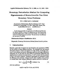
∗ Fig. 1. The kernels Kαβ (τ ) and their primitives Kαβ (τ ) in lin-log scales for Doppler profile.

We note here that the transformation of the vectorial transfer equation into a matrix equation is always possible (Ivanov 1995). When the primary source term S∗ (τ, µ) is not of the form ˆ A(µ) times a column vector, as in our two preceding examples, one writes the radiation field as the sum of a diffuse field (multiply scattered) and of a directly transmitted field (which satisfies Eq. (5) with S(τ, µ) replaced by S∗ (τ, µ)). The primary source term for the diffuse field has then the required form. 3. The generalized Lambda operator In this section we examine the properties of the operator Λ. In Sect. 3.1 we present some general comments on the solution of Eq. (29) that follow from the normalization and the behavior at ˆ ). In Sect. 3.2 infinity of the elements of the matrix kernel K(τ we calculate numerically the elements of the matrix corresponding to the operator Λ to examine its structure with respect to the Jacobi iterative method. 3.1. The propagating and mixing kernels The integral equation for the vector P or the matrix Sˆ can be written in the symbolic form P(τ ) = (1 − ε)Λ(P) + Q(τ ),

(29)

where Q(τ ) is a given primary source and Λ the integral operator in Eqs. (18) and (22) for T = ∞. In explicit form, the integral

Z

∞

K22 (τ − τ 0 )PQ (τ 0 ) dτ 0

0

Z

0

∞

K21 (τ − τ 0 )PI (τ 0 ) dτ 0 + QQ (τ ).

(31)

The four kernels Kαβ (τ ), α, β = 1, 2 are the elements of the ˆ defined in Eq. (19). Henceforth we use greek inmatrix kernel K dices to refer to the four elements of the (2×2) matrices involved in the polarized transfer equations. Following Ivanov (1995), we shall refer to the kernels K11 and K22 as the propagating kernels and to K12 as the mixing one. A slightly different version of the ˆ has been introduced in FSF for the case W2 = 1. Due kernel K to a different factorization of the phase matrix, the kernel in FSF F SF F SF = (9/8)K12 . The kernel K11 is not symmetrical and K21 has the same definition here and in FSF. For the other elements p F SF F SF . The and K22 = W2 K22 we have K12 = (3 W2 /8)K12 F SF explicit expressions of the Kαβ can be found in FSF. In Fig. 1 we show the three kernels and their primitives, Z ∞ ∗ Kαβ (u) du, (32) (τ ) = 2 Kαβ τ

for the case W2 = 1. All the elements, Kαβ (τ ), α, β = 1, 2, are even functions of τ . The propagating kernels K11 and K22 are positive and are normalized to 1 and W2 (7/10), respectively (the norm is the integral from −∞ to +∞). The mixing (coupling) kernel K12 = K21 has very different properties. Its integral over (0, ∞) is zero and as a consequence K12 takes both positive and negative values. There is only one change of sign which occurs around τ = 1, with K12 positive for smaller values of τ and negative for larger ones. Because we are dealing with complete frequency redistribution, the Kαβ (τ ) decrease algebraically to zero as τ → √ ∞. For a Doppler profile, for instance, they behave as 1/(τ 2 ln τ ). For τ → 0, they increase logarithmically. Asymptotic series valid at large and small τ can be found in FSF and in Ivanov et al. (1996a). It is interesting to discuss the properties of Eqs. (30) and (31), considered as two uncoupled scalar equations. The properties of Eq. (30), which has the same kernel normalized to unity as the standard integral equation for a scalar source function, are quite well known. In the limit of small ε, the characteristic scale of variation√of PI is given by the thermalization length which is of order (ε − ln ε)−1 for a Doppler profile, and of order aε−2 for a Voigt profile with parameter a. At large depths, PI behaves as the inhomogeneous term divided by ε, provided this term is also slowly varying. Equation (31) is somewhat different since the kernel K22 is normalized to W2 (7/10). However we can easily recast it in a standard form by a simple redefinition of the

M. Faurobert-Scholl et al.: An operator perturbation method for polarized line transfer. I

˜ 22 = K22 /W2 (7/10) which is kernel. Introducing the kernel K then normalized to unity, we can rewrite Eq. (31) as Z ∞ ˜ 22 (τ − τ 0 )PQ (τ 0 ) dτ 0 + PQ∗ (τ ), K ˜ (33) PQ (τ ) = (1 − ε) 0

with 7 1 − ε˜ = W2 (1 − ε). 10

(34)

Ivanov (1995) has introduced the notation εQ for ε. ˜ The inhomogeneous term PQ∗ (τ ) is the sum of the coupling term and of the primary source QQ (τ ). For ε  1, one has ε˜ ' W2 (3/10). So the effective destruction probability is fairly large. As a result PQ (τ ) will not depart very strongly from the inhomogeneous term PQ∗ (τ ). For instance at large τ , one has

901

Here E is the identity operator. The operator A involves three linear operators : the operators A11 and A22 which are defined by Z ∞ Aαα f (τ ) = f (τ ) − (1 − ε) Kαα (τ − τ 0 )f (τ 0 ) dτ 0 , (39) 0

for α = 1, 2 and the operator A12 defined by Z ∞ A12 f (τ ) = −(1 − ε) K12 (τ − τ 0 )f (τ 0 ) dτ 0 .

(40)

0

(35)

Because K12 = K21 , we have A12 = A21 . In the subsequent equations, we use only A12 . A discretization of the τ variable (τ = {τi }, i = 1, N ) transforms the operators Aαβ into square matrices : X Aαβ f (τ ) → Aαβ (i, j)fj , i = 1, N, (41)

Numerical solutions of Eq. (33) show that this relation is well satisfied when τ > 10. Another consequence of the relatively large value of ε˜ is that a Neumann series expansion of PQ (τ ) will be rapidly convergent. We consider now the coupling terms. To understand the effect of a convolution by K12 , let us assume that K12 acts on a constant C. One has Z ∞ 1 ∗ C (τ ), (36) K12 (τ − τ 0 ) dτ 0 = − CK12 2 0

with fj = f (τj ). Note that we shall be using the same notation for the integral operator and the corresponding matrix. Roman letters are used to denote indices corresponding to the optical depth grid. The choice of the grid and of the representation of f (τ ) does affect the numerical values Aαβ (i, j) but not the global properties that are discussed here. For non-polarized problems, as already shown in OAB the matrix A11 is diagonally dominant, i.e. satisfies the criterion X |A11 (i, k)|, i, k = 1, N, (42) |A11 (i, i)| ≥

PQ (τ ) '

10 ∗ 1 ∗ P (τ ) = P (τ ). ε˜ Q 3W2 Q

∗ (τ ) is the primitive of K12 (τ ) defined in Eq. (32). The where K12 ∗ (τ ) is negative for all τ , goes to zero for τ → 0 and function K12 −2

τ → ∞. Its absolute value has a maximum around 6 × 10 at τ ' 0.75 (see Fig. 1). The convolution of a constant with K12 leads thus to a function which has a maximum at optical depths around one and which is more than ten times smaller than the original function. The functions PI (τ ) and PQ (τ ) are of course not independent of τ unlike C but the behavior found above is very typical of the action of K12 . The weakness of the coupling term in the equation for PI (τ ) and the normalization of K22 to a value significantly smaller than unity explain the success of the perturbation methods mentioned in the Introduction. In a first step one solves the non-LTE problem for the intensity, neglecting the polarization, and then calculates the polarization by an iterative procedure which amounts to a Neumann series expansion of Eq. (31). One then corrects the intensity for the polarization and iterates until convergence. 3.2. The propagating and mixing operators It is convenient to rewrite Eq. (29) for P in the form A(P) = Q(τ ),

(37)

where A = [E − (1 − ε)Λ].

(38)

j

k/ =i

but what about A22 and A12 ? The criterion (42) is presented with more detail in Appendix A. We stress that it is a sufficient but not a necessary condition for the convergence of the Jacobi iterative method. To analyze the structure of the matrices Aαβ , we have calculated their elements numerically by the method which is described below. The iterative technique described in Sects. 4 and 5 however, makes use only of the diagonal elements of these matrices. The results presented in this section have been obtained with a Doppler profile and W2 = 1. To calculate the kernels Kαβ , we have used the representation by Pad´e approximants established in Hummer (1981) for K11 and in FSF for K22 and K12 . It has been noticed by Ivanov et al. (1996b) that there is a printing er∗ : the last three significant digits ror in the coefficient p8 of K22 should be 649 and not 465. A mixed quadratic-linear representation is used for f (τ ). For a given grid point τi , we assume for f (τ 0 ) a parabolic representation in the interval [τi−1 , τi+1 ] and a linear representation outside this interval. The asymptotic analysis of the operator A11 (Frisch & Frisch 1977, Frisch & Froeschl´e 1977) shows that it is necessary to ensure the continuity of the first derivative of f (τ 0 ) in an interval centered around τ 0 = τi , especially for a Doppler profile. The accuracy of this representation has been examined by Bommier & Landi degl’Innocenti (1994, 1996) and is typically around 2%. In the lower panels of Figs. 2 and 3 we show the diagonal elements Aαβ (i, i) and rows of Aαβ , i.e. Aαβ (i, j) for some

902

M. Faurobert-Scholl et al.: An operator perturbation method for polarized line transfer. I Matrix A11 10

20

30

40

10

50

0

20 30

50

0 -0.04

20 30 40

40

50

50 10

20 30 40 grid index j

50

10

20 30 40 grid index j

50

0.8

0.8

A22(i,i)

A11(i,i) 0.6

0.6

A22(i,j)

A11(i,j)

40

10

-0.04

grid index i

grid index i

10

Matrix A22 20 30

0.4 0.2

0.4 0.2

0.0

0.0

-2

-1

0

1

2

3

-2

Log τ

-1

0

1 Log τ

selected values of i and all values of j. The upper panel shows 2D contours of Aαβ (i, j). The upper left corner corresponds to the element Aαβ (1, 1) and the lower right corner to Aαβ (N, N ), with N the total number of depth points. Fig. 3 actually shows −A12 (i, j). The figures have been produced with 10 grid points per decade for τ between 10−2 and 103 . The correspondence between the grid index g and the optical depth τ is thus g = 10 log10 τ + 20. For A11 and A22 , Fig. 2 shows that the largest element, for any row, lies on the diagonal. For A11 the diagonal elements go to ε at large optical depths and for A22 they go to 3/10. These values determine the asymptotic behavior of PI (τ ) and PQ (τ ) at large τ (see above). To examine the question of diagonal dominance, we have calculated numerically the ratio λαα = max{ i

X k/ =i

|Aαα (i, k)|/|Aαα (i, i)|},

α = 1, 2.

(43)

For a grid spacing with 8 points per decade we find λ11 = 0.95 and λ22 = 0.48. We can conclude that A22 is also diagonally dominant and that the spectral radius (see Varga 1962 or Appendix A for a definition) of the corresponding amplification matrix is significantly smaller for A22 than for A11 . For A11 , the ratio in Eq. (43) has its maximum value around τi = 32 and for A22 around τi = 1.5. The values of λαα are grid dependent (they increase when the grid becomes finer) but the position of the maximum is essentially independent of the grid. In Fig. 3, we can note that the diagonal elements of −A12 have a maximum of the order of 6 × 10−2 around τ = 4. This ∗ . For τ → 0 value is of the same order as the maximum of −K12 and τ → ∞, the diagonal elements go to zero. We find that the

2

3

Fig. 2. Behavior of the matrix (operator) Aαα = E − (1 − ε)Λαα . Upper panels : 2D contours of the entries Aαα (i, j). Lower panels : Diagonal elements Aαα (i, i) (smooth curve) and elements Aαα (i, j) for selected values of the row index i and all values of j. For each row i, the abscissa of the largest element yields the corresponding optical depth since the largest element is on the diagonal. For τ → ∞, the diagonal elements of A11 and A22 go to ε and 0.3, respectively.

value of λ12 is largely above unity. Clearly A12 is not diagonally dominant. The broad white–grey portion on the top left corner in the upper panel roughly corresponds to optical depths where the ratio in Eq. (43) is larger than unity. For rows of index less than 3, the diagonal element is even not the largest. The full matrix A has a block structure since each “element” is a (2 × 2) matrix. The above analysis has shown us that the two propagating operators A11 and A22 are diagonally dominant and that the mixing operator A12 is not. As for the full matrix A, it does not satisfy the criterion (42) for 3 < τ < 103 . This is roughly the region where A11 barely satisfied the criterion (42). However, the standard (point) Jacobi method is convergent. We have already pointed out that diagonal dominance is not a necessary criterion for convergence. We have found that convergence is somewhat faster if in place of the point Jacobi method, we use a block Jacobi iterative method where the approximate transport operator is a block diagonal matrix with elements dii defined by   A11 (i, i) A12 (i, i) . (44) dii = A12 (i, i) A22 (i, i) In terms of the operator Λ,   1 − (1 − ε)Λ11 (i, i) −(1 − ε)Λ12 (i, i) . dii = −(1 − ε)Λ12 (i, i) 1 − (1 − ε)Λ22 (i, i)

(45)

The iterative method, its implementation and convergence tests are described in the next section in the framework of the matrix integral equation (22). From a computational point of view it is more convenient to work with the matrix formalism ˆ ) and S(τ ˆ ) satisfy Eq. (20). because the four elements of I(τ

M. Faurobert-Scholl et al.: An operator perturbation method for polarized line transfer. I 10

30

20

40

grid index i

ˆ ) with the integral equation Comparing the definition of S(τ ˆ satisfied by S(τ ) (see Eqs. (21) and (46)) we see that

50

0.02 0 -0.004

10

Λ(Sˆ (n) )(τ ) = Jˆ(n) (τ ),

(50)

20

with

30

ˆ )= J(τ

40

10

20 30 40 grid index j

50

0.060 0.050 0.040

A12(i,i)

0.030 0.020 0.010 0.000 -0.010 -2

Z

+∞

−∞

50

A12(i,j)

903

-1

0

1 Log τ

2

3

Fig. 3. Behavior of the matrix (operator) −A12 = (1 − ε)Λ12 . See the caption of Fig. 2. The diagonal elements (bell shaped curve in the lower panel) go to zero for τ → ∞.

4. An approximate Lambda iteration method for polarized transfer 4.1. Implementation of the iterative method We consider the integral equation (22) which we write in the symbolic notation ˆ + Sˆ ∗ . Sˆ = (1 − ε)Λ(S)

(46)

ˆ denoted by Sˆ (n) . Let us assume that we know an estimate of S, At iteration (n + 1) we write ˆ Sˆ (n+1) = Sˆ (n) + δ S.

(47)

The correction term obeys the equation ˆ = −A(Sˆ (n) ) + Sˆ ∗ A(δ S)

(48)

with A = [E − (1 − ε)Λ] and E the identity operator. We now replace in the l.h.s. of Eq. (48) the matrix A by the block diagonal matrix D = {dii } introduced in Eq. (44). Expressing in the r.h.s. of Eq. (48) the matrix A in terms of Λ, we obtain for each optical depth grid point, ˆ i ) = d−1 [(1 − ε)Λ(Sˆ (n) )(τi ) − Sˆ (n) (τi ) + Sˆ ∗ (τi )]. δ S(τ ii

(49)

Each term in this equation is a (2 × 2) square matrix. The matrices dii and Λ(Sˆ (n) )(τi ) can be calculated as shown below by integrating the radiative transfer equation (20) with given maˆ ). trices S(τ

0

φ(x )

Z

+1

−1

0

ˆ 0 )I(τ, ˆ x0 , µ0 ) dµ dx0 . (51) Aˆ T (µ0 )A(µ 2

The matrix Jˆ(n) is the frequency and angle averaged intensity for polarized problems. Knowing Sˆ (n) (τ ) we calculate Iˆ(n) (τ ) with Eq. (20), using a Feautrier formal solution method and then integrate over frequencies and directions as shown in Eq. (51). To ensure that the iterative method converges to the solution of the actual problem, the matrix in the square bracket of Eq. (49) must be calculated very accurately. This requires a preconditioning of the transfer equation to avoid round–off and truncation errors in the calculation of the differences Jˆ(n) (τi ) − Sˆ (n) (τi ) (see e.g., Rybicki & Hummer 1991). Actually the difficulty arises only at large optical depths for the element {11} and is due to the normalization to unity of the kernel K11 . The matrices dii are calculated once for all by solving Eq. (20) with   ˆ ) = δ(τ − τi ) 1 0 , (52) S(τ 0 1 where δ is the Dirac distribution. For this source matrix, as shown by Eq. (50), Λαβ (i, i) = Jαβ (τi ). The elements of dii can then be calculated from Eq. (45). In the vector formalism, two different vectorial source terms : P(τ ) = δ(τ − τi )(1, 0)T and P(τ ) = δ(τ − τi )(0, 1)T are needed to calculate the matrices dii . The first expression yields Λ11 (i, i) and Λ21 (i, i) and the second one Λ12 (i, i) = Λ21 (i, i) and Λ22 (i, i). Computational details For the optical depth grid we use 8 points per decade. We stress that the grid spacing determines both the accuracy of the result and the speed of convergence of the iterative method. Roughly speaking, the coarser is the grid, the faster is the convergence. We can understand this trend in the following way: the “local” approximation of the operator Λ represents the radiative interactions in the neighborhood of each depth point τi , i.e. in between τi−1 and τi+1 . The extent of this region is larger if the optical depth grid is not too fine. Indirectly, the long distance interactions are then better represented. The effects of the grid spacing and of other parameters such as ε and the optical thickness of the medium on the rate of convergence have been studied in detail in the case of scalar problems (e.g. OAB, Auer et al 1994; Trujillo Bueno & Fabiani Bendicho, 1995). Having found essentially the same effects for our vectorial/matrix problem, we refer the reader to the articles listed above. For the frequency grid, we use a two-point Gauss formula, per decade of the profile function φ. The maximum value of the

M. Faurobert-Scholl et al.: An operator perturbation method for polarized line transfer. I

frequency, xm , is chosen such that T φ(xm ) ' 10−2 , with T the total optical thickness of the medium. Because the calculation of Jˆ(n) (τ ) involves 2nd–order moments of Iˆ(n) (τ ), the angular grid must be sufficiently fine. After a few tests, we have retained a three-point Gauss formula for µ ∈ [0, 1]. It yields an error of order of 5% on the polarization and 1% on the intensity with respect to a 9-point formula.

2

log10(Max Rel. Correction)

904

0 -2 21 -4 -6 -8

4.2. Test problems

∗ S22 (τ ) = 0.

(53)

Thus only the elements of the first column of Sˆ (i.e. S11 and S21 ) are different from zero. In case (ii), the internal thermal emission is zero but there is at each surface an incident field of the form Iinc = δ(µ ∓ µo )I inc (1, pinc )T ,

(54)

where ∓µo , (µo > 0) are the directions of the incident beam at τ = 0 and τ = T , respectively. Combining Eqs. (13) and (26) to (28), we find ∗ S11 (τ, µo ) =

1 − ε inc I [M (τ, µo ) + M (T − τ, µo )] 2

(55)

and ∗ (τ, µo ) S22

=

r

W2 ∗ [(1 − 3µ2o ) + 3pinc (1 − µ2o )]S11 (τ, µo ).(56) 8

ˆ i.e. S12 and S22 , Only the elements of the second column of S, inc depend on the polarization p of the incident radiation. All the calculations have been carried out for a Voigt absorption profile with a = 10−3 and a depolarization parameter W2 = 1. The medium is characterized by the total frequency averaged line optical thickness T and the destruction probability ε. All the results shown here correspond to T = 2 × 109 and ε = 10−6 . For the self-emitting slab, B = 1. For the illuminated slab, B = 0, µo = 0.5, I inc = 1 and pinc = −20%. 4.3. Behavior of the correction terms We examine in this section the behavior of the corrections δ Sˆ αβ as one advances in the iteration process, postponing to Sect. 4.6 the discussion on the convergence criterion. The relevant quantities for this study are the maximum of the relative corrections (n) (n+1) c(n) αβ = max{|δSαβ (τi )/Sαβ (τi )|}. τi

(57)

log10(Max Rel. Correction)

50

In this paper we consider two different problems, (i) a selfemitting slab with a uniform temperature, (ii) a slab illuminated on both sides by an exterior radiation field. In our two examples the slab is symmetric with respect to the mid-plane. We have computed the radiation field in one half of the slab only, by imposing that the derivatives of the four elements of the matrix radiation field are zero at mid-plane. In case (i), ∗ (τ ) = εB; S11

11

100 150 iteration number

200

0 12 11 21

-5

22

-10

50

100

150

200

iteration number

Fig. 4. Maximum relative corrections c(n) αβ as function of the iteration number in lin-log scales for a slab with T = 2 × 109 , ε = 10−6 and a = 10−3 . Upper Panel : self-emitting slab with B = 1. Lower Panel : illuminated slab with I inc = 1, pinc = −20%, and B = 0. Note that the curves in the upper and lower panels have the same slope at large n.

They are shown in Fig. 4, as function of iteration number n, for the two test problems defined above. The stopping criterion −2 −8 for all α and β. corresponding to Fig. 4 is c(n) αβ ≤ 10 ε = 10 Figs. 6 and 7 show the convergence history of the source matrix elements Sαβ (τ ) after application of the Ng acceleration procedure discussed in Sect. 4.4. To start the iteration cycle we have chosen Sˆ equal to the primary source term Sˆ ∗ . The converged solution satisfies the set of equations A11 (S11 ) + A12 (S21 ) A22 (S21 ) + A12 (S11 ) A11 (S12 ) + A12 (S22 ) A22 (S22 ) + A12 (S12 )

= = = =

∗ S11 , 0, 0, ∗ S22 .

(58) (59) (60) (61)

Fig. 4 shows that c21 for the self-emitting slab (upper panel) and c12 for the illuminated slab (lower panel), go through sharp maxima at the beginning of the iteration procedure. For scalar transfer problems, the source function is always positive. Here the elements S21 for the self-emitting slab and S12 for the illuminated slab have a change of sign (see Figs. 6 and 7). The sharp maxima in the maximum relative corrections appear whenever the depth point where the change of sign occurs is very close to a grid point. The corrections c21 and c12 start to decrease smoothly when this point does not move spatially from one iteration to the other. To avoid these peaks in the iteration process, which have no special meaning, and can even be a real nuisance if the zero of the converged solution happens to be very close to a

M. Faurobert-Scholl et al.: An operator perturbation method for polarized line transfer. I

0 -2 S11

log10(Max Rel. Correction)

10

21

-4 -6

0

10

-1

10

-2

10-3 10

11

905

-4

10-5 10

-8

-6

-2

50

100

150

0

2 Log τ4

6

8

0

2

6

8

200

iteration number

0

-2 -5

0 -2

S21/ 10

log10(Max Rel. Correction)

-1

-4 11 21

-6

-6 -7 -2

22

-12 50

100

-4 -5

12

-8 -10

-3

150

200

iteration number

Fig. 5. Effect of Ng acceleration. Solid line : maximum relative corrections c¯(n) αβ . Dotted line : same quantities with Ng acceleration. Same values of the model parameters as in Fig. 4 are employed. Upper Panel : self-emitting slab. Lower Panel : illuminated slab.

grid point, it seems preferable to define the maximum relative corrections with the modified formula ) ( (n) |δSαβ (τi )| (n) . (62) c¯αβ = max 1 (n+1) (n+1) τi 2 [|Sαβ (τi )| + |Sαβ (τi+1 )|] Fig. 5 shows the variation of the c¯(n) αβ with n. Differences be(n) (n) tween c¯αβ and cαβ appear only at the beginning of the iterations. They essentially disappear for large values of n. Another striking feature of Fig. 4 is that all the cαβ have the same rate of decrease at large n. The numerical results give ln c(n) αβ ∼ n ln |λ1 | with |λ1 | = 0.916 ± 0.005. This value is controlled by the operator A11 . We give a simple model in Appendix B to explain this behavior. We can also understand it directly from Eqs. (58) to (61). In Eq. (58), the coupling term ∗ A12 (S21 ) is negligible compared to the primary source term S11 (see Sect. 3.1). Therefore the rate of decrease of c11 is determined by the largest eigenvalue (in modulus) of the amplification matrix F11 , corresponding to A11 . Its value, 0.916, is consistent with the upper bound λ11 = 0.95 given in Sect. 3.2. For c22 (see lower panel) we observe a larger rate of decrease at the beginning of the iterations. At the start of the iteration process, the rate of decrease of c22 is controlled by the operator A22 because the coupling term A12 (S12 ) in Eq. (61) is negligible ∗ (we start the iterations with S12 = 0). We have compared to S22 shown in Sect. 3.2 that λ22 , the upper bound for the eigenvalues of the amplification matrix corresponding to A22 , is smaller than

Log τ

4

Fig. 6. Convergence history of the source function elements Sαβ (τ ) for a self-emitting slab with B = 1, T = 2 × 109 , ε = 10−6 and a = 10−3 . The dotted lines show the initial solutions which are equal to εB for S11 (τ ) and to 0 for S21 (τ ). Upper panel S11 (τ ) in log-log scales. Lower panel S21 (τ ) in log-lin scales.

λ11 . Hence the observed phenomenon. When the mixing term A12 (S12 ) becomes relevant, the rate of decrease of c22 becomes equal to the rate of decrease of c12 which is also determined by |λ1 | since the transport operator acting on S12 is A11 . For S21 , the transport term is controlled by A22 but the coupling term by A11 through S11 . It is the latter, because it decreases more slowly, which dominates at large n. We can summarize this discussion, by saying that S12 , S21 and S22 are slave modes of S11 at large n. 4.4. Ng acceleration In the scalar case, several techniques have been proposed to accelerate the speed of convergence of ALI methods, the most commonly used ones are the Ng acceleration technique and the orthomin method (see Auer 1991 for a review). A recent investigation (Auer et al. 1994) shows that they have essentially the same effect. Since the memory requirement for the Ng technique is significantly smaller than for the orthomin method, we have retained the former one. Ng acceleration is applied separately ˆ to each element of the matrix S. Fig. 5 shows the dependence on n of the c¯(n) αβ , without and with the Ng acceleration. In this acceleration procedure, every fourth iteration the source function is replaced by a linear combination of the 3 previous iterations. The coefficients are (n) calculated in order to minimize the “distance” between Sαβ (n+1) and Sαβ (see OAB). The distance is defined as the sum over all the depth points of the squared difference between these two functions, multiplied by a positive weight. For the 11-element

906

M. Faurobert-Scholl et al.: An operator perturbation method for polarized line transfer. I

0 1.0 -1 -3

0.8

S12 / 10

S11

0.6 0.4

-3 -4

0.2 0.0 -2

-2

-5 0

2

Log τ

4

6

8

-2

7

0

2

Log τ

4

6

8

0

6 -1

4

S22 / 10-2

S21 / 10-2

5

3

-2 -3

2 -4

1 0 -2

0

2

Log τ

4

6

8

-5 -2

0

2

we employ the same weight as in OAB, i.e. W11 (τi ) = 1/S11 (τi ) so that the region of small optical depths where S11 (τ ) is small is properly taken into account. For the other elements, we simply use Wαβ (τi ) = 1. A delayed start of Ng when the maximum error becomes smaller than 1, as sometimes advocated (Rybicki and Hummer 1991), does not improve the convergence. The Ng acceleration is always started at the fourth iteration and applied each fourth iteration. We have not tried to increase the number of regular iterations between an application of the Ng extrapolation scheme, since there does not seem to be much to gain (Auer et al. 1994). We see that the effect of the Ng method is to accelerate the convergence by a factor 3 to 4. For S11 , each application of the Ng acceleration produces a decrease in the correction term. For the other elements, the readjustment occurring at the iteration following the Ng extrapolation produces an increase in the correction term which is due to the fact that the Ng extrapolated values are not consistent with the transfer equation. The overall convergence is however almost the same for c¯(n) 11 and the other (see Fig. 5). c¯(n) αβ 4.5. Some comments on the solution of the test problems Figs. 6 and 7 show the convergence history of the elements of the source matrix after application of the Ng acceleration. One easily sees the effect of the Ng extrapolations every fourth iteration. After convergence, these elements satisfy Eqs. (58) to (61). We also recall that they are related to the components of the vector source function P(τ ) by Eq. (4), which we can write as PI (τ ) = S11 (τ ) + S12 (τ ),

Log τ

4

6

8

Fig. 7. Convergence history of the source function elements for a slab illuminated by an incident polarized radiation field of intensity I inc and polarization pinc = −20%. Same slab parameters as in Fig. 6 with B = 0. The dotted lines show the initial solutions. All the elements Sαβ (τ ) are in log-lin scales. Only one half of the slab is represented because the slab is symmetric about the mid-plane.

PQ (τ ) = S21 (τ ) + S22 (τ ).

(63)

We first consider the self-emitting slab. In this case S11 (τ ) = PI (τ ) and S21 (τ ) = PQ (τ ) (the second column of the matrix source function is zero). The element S11 (τ ) is essentially identical to the non–polarized scalar source function S(τ ) because the mixing term is negligible compared to the primary source ∗ (τ ). We note that S11 (τ ) is almost thermalized to the term S11 Planck function but not fully (its value is slightly under unity at mid-slab), because the thermalization length aε−2 is of the order of the actual slab thickness. The surface value is essentially governed by the exact result (Ivanov 1990) PI2 (0) + PQ2 (0) = εB,

(64)

which holds for a semi-infinite medium with a uniform primary source εB, with B = (B, 0)T . Since PQ (0) is very small √ compared to PI (0), one has, as shown in Fig. 6, S11 (0) ' εB. The element S21 (τ ) has values of the order of magnitude of −A12 (S11 ) as seen from Eq. (59). At small optical depths one ∗ (τ )S11 (0). Since S11 (0) ' 10−3 , this has thus S21 (τ ) ' −K12 yields S21 (τ ) of the order of 10−5 at the surface. We note also that S21 (τ ) has a change of sign. One can verify that it coincides with a change in the anisotropy of the radiation field which goes from limb darkening to limb brightening when the optical depth increases inward from the surface. We now consider the case of the illuminated slab. Because ε is very small and the slab thickness is of the same magnitude as the thermalization length, the slab is almost totally reflecting. As a result S11 (0) ' I inc and the influence of the incident polarized radiation field on S11 (τ ) is felt over most of the slab (note the linear scale for S11 (τ ) in Fig. 7). In contrast, the polarization

M. Faurobert-Scholl et al.: An operator perturbation method for polarized line transfer. I

0.05 S21

0.00 PQ

-0.05 -2

S22 0

2

4 Log τ

6

8

Fig. 8. The illuminated slab. The matrix elements S21 (τ ), S22 (τ ) and their sum PQ (τ ) are shown as function of optical depth in log-lin scales.

stays concentrated near the surface because a large number of scatterings act efficiently to destroy polarization in the deeper layers. For the element S21 (τ ), the argument developed above leads ∗ (τ ). Hence, at the surface S21 (τ ) of the order to S21 (τ ) ' −K12 −2 of 10 . The element S12 (τ ) is negligibly small at all depths compared to S11 (τ ) because of the smallness of the coupling term A12 (S22 ) (see Eq. (60). ∗ Finally we remark that S22 is of the order of S22 . There are two reasons for this behavior, the mixing term A12 (S12 ) (see ∗ and Eq. (61)) is negligible compared to the primary source S22 A22 has an interaction range of order unity. We show in Fig. 8 the elements S21 (τ ) and S22 (τ ) and their sum PQ (τ ) which is the relevant physical quantity for the polarization component. Concerning the illuminated slab, one may raise the question whether the convergence of the iterative process should ˆ ) or only on be tested on the four elements of the matrix S(τ the physical quantities PI (τ ) and PQ (τ ) (see Eq. (63)). For the intensity component, S12 (τ ) is negligible compared to S11 (τ ). Therefore it is sufficient to test their sum for convergence. Since (n) c¯(n) 12 ≈ 10 c¯11 , testing PI (τ ) will save a number of iterations. For the polarization component, S21 (τ ) and S22 (τ ) are of the same order, with S21 (τ ) positive for all τ and S22 (τ ) negative for all τ . Their sum PQ (τ ) shown in Fig. 8 has a change of sign. As a consequence, the maximum relative correction for PQ (τ ) (not shown in Figs. 4 nor 5), oscillates at the beginning of the iterations and is larger than c¯(n) 21 . For the polarization component, it thus appears preferable to apply the convergence criterion to S21 (τ ) and S22 (τ ) separately. This is an advantage of the matrix formulation over the vector formulation. 4.6. Convergence criterion A stopping criterion for the iterative procedure, commonly used for scalar transfer problems (see e.g. Auer & Paletou 1994) is c(n) ≤ 10−2 ε. The same criterion is applied by us to each of the c¯(n) αβ to produce Figs. 4 and 5. Recently Auer et al. (1994) have pointed out that the converged solution for a grid with a

907

given spacing contains a built-in truncation error, with respect to the true solution that could be obtained on a grid with infinite resolution, and they stress that it is a waste of computing time to approach the converged solution corresponding to a given grid with an accuracy which is larger than that of the converged solution itself. For polarized transfer, as discussed in Sect. 4.5, the relevant quantities for testing the convergence of the method are the source function PI (τ ) for the intensity and, depending whether the primary source is polarized or not, the matrix elements S21 (τ ) and S22 (τ ), or the source function PQ (τ ) for the polarization. We now discuss the new convergence criterion suggested by Auer et al. (1994) for the case of the self-emitting slab transfer problem. The relevant quantities for the convergence test are the intensity and polarization source functions PI (τ ) = S11 (τ ) and PQ (τ ) = S21 (τ ). The test introduced by Auer et al. (1994) involves three quantities which are defined below and plotted in Fig. 9. The first one is the maximum relative correction, already introduced in Sect. 4.3, which we write here as (n) (n+1) ¯ (n) c¯(n) I,Q (g) = max[|PI,Q (g) − PI,Q (g)|/PI,Q (g)]. τ

(65)

The subscripts I and Q refer to the intensity and polarization (n) (g) stands for the denominator in Eq. (62) and component, P¯I,Q g is an index indicating the level of spatial resolution of the optical depth grid. We adopt the convention of Auer et al. (1994) that the larger is the index g the finer is the grid. The second quantity of concern is the maximum relative convergence error, (∞) (n) ¯ (∞) e(n) I,Q (g) = max[|PI,Q (g) − PI,Q (g)|/PI,Q (g)], τ

(66)

where n = ∞ indicates that one is dealing with the fully converged solution on grid g. The third quantity is the maximum truncation error, (∞) (∞) (n) (n) (∞)], (∞)|/P¯I,Q (g) − PI,Q (g) = max[|PI,Q EI,Q τ

(67)

where g = ∞ indicates the true solution on a grid of infinite resolution. To determine the convergence and the truncation errors (∞) we have calculated the converged solution PI,Q (g) and the true (∞) solution PI,Q (∞) with a non iterative Feautrier method, using 8 and 16 depth points per decade, respectively. The angle and frequency grid points employed for the direct Feautrier solution are the same as for the iterative method. An elegant method for estimating the true error, based on a grid doubling strategy, is described in Auer et al. (1994). Fig. 9 shows that the maximum relative correction c¯(n) I,Q (g) (also plotted in Fig. 5, upper panel) goes to zero when n goes to infinity and that the maximum relative error e(n) I,Q (g) has the (n) same rate of decrease as c¯I,Q (g) before it reaches a constant value. In the scalar case, Auer et al. (1994) have shown that e(n) (g) ≈ c(n) (g)

|λ| , |1 − λ|

(68)

where λ is the eigenvalue which controls the rate of convergence. This relation is obtained by writing that the converged solution

908

M. Faurobert-Scholl et al.: An operator perturbation method for polarized line transfer. I

satisfies Eq. (A5). One can verify, using |λ1 | ' 0.916, that the relation (68) holds in the case at hand for both PI (τ ) and PQ (τ ). The relation (68) predicts that e(n) (g) goes to zero for n going to infinity. Here, it goes to a constant of order 10−6 for the intensity component and of order 10−4 for the polarization (∞) (g) component. The reason is simply that we have used for PI,Q the solution given by a direct Feautrier method, and not the converged solution of the iterative process. Differences between these two solutions are to be expected since they are obtained with different numerical methods involving different levels of truncation errors in the algorithms. For instance, the Feautrier method requires the inversion of large (2Nt × 2Nt ) matrices, with Nt being the product of the number of directions by the number of frequencies. (n) (g) goes to a conWhen n goes to infinity, the true error EI,Q (∞) stant EI,Q (g) which measures the error between the converged solution and the true solution. Fig. 9 shows that one introduces a 1% error on the intensity component and a 5% error on the polarization component when the grid spacing goes from 16 depth points per decade to 8 depth points per decade. The suggestion of Auer et al. (1994) is to stop the iterative process when the maximum relative error becomes smaller than the true error. Here this criterion becomes (∞) e(n) I,Q (g) < EI,Q (g),

(69)

for both the I and Q component. To apply this criterion one (∞) (g) and the variation with needs a method for estimating EI,Q (n) n of the maximum relative error eI,Q (g). The latter can be deduced from the iterative process itself which yields both |λ1 | (n) and c¯(n) I,Q (g) and hence eI,Q (g) with the help of Eq. (68). For the −3 and example of Fig. 9, the criterion (69) leads to c¯(n) I < 10 (n) −2 c¯Q < 10 . Fig. 5 (upper panel) shows that it is satisfied after just 30 iterations, if the Ng acceleration procedure is applied. 4.7. CPU requirements Using the matrix formalism developed by Ivanov (1995), we have shown that the Jacobi-type ALI method introduced by OAB for scalar problems can be generalized to vectorial problems such as resonance polarization of spectral lines. To demonstrate the usefulness of the PALI method, we still have to show that it offers a significant gain in computing time with respect to a direct method of solution, say, of the Feautrier type. Let Nν and Nµ be the number of frequency and angle points. For the Feautrier method, the computing time increases as Nt3 and the memory space as Nt2 where Nt = Nν Nµ . In ALI methods, they both increase linearly with Nt . In Table 1 we compare various computing times for our reference self-emitting slab problem. The calculations have been performed on a Sun 670 −8 MP workstation with a stringent stopping criterion, c¯(n) αβ < 10 for all α and β. It is clear that the advantage of the PALI method is overwhelming when a large number of frequency points is required for a given problem. The Ng acceleration reduces the computing time by a factor of 2 although the number of iterations needed to reach the stopping criterion is cut down by a

Intensity 0

10 10

-1 (n) I

E

10-2 10

-3

10

-4

10-5 10

-6

10

-7

10

-8

10-9

(n) I

e

(n) I

c 50

Polarization

101 10

100 150 200 iteration number

0

10

-1

10

-2

E(n)Q

10-3

e(n)Q

10-4 10-5 10

-6

10

-7

10

-8

(n) Q

c 50

100 150 200 iteration number

Fig. 9. Maximum of the relative corrections c¯(n) I,Q , of the relative errors (n) (n) eI,Q and of the true errors EI,Q as functions of the iteration number for the self-emitting slab transfer problem. Upper Panel : intensity component. Lower Panel : polarization component. Table 1. CPU time requirements. Self-emitting slab with T = 2 × 109 , ε = 10−6 , a = 10−3 , Nµ = 3 and 8 depth points per decade. Method Feautrier PALI PALI + Ng

Nν = 20 97s 25s 14s

Nν = 30 345s 48s 23s

Nν = 50 2300s 93s 43s

factor of 3-4. Every fourth iterations some CPU time is spent in the calculation of the coefficients of the linear combination used for the Ng acceleration. In the light of the discussion presented in Sect. 4.6, a softer stopping criterion is suitable for the PALI method also. In that case, the CPU requirements of PALI will be even less than what is given in Table 1. 5. Conclusions In this paper we have introduced an Approximate Lambda Iteration method of the block-Jacobi type for non-LTE polarized transfer (PALI). The iterative scheme has been developed using the formalism of the matrix transfer equation introduced by Ivanov (1995), which appears ideal for the generalization of operator splitting techniques to polarized transfer problems. We have tested the method on two standard problems in strongly non-LTE conditions : a self-emitting slab and a slab illuminated

M. Faurobert-Scholl et al.: An operator perturbation method for polarized line transfer. I

by a polarized radiation field. The convergence and accuracy aspects of the PALI method have been analyzed in terms of the asymptotic properties of the amplification matrix. It was necessary to introduce a new definition for the maximum relative correction which serves to follow the convergence of the iteration process, because the Stokes parameters for the polarization are not always positive quantities unlike the scalar intensity. We also suggest a convergence (or stopping) criterion for PALI, based on the recent work of Auer et al. (1994) on scalar Approximate Lambda Iteration methods. Our PALI method is simple to code, and in its present form can handle axisymmetric situations, including Hanle depolarization by turbulent magnetic fields. The gain in computing time and memory over standard non-iterative methods, makes it a method of choice for extensions to multi-dimensional geometries. Acknowledgements. The authors are indebted to V. Bommier and V.V. Ivanov for very constructive remarks on a first version of the manuscript and to P.L. Sulem for interesting discussions on the convergence properties of matrix iterative methods. They are also grateful to V.V. Ivanov for informing them of an unpublished work on an iterative method for solving the integral equation for the polarized matrix source function (Nikolaev 1992; diploma work, St. Petersburg University). K.N.N. would like to thank the Observatoire de la Cˆote d’Azur and H.F. the Weizmann Institute of Sciences (Department of Chemical Physics) and Princeton University (Fluid Dynamics Research Center) for their kind hospitality during the course of this work.

909

never to be calculated. Equation (A4) also shows that the Jacobi method, as all the other operator splitting methods, amounts to making an estimation of the corrective term. The rate of convergence of any iterative procedure is controlled by the spectral radius of the amplification matrix ρ(F ) = max |λi |, i

(A6)

where the λi are the eigenvalues (real or complex) of the matrix F (Varga 1962). We deduce from Eq. (A5) that ∆x(n) = F ∆x(n−1) . Hence, asymptotically for large n, ∆x(n) ' λmax ∆x(n−1) ,

(A7)

with λmax being the complex eigenvalue of F with the largest modulus (or absolute value if the λi are real) (Puls & Herrero 1988). This asymptotic relation shows that |λmax | < 1 is a necessary condition for the convergence of the iterative process; that smaller the |λmax |, the faster is the convergence; that |λmax | can be deduced from the iterative process itself, and finally that the relation ln |∆x(n) | ∼ n ln |λmax | holds at large n. It is generally difficult to determine the spectral radius of a given matrix. Nevertheless, upper bounds can be found from the theorem of Gerschgorin (Varga 1962; Stoer and Bulirsch 1980). Applied to the matrix F , this theorem states that |λmax | < 1 if the condition X |aii | > |aik |, 1 ≤ i, k ≤ N, (A8) k/ =i

Appendix A: the Jacobi iterative method

(A2)

is satisfied. Thus the Jacobi method is convergent for all matrices which satisfy Eq. (A8). Such a matrix A is said to be strictly diagonally dominant. There is a weaker formulation for irreducible matrices which applies to the matrices at hand in the PALI method. The strict inequality > can be replaced by ≥ but the strict inequality must hold for at least one row io . We note here that Eq. (A8) is a sufficient but not a necessary condition for convergence of the Jacobi method.

where D is the diagonal of A. One then chooses the iterative algorithm

Appendix B: A model for the convergence of the PALI iterative method

Dx(n+1) + (A − D)x(n) = g,

We consider the system of two coupled ordinary differential equations

Let us consider a linear system Ax = g,

(A1)

where A = {aij } is a (N ×N ) square matrix. The Jacobi method amounts to rewriting this system as Dx + (A − D)x = g,

(A3)

where the superscripts denote the order in the iteration process (Varga 1962; Stoer and Bulirsch 1980). Equation (A3) can also be written as ∆x(n) = x(n+1) − x(n) = D−1 [−Ax(n) + g],

(A4)

or as x(n+1) = F x(n) + w,

(A5)

where F = E − D−1 A is the amplification matrix, E being the identity matrix, and w = D−1 g. The multiplication of the known vector [−Ax(n) + g] by a diagonal matrix yields the correction to the nth-order estimate. Thus, the inverse of the matrix A has

dx1 = −k1 x1 (t) + η1 x2 (t), dt dx2 = −k2 x2 (t) + η2 x1 (t), dt

(B1) (B2)

where 0 < k1 < k2 < 1 and η1 ,η2  1. We assume, that x1 (0) and x2 (0) are given numbers of order unity. We first consider Eq. (B2). For small values of t we can neglect the coupling term, thus x2 (t) decreases as e−k2 t . For sufficiently large values of t, x2 (t) is determined by the balance between the coupling term and −k2 x2 (t) and thus x2 (t) ∝ x1 (t). Thus asymptotically, x2 (t) behaves as x1 (t), which itself behaves essentially as e−k1 t . It is the slowest decreasing term which determines the asymptotic

910

M. Faurobert-Scholl et al.: An operator perturbation method for polarized line transfer. I

behavior of both x2 (t) and x1 (t). One can recover these results by constructing the full analytical solution of Eqs. (B1) and (B2). It is clear that the vector (x1 (t), x2 (t))T plays the role (n) , that t plays of the first or second column of the matrix δSαβ the role of the iteration number, that the coefficients η1 and η2 express the weakness of the coupling between the intensity and the polarization Stokes parameters and that k1 and k2 stand for the largest (in absolute value) eigenvalues of the matrices E − F11 and E − F22 , with E the matrix identity, and F11 and F22 the amplification matrices corresponding to the operators A11 and A22 . References Auer L.H., 1991, in L. Crivellari, I. Hubeny and D.G. Hummer (eds) Stellar Atmospheres: Beyond Classical Models NATO ASI Series C Vol 341, Kluwer Dordrecht, p. 9 Auer L.H., Fabiani Bendicho P., Trujillo-Bueno J., 1994, A&A 292, 599 Auer L.H., Paletou F., 1994, A&A 285, 675 Bommier V., 1996, Solar Polarization. In. Stenflo J.O., Nagendra K.N. (eds), Kluwer Academic Publishers, Dordrecht, p. 29 (see also Solar Phys. 164, 29) Bommier V., Landi degl’Innocenti E., 1994, in La Polarim´etrie, outil pour l’´etude de l’activit´e magn´etique solaire et stellaire, N. Mein, S. Sahal (eds), Publication de l’Observatoire de Paris, p. 105 Bommier V., Landi degl’Innocenti E., 1996, Solar Polarization. In. Stenflo J.O., Nagendra K.N. (eds), Kluwer Academic Publishers, Dordrecht, p. 117 (see also Solar Phys. 164, 117) Chandrasekhar S., 1960, Radiative Transfer, Dover, New York Faurobert M., 1987, A&A 178, 269 Faurobert-Scholl M., 1991, A&A 246, 469 Faurobert-Scholl M., 1993, A&A 268, 765 Faurobert-Scholl M., Frisch H., 1989, A&A 219, 338 Frisch H., 1996, Solar Polarization. In. Stenflo J.O., Nagendra K.N. (eds), Kluwer Academic Publishers, Dordrecht, p. 49 (see also Solar Phys. 164, 49) Frisch H., Froeschl´e Ch., 1977, MNRAS 181, 281 Frisch U., Frisch H., 1977, MNRAS 181, 273 Hamilton D.R., 1947, ApJ. 105, 424 Hubeny I., 1992, in U. Heber and C.J. Jeffery (eds) The Atmospheres of Early-Type Stars Lecture Notes in Phys. 401, Springer, Berlin, p. 377

Hulst H.C. van de, 1980, Multiple Light Scattering, Academic Press, New York Hummer D.G., 1981, JQSRT 26, 187 Ivanov V.V., 1990, SvA 34, 621 Ivanov V.V., 1995, A&A 303, 609 Ivanov V.V., Kasaurov A.M., Loskutov V.M., Viik T., 1995, A&A 303, 621 Ivanov V.V., Grachev S.I., Loskutov V.M., 1996a, “Polarized line formation by resonance scattering I. Basic formalism”, A&A, in press Ivanov V.V., Grachev S.I., Loskutov V.M., 1996b, “Polarized line formation by resonance scattering II. Conservative Case”, A&A, in press Kunasz P., Auer L.H., 1988, JQSRT 39, 67 Landi degl’Innocenti E., 1984, Solar Phys. 91, 1 Landi degl’Innocenti M., Landi degl’Innocenti E., 1988, A&A 192, 374 Mihalas D., Auer L.H., Mihalas B.R., 1978, ApJ 220, 1001 Olson G.L., Auer L.H., Buchler J.R., 1986, JQSRT 35, 431 Omont A., Smith E.W., Cooper J., 1973, ApJ 182, 283 Puls J., Herrero A., 1988, A&A 204, 219 Rees D., 1978, PASJ 30, 455 Rees D., Saliba, G.J., 1982, A&A 115, 1 Rybicki G.B., 1991, in L. Crivellari, I. Hubeny and D.G. Hummer (eds) Stellar Atmospheres: Beyond Classical Models NATO ASI Series C Vol 341, Kluwer, Dordrecht, p. 1 Sekera Z., 1963, Rand Corporation Memo. R-413-PR Rybicki G.B., Hummer D.H., 1991, A&A 245, 171 Stenflo J.O., 1982, Solar Phys. 80, 209 Stenflo J.O., 1994, Solar Magnetic Fields–Polarized Radiation Diagnostics, Kluwer, Dordrecht Stenflo J.O., 1996, Solar Polarization. In. Stenflo J.O., Nagendra K.N. (eds), Kluwer Academic Publishers, Dordrecht, p. 1 (see also Solar Phys. 164, 1) Stenflo J.O., Stenholm, L., 1976, A&A 46, 69 Stenflo J.O., Twerenbold, D., Harvey, J.W., 1983a, A&AS 52, 161 Stenflo J.O., Twerenbold, D., Harvey, J.W., Brault, J.W., 1983b, A&AS 54, 505 Stoer J., Bulirsch R., 1980, Introduction to Numerical Analysis, Springer-Verlag Trujillo Bueno J., Fabiani Bendicho P., 1995, ApJ 455, 646 Trujillo Bueno J., Landi degl’Innocenti E., 1996, Solar Polarization. In. Stenflo J.O., Nagendra K.N. (eds), Kluwer Academic Publishers, Dordrecht, p. 135 (see also Solar Phys. 164, 135) Varga R.S., 1962 Matrix Iterative Analysis, Prentice-Hall, New Jersey V¨ath H.M., 1994, A&A 284, 319

This article was processed by the author using Springer-Verlag LaTEX A&A style file L-AA version 3.