ABCM Symposium Series in Mechatronics - Vol. 1 - pp.86-94 Copyright © 2004 by ABCM
AN OPTIMAL DESIGN OF 3R MANIPULATORS TAKING INTO ACCOUNT REGULAR WORKSPACE BOUNDARY Paulo Roberto Bergamaschi Universidade Federal de Goiás - Campus Catalão Av. Dr. Lamartine Pinto de Avelar, n° 1120, Setor Universitário, CEP: 75701-220, Catalão – GO email:
[email protected]
Sezimária F. P. Saramago Faculdade de Matemática Universidade Federal de Uberlândia - Campus Santa Mônica, CEP 38408-100, Uberlândia - M G e-mail:
[email protected]
Antônio Carlos Nogueira Faculdade de Matemática Universidade Federal de Uberlândia - Campus Santa Mônica, CEP 38408-100, Uberlândia - M G e-mail:
[email protected] Abstract. The workspace of a manipulator robot is considered of great interest from theoretical and practical viewpoint, being a basic tool for kinematic evaluation and dimensional design. The accurate calculation of workspace and its boundary is of great importance because of its influence on the manipulator design, the manipulator position in the work environment and its dexterity. The presence of voids and singularities adds great difficulty in the algebraic formulation of a correct mathematical model for the calculus of the workspace volume. In this paper an optimization problem is formulated with the objective of determining the optimal geometric parameters of the manipulator, considering the case where the envelope of the workspace is regular. Since a fundamental feature of a manipulator is recognized as a workspace capability, the manipulator design can be expressed as a function of this workspace. The objective of the optimization problem is the maximization of the workspace volume. The main constraint is the regular form. Additional constraints are included to obtain manipulator dimensions within practical values, and to specify limits at the workspace. In the optimization procedure, the optimal design is achieved by means of sequential minimization techniques. A numerical example is presented to validate the proposal methodology. Keywords. Robotics, manipulator design, workspace, optimization, singularities.
1. Introduction The manipulator workspace is defined as the region of reachable points by a reference point H on the extremity of a manipulator chain (Kumar and Waldron, 1981). The workspace of a manipulator robot is considered a great interest from theoretical and practical viewpoint, being a basic tool for kinematic evaluation and dimensional design. The accurate calculation of workspace and its boundary are important because of its influence on the manipulator design, the manipulator position in the work environment and its dexterity. The presence of voids and singularities add high difficulty in the algebraic formulation of a correct mathematical model for the calculus of the workspace volume. More recently, an analytical formulation to obtain the boundary of all surfaces enveloping the workspace for a general 3-dof mechanisms was discussed in Abdel-Malek and Yeh (1997). Abdel-Malek et al (2000) have been introduced a broadly applicable formulation for the determination of voids in the workspace of serial manipulators. Wenger (2000) showed how to take into account, in the design stage, the possibility for a manipulator to execute non-singular changing posture motions. Connections between the concepts of solvability, genericity and cuspidality have been also studied. For the background in the subject it is recommended Lanni et al (2001) and Saramago et al (2002). In this paper, a suitable formulation for the workspace is used to propose manipulator design algorithms through an optimization problem in which the workspace volume is the objective function; subject to given workspace limits as the constraints and regularity of the workspace boundary. Additional constraints have been included to obtain manipulator sizes within practical values. The main contribution of this work is to achieve a regularity condition for the boundary of the workspace. This condition has been used as a constraint of an optimization problem and in this way only regular boundary can be accepted. The optimization problem is investigated by using a sequential quadratic programming (SQP) technique (Bazaraa et al, 1993). The code DOT (design optimization tools) developed by Vanderplaats (1995) has been used. The optimum designs are then tested through numerical examples, confirming the efficiency of using the algebraic formulation for the workspace. A numerical example is presented to validate the proposal methodology.
2. The Design Problem One of the most used methods to describe geometrically a general open chain 3R manipulator with three revolute joint is the one which uses the Hartenberg and Denavit (H-D) notation, whose scheme is exhibited in Fig. (1). The design parameters for the link size are represented as a1, a2, a3, d2, d3, α1 , α2 , (d1 is not meaningful since it shifts the workspace up and down). In this paper, the homogeneous transformation matrix is written obeying the following order of the stages, for i=0,1,2: 1st stage: a clockwise rotation of angle αi around the axis Xi ; 2nd stage: a displacement of ai units along the axis Xi ; 3rd stage: a displacement of di+1 units along the axis Zi+1 ; 4th stage: a counterclockwise rotation of angle θi +1 around the axis Zi+1 . Hence, adopting the Hartenberg and Denavit notation and in the hypothesis that both reference 1 and reference 0 have the same origin and the same axes z, the transformation matrixes of a reference on the previous are: cθi +1 sθ cα Tii+1 = i +1 i − sθ i+1sα i 0
− sθi +1
0
cθi +1cα i
sα i
− cθ i+1 sα i
cα i
0
0
d i +1 sα i d i+1cα i 1 ai
(1)
in which a0 =α0= 0, d1 = 0,cαi =cos αi , sαi =sin αi , cθi+1 =cos θi+1 , and sθi+1 = sin θi+1 , for i = 0, 1, 2 .
Figure 1. The workspace for 3R manipulators and design parameters. The workspace W(H) of a point H of the end-effector of a manipulator is the set of all points which H occupies as the joint variables are varied through their entire ranges (Gupta and Roth, 1982). The point H is usually chosen as the center of the end-effector, or the tip of a finger, or even the end of the manipulator itself. The position of this point with respect to reference x3 y 3 z3 can be represented by the vector H=[a3 0 0 1]t
(2)
The most immediate procedure to investigate the workspace is to vary the angles θ1 , θ2 and θ3 on their interval of definition and to estimate the coordinates of the point H with respect to the manipulator base frame, that is
[
H0 = H x0
y
H0
]
t
H z0 1 = T10 T12 T23 H3
(H 3 = H)
(3)
By expanding Eq. (3) one can obtain a 3 cθ3 + a 2 a sθ cα + d sα 3 3 2 3 2 H2 = T23 H3 = − a3 sθ3 sα 2 + d 3 cα2 1
(4)
y Hx2 cθ2 − H 2 sθ2 + a1 H x sθ cα + H y cθ cα + Hz sα + d sα 2 2 1 2 1 1 2 1 H1 = T1 H2 = 2 2 2 y x z − H2 sθ2 sα1 − H2 cθ2 sα1 + H2 cα1 + d 2 cα1 1 H x cθ − H y s θ 1 1 1 1 H1x s θ1 + H 1y cθ1 1 H 0 = T 0 H1 = H1z 1
(5)
(6)
where H xj , H yj e Hzj represent the 1st, 2nd and 3rd components of vector H j , respectively, for j=1,2. The workspace of a three revolute open chain manipulator can be given in the form of the radial reach r and axial reach z with respect to the base frame (Ceccarelli, 1996; Cecarelli and Lanni,1999). For this representation, r is the radial distance of a generic workspace point from the z-axis, and z is the distance of this same point at X1 Y1 -plane. Thus, using the Eq. (6), the parametric equations (of parameters θ2 and θ3 ) of the geometrical locus described by point H on a radial plane are
( ) 2 + (H0y )2 = (H1x cθ1 − H1ysθ1)2 + (H1x sθ1 + H1ycθ1 )2 ;
r 2 = H 0x
z = H1z
(7)
In addition, using Eq. (5),
( ) + (H ) + (H 2
r 2 + z 2 = H x2
y 2 2
z 2
)
+ d2
2
(
)
+ 2 a1 H x2 cθ 2 − H y2 sθ2 + a12
(8)
and by multiplying the second equation of Eqs. (7) by ( 2 a1 / sin α1 ) with the hypotheses a1 ≠0 and sinα1 ≠0, and using Eqs. (5)and (6), it yields
(
)
(
2a1 2a Hz + d 2 cα1 z− 1 2 = − 2a1 Hx2 sθ2 + H y2cθ 2 sα1 sα1
)
(9)
Squaring both sides of Eqs. (8) and (9) and adding the resultant equations, one can obtain 2 r 2 + z 2 − A + (Cz + D)2 + B = 0
(10)
in which A,B,C,D coefficients are called the architecture coefficients. They are function of the Denavit and Hartenberg parameters a1, a2, a3, d2, d3, α1 , α2 and θ3 in the form
(
A = a12 + r22 + z2 + d2
2a C= 1 sα1
)
2
(
( ) ( )
2 2 B = − 4a 12 Hx2 + H2y = −4a1r22
)
(11)
cα cα D = −2a1 Hz2 + d 2 1 = −2a1(z 2 + d2 ) 1 sα1 sα1
The reach distances r2 and z2 can be expressed as
(
)
1/2 2 r2 = a3 cθ3 + a2 + (a 3sθ3cα 2 + d 3sα 2 )2
(12)
z 2 = d 3 cα 2 − a 3sθ3 sα 2 The Eq. (10) is the equation of the three revolute manipulator workspace, described by the reference point H. It can be thought as the equation of an 1-parameter family of plane curves, in the plan rz, of parameter θ3 . Thus, the analytical expression of the workspace boundary can be obtained as the envelope of this 1 -parameter family (Bruce and Giblin, 1992), that is, the set of points (r, z) that satisfy the equations
2 f (r , z, θ3) = r 2 + z2 − A + (Cz + D ) 2 + B = 0
(13)
∂f ( r, z, θ3 ) = 2 (r 2 + z 2 − A )E + 2( Cz + D) G + 2 F = 0 ∂θ3
(14)
where E = − 2a 3 (a 2sθ3 + d 2sα 2c θ3 ) ; F = 4a 2 a 3 a 2 sθ 3 + a 3sθ3 cθ 3s2 α 2 − d 3 cα 2sα 2 cθ 3 ; 1
(a)
G = 2 a1a 3cθ3 sα 2cα1 / sα1
(15)
(b)
Figure 2: Family of plane curves and its envelopes. The envelope of a family of curves can be regular as represented in Fig. (2a) or it can present singularities (cusp points) as shown in Fig. (2b). The theorem 1 presents the conditions for the regularity and parametrization of the envelope. In the theorem the variable t will be used instead of the variable θ3 , for simplify the notation. Theorem 1: Let f : U → R and ∂ f / ∂t : U → R functions of class C1 in the open set U of R 2 × R and (r0 , z 0 , t 0 )∈ U such that f (r , z , t ) = ∂f ( r , z , , t ) / ∂t = 0 . If, moreover, ∂f ∂ 2 f ∂f ∂2f − ≠ 0 in ( r0 , z0 , t0 ), ∂ r ∂ z∂t ∂z ∂ r∂t
(16)
then, given a family of curves, represented by f ( r, z, t) = 0 , (a) the envelope of this family can be parametrized by t in a neighborhood of (r0 , z0 ); (b) the envelope, given by t → ( r ( t), z( t )) , is regular in t if, only if, ∂ 2f / ∂t 2 ≠ 0 in (r0 , z0 , t0 ) . Proof: The part (a) of the theorem 1 is a direct consequence of the Implicit Function Theorem, because it guarantees, in this case, that there is an open interval J ⊂ R , with t0 ∈ J and a pair of functions r = r ( t) and z = z ( t) that are solutions of the system given by the Eqs. (13)-(14), with r0 = r (t0 ) and z0 = z (t0 ) . Then
f (r(t ),z(t), t) = 0, ∀ t ∈ J (17) and ∂f ( r ( t), z( t ), t ) = 0, ∀ t ∈ J ∂t Deriving the Eq. (18) with respect to t, one obtains
(18)
∂ 2f ∂2f ∂2f ( r0 , z 0 , t 0 )r ' ( t 0 ) + ( r0 , z 0 , t 0 ) z' ( t 0 ) + ( r0 , z 0 , t 0 ) = 0 ∂r ∂t ∂ z∂t ∂t 2
(19)
Admitting that ∂ 2 f (r0 , z 0 , t 0 ) / ∂t 2 ≠ 0 , results ∂ 2f ∂ 2f ( r0 , z0 , t 0 ) r ' ( t0 ) + ( r0 , z0 , t 0 ) z ' ( t0 ) ≠ 0 ∂r∂ t ∂ z∂ t
(20)
what guarantees that r ' ( t0 ) and z ' ( t0 ) are not simultaneously null, that means that the envelope is regular in t0 . This shows the only if part of (b). Now deriving the Eq. (17) with respect to t and using the Eq. (18), obtains ∂f ∂f ( r0 , z 0 , t0 ) r ' ( t0 ) + ( r0 , z 0 , t0 ) z' ( t0 ) = 0 ∂r ∂z
(21)
Admitting now that the envelope is regular in t0 , there are three possibilities: (1) r ' ( t0 ) ≠ 0 and
z '(t 0 ) = 0 ,
implying, due the Eq. (21), that ∂ f (r0 , z 0 , t0 ) / ∂r = 0 . Then, using the Eq. (16),
(
∂ f (r0 , z 0 , t 0 ) / ∂r∂t ≠ 0 and, consequently, from the Eq. (19), ∂ 2 f (r0 , z 0 , t 0 ) / ∂t 2 = − ∂ 2 f (r0 , z 0 , t 0 ) / ∂r ∂t 2
) r' (t
0)
≠0.
(2) r ' ( t0 ) = 0 and z ' ( t 0 ) ≠ 0 . Similarly to the case (1), it results that ∂ 2 f (r0 , z 0 , t 0 ) / ∂t 2 ≠ 0 . (3) r ' ( t0 ) ≠ 0 and z ' ( t 0 ) ≠ 0 ; according to the Eq. (21) ∂f ∂f ( r0 , z0 , t0 ) r ' ( t0 ) = − ( r0 , z0 , t0 )z ' ( t0 ) ∂r ∂z
(22)
Thus ∂ 2 f ∂f ∂2f ∂f r' = − z' ∂ t2 ∂r ∂t 2 ∂ z
(23)
The last equation, combined with Eq. (19) and Eq. (22), it results that ∂ 2f ∂f ∂ 2 f ∂ 2 f ∂f ∂ 2f ∂f ∂ 2 f ∂ f ∂f ∂ 2 f ∂ 2 f ∂ f r' = r' + z' z' = r' − r' z' = − r ' z' ∂r ∂t ∂z ∂r∂ t ∂ r∂ t ∂z ∂ z∂ t ∂ z ∂r ∂ z∂ t ∂z∂t ∂r ∂ t 2 ∂r
(24)
From Eq. (16) it follows that 2 ∂ f ∂f ( r0 , z 0 , t0 ) ( r0 , z0 , t 0 ) r ' ( r0 , z0 , t 0 ) ≠ 0 . 2 ∂r ∂t
(25)
This concludes the theorem. The axial z and radial r coordinates of the boundary points are given as the solution of the Eq. (13) together with Eq. (14), supposing that sinα1 ≠0, C≠0 and E≠0. After some algebraic manipulations (Ceccarelli, 1996) one can see that
(Cz + D)G + F 1 / 2 r = A − z 2 + ; E
z=
− FG ± ( FG) 2 − G 2 + E2 F 2 + BE 2 D − G 2 + E 2 C C
(26)
The angle θ3 is the joint angle of the extreme pair in the chain and it is the kinematic variable for the workspace determination. In fact, the workspace boundary can be obtained from Eq. (26) by scanning θ3 from 0 to 2π. Generally, the referred envelope is composed by two closed curves, an internal curve and other external one, called internal and external boundary, respectively (see Fig. (2)). In the generation of the cross section it is necessary that the angle varies in an interval of length 2π. The coefficient E should be different of zero. Thus, the angle θ3 cannot assume values as θ3 * + Kπ, K∈ Z, where θ3 * = - arctan (d2sinα2 / a2 ) Therefore, the domain of definition of the angle θ3 can be (θ3 * , θ3 * +2π), except the point θ3 * + π . Referring to Fig. (3), the workspace design data can be prescribed through the workspace limits in term of the radial reach r and axial reach z. The design problem can be formulated to find the dimensions of a 3R manipulator arm whose workspace cross section is delimited by the given axial and radial reaches minr0, maxr0, minz0, maxz0.
Figure 3. Axial and radial reaches of a given manipulator workspace. 3. Formulation of an Optimum Design Procedure The objective of the proposed manipulator design procedure, considering workspace boundary regular, is the dimensional synthesis of 3R manipulator. The objective of the optimization problem is the maximization of the workspace volume V max Φ = V
(27)
subject to min z ≥ minz0 ;
max z ≤ maxz0 ;
min r ≥ min r0 ;
max r ≤ max r0
(28)
and ∂2f (r , z, θ3 ) ≠ 0 ∂θ23
(29)
The optimization problem is subject to given workspace limits represented by constraints (28). The constraints given by Eq. (29) are necessary to guarantee the regularity of the boundary envelope. The workspace volume V can be evaluated by the Pappus-Guldin Theorem, according to the scheme shown in Fig. (4a), through the equation V = 2πr g Area The area is obtained as
(30)
Area = Aext − A void ;
At i =
Aext =
N −1 At j ; j=1
∑
A void =
M −1 At k , k =1
∑
(31)
[r (i + 1) + r (i )] [z ( i + 1) − z ( i)] 2
(32)
where N is the total number of the external boundary points, M is the total number of the ring void boundary points, Aext is the area inside the external boundary, Avoid is the area inside the ring void (if the ring void does not exist, Avoid = 0), and At i is the trapezium area represented in Fig. (4b). By considering the cross section area, the coordinate rg of the center of the mass can be given as N −1
rg =
M −1
∑ j=1 (rg t j At j ) − ∑ k =1 ( rg t k Atk )
(33)
Area
where rg ti =
r (i) 2 + r (i + 1)2 + r(i) r (i + 1) 3 [r(i) + r (i + 1)]
(a)
(34)
(b)
Figure 4. A scheme for evaluation of the workspace of 3R manipulators: a) volume computation; b) area computation from boundary points. The minimization is achieved by means of a sequential quadratic programming technique (SQP), using the sequential optimization method, and a pseudo-objective function is written using the augmented Lagrange multiplier method. The unconstrained minimization is performed by the Broydon–Fletcher–Goldfarb-Shanno (BFGS) method and the onedimensional search uses a polynomial interpolation technique. 4. Numerical Example In order to prove the soundness of the proposed optimization design procedures numerical example has been reported. In particular, Fig. (5a) shows the envelope boundary of the initial guess for the proposed test of the optimum design of a 3R manipulator. One can note the presence of the four cusp points in the internal boundary, which are roots of ∂2 f / ∂θ3 2 (r, z, θ3 )=0, as shown in the Fig. (5b). In this case, the parameters design are: a1 =0.3, a2 = 1.0, a3 = 0.5, d2 = 1.0, d3 = 1.0, α1 = 30o , α2 = 60o and the initial volume is 7.9606 uv. Figure (6a) shows the optimal result obtained through the optimization procedure, using the sequential techniques SQP of the code DOT. One can observe that the project parameters result in a manipulator with a regular envelope and a bigger volume. It is worth to note that all the optimization constraints were obeyed. The optimal parameters design are: a1=1.9917, a2 =1.0337, a3 =0.2996, d2 =1.1195, d3 =1.1996, α1 =20.31o , α2 =22.79o and the final volume is 12.3546 uv., which represents an increase of about 55%. In Fig. (6b) it is observed that ∂2 f (r, z, θ3 ) / ∂θ3 2 = 0 has no roots, and this guarantees that the envelope is regular. The optimal workspace is presented in Fig. (7).
(a)
(b)
Figure 5. a) Initial guess for the test of the optimum design of a 3R manipulator, b) The curve of ∂2 f /∂θ3 2
(a)
(b)
Figure 6. a) The optimum design of a 3R manipulator, b) The curve of ∂2 f /∂θ3 2
Figure 7. The optimal workspace for 3R manipulators. 5. Conclusions The optimum design of a general 3R manipulator has been formulated by using workspace characteristics and manipulator size. A suitable formulation for the manipulator workspace has been used to obtain efficient numerical procedure for solving the optimization problem. The design problem has been formulated as an optimization problem, searching for the maximum workspace volume. In the paper, the numerical example is presented to show the efficiency of the design process and that is possible to start with a singular condition and to reach a regular one. This is an important result that encourages the new researches in this subject. For example, testing other optimization technique, writing different objective function and imposing new
constraints. Furthermore improving the area computation will be important to guarantee the precision of the results. 6. Acknowledgements The second author is thankful to the Fundação de Amparo a Pesquisa do Estado de Minas Gerais (Fapemig) for the partial financial support. 7. References Abdel-Malek K., Yeh H-J., 1997, “Analytical Boundary of the Workspace for General 3-DOF Mechanisms”, The International Journal of Robotics Research, Vol. 16, No 2, pp. 198-213. Abdel-Malek K., Yeh H-J., Othman S.,2000, “Understanding Voids in the Workspace of Serial Robot Manipulators”, Proc. 23rd ASME Design Engineering Technical Conf., 2000, Baltimore, Maryland. Bazarra, M. S., Sherali, H. D., Shetty, C. M., 1993, “Nonlinear Programming. Theory and Algorithms”, second edition, John Wiley & Sons, New York. Bruce J. W., Giblin P.J., 1992, “Curves and Singularities: a geometrical introduction to singularity theory”, Cambridge University Press, Great Britain, 2nd. Edition. Ceccarelli M., 1993, “Optimal Design and Location of Manipulators”, NATO Advanced Study Institute on Computer Aided Analysis of Rigid and Flexible Mechanical Systems, Troia, Vol.II, pp.299-310. Ceccarelli M., 1996, “A Formulation for the Workspace Boundary of General N-Revolute Manipulators”, IFToMM Jnl Mechanism and Machine Theory, Vol.31,pp.637-646. Ceccarelli M., Lanni C., 1999, “Sintesis Optima de Brazos Manipuladores Considerando las Caracteristicas de su Espacio de Trabajo”, Revista Iberoamericana de Ingenieria Mecanica, Vol.3, n.1, pp.49-59. Gupta K.C., Roth B.,1982, “Design Considerations for Manipulator Workspace”, ASME Jnl of Mechanical Design, Vol. 104, pp.704-711. Kumar A., Waldron K.J., 1981,“The Workspaces of a Mechanical Manipulator”, ASME Jnl of Mechanical Design, Vol. 103, pp. 665-672. Lanni, C.; Saramago S.F.P.; Ceccarelli, M.,2001, “Optimum Design of General 3R Manipulators by Using Traditional and Random Search Optimization Techniques”. In: XVI Congresso Brasileiro De Engenharia Mecânica (COBEM), 2001, Uberlândia. Anais do XVI Congresso Brasileiro de Engenharia Mecânica. Associação Brasileira de Ciências Mecânicas - ABCM, v. 15, p. 107-116. Saramago, S.F.P.; Ottaviano, E.; Ceccarelli, M.,2002, “A Characterization of the Workspace Boundary of Three-Revolute Manipulators”,. In: Design Engineering Technical Conferences (DETC'02), 2002, Montreal. Proceedings of DETC'02. ASME, v. 1, p. 34342-34352. Vanderplaats, G., 1995, “DOT - Design Optimization Tools Program – Users Manual”, Vanderplaats Research & Development, Inc, Colorado Springs. Wenger P., “Some Guidelines for the Kinematic Design of New Manipulators”, Mechanism and Machine Theory, 2000, Vol. 35, pp. 437-449.