An Optimal Fourth Order Iterative Method for Solving Nonlinear

Hindawi Publishing Corporation Journal of Complex Analysis Volume 2015, Article ID 259167, 9 pages http://dx.doi.org/10.1155/2015/259167

Research Article An Optimal Fourth Order Iterative Method for Solving Nonlinear Equations and Its Dynamics Rajni Sharma1 and Ashu Bahl2,3 1

Department of Applied Sciences, DAV Institute of Engineering and Technology, Kabir Nagar, Jalandhar 144008, India Department of Mathematics, DAV College, Jalandhar 144008, India 3 I.K. Gujral Punjab Technical University, Kapurthala 144601, India 2

Correspondence should be addressed to Ashu Bahl; [email protected] Received 12 July 2015; Revised 7 October 2015; Accepted 12 October 2015 Academic Editor: Ying Hu Copyright © 2015 R. Sharma and A. Bahl. This is an open access article distributed under the Creative Commons Attribution License, which permits unrestricted use, distribution, and reproduction in any medium, provided the original work is properly cited. We present a new fourth order method for finding simple roots of a nonlinear equation 𝑓(𝑥) = 0. In terms of computational cost, per iteration the method uses one evaluation of the function and two evaluations of its first derivative. Therefore, the method has optimal order with efficiency index 1.587 which is better than efficiency index 1.414 of Newton method and the same with Jarratt method and King’s family. Numerical examples are given to support that the method thus obtained is competitive with other similar robust methods. The conjugacy maps and extraneous fixed points of the presented method and other existing fourth order methods are discussed, and their basins of attraction are also given to demonstrate their dynamical behavior in the complex plane.

1. Introduction Solving nonlinear equations is a common and important problem in science and engineering [1, 2]. Analytic methods for solving such equations are almost nonexistent and therefore it is only possible to obtain approximate solutions by relying on numerical methods based on iterative procedures. With the advancement of computers, the problem of solving nonlinear equations by numerical methods has gained more importance than before. In this paper, we consider the problem of finding simple root 𝛼 of a nonlinear equation 𝑓(𝑥) = 0, where 𝑓(𝑥) is a continuously differentiable function. Newton method is probably the most widely used algorithm for finding simple roots, which starts with an initial approximation 𝑥0 closer to the root (say, 𝛼) and generates a sequence of successive iterates {𝑥𝑘 }∞ 0 converging quadratically to simple roots (see [3]). It is given by 𝑥𝑘+1 = 𝑥𝑘 −

𝑓 (𝑥𝑘 ) , 𝑘 = 0, 1, 2, 3, . . . . 𝑓󸀠 (𝑥𝑘 )

(1)

In order to improve the order of convergence of Newton method, many higher order multistep methods [4] have been proposed and analyzed by various researchers at the expense of additional evaluations of functions, derivatives, and changes in the points of iterations. An extensive survey of the literature dealing with these methods of improved order is found in [3, 5, 6] and references therein. Euler method and Chebyshev method (see Traub [3]) Weerakoon and Fernando [7], Ostrowski’s square root method [5], Halley [8], Hansen and Patrick [9], and so forth are well-known third order methods requiring the evaluation of 𝑓, 𝑓󸀠 , and 𝑓󸀠󸀠 per step. The famous Ostrowski’s method [5] is an important example of fourth order multipoint methods without memory. The method requires two 𝑓 and one 𝑓󸀠 evaluations per step and is seen to be efficient compared to classical Newton method. Another well-known example of fourth order multipoint methods with same number of evaluations is King’s family of methods [10], which contains Ostrowski’s method as a special case. Chun et al. [11–13], Cordero et al. [14], and Kou et al. [15, 16] have also proposed fourth order methods requiring two 𝑓 evaluations and one 𝑓󸀠 evaluation per iteration. Jarratt [17]

2

Journal of Complex Analysis

proposed fourth order methods requiring one 𝑓 evaluation and two 𝑓󸀠 evaluations per iteration. All of these methods are classified as multistep methods in which a Newton or weighted-Newton step is followed by a faster Newton-like step. Through this work, we contribute a little more in the theory of iterative methods by developing the formula of optimal order four for computing simple roots of a nonlinear equation. The algorithm is based on the composition of two weighted-Newton steps and uses three function evaluations, namely, one 𝑓 evaluation and two 𝑓󸀠 evaluations. On the other hand, we analyze the behavior of this method in the complex plane using some tools from complex dynamics. Several authors have used these techniques on different iterative methods. In this sense, Curry et al. [18] and Vrscay and Gilbert [19, 20] described the dynamical behavior of some well-known iterative methods. The complex dynamics of various other known iterative methods, such as King’s and Chebyshev-Halley’s families, Jarratt method, has also been analyzed by various researchers; for example, see [13, 21–26]. The paper is organized as follows. Some basic definitions relevant to the present work are presented in Section 2. In Section 3, the method is developed and its convergence behavior is analyzed. In Section 4, we compare the presented method with some existing methods of fourth order in a series of numerical examples. In Section 5, we obtain the conjugacy maps and possible extraneous fixed points of these methods to make a comparison from dynamical point of view. In Section 6, the methods are compared in the complex plane using basins of attraction. Concluding remarks are given in Section 7.

2. Basic Definitions Definition 1. Let 𝛼 be a simple root and let {𝑥𝑘 }, 𝑘 ∈ N, be a sequence of real or complex numbers that converges towards 𝛼. Then, one says that the order of convergence of the sequence is 𝑝 if there exists 𝑝 ∈ R+ such that 𝑥 −𝛼 lim 𝑘+1 𝑝 = 𝐶; (2) 𝑘 → ∞ (𝑥 − 𝛼) 𝑘

Definition 4. Suppose that 𝑥𝑘−1 , 𝑥𝑘 , and 𝑥𝑘+1 are three successive iterations closer to the root 𝛼. Then, the computational order of convergence 𝜌 (see [7]) is approximated by using (3) as 𝜌≈

󵄨 󵄨 ln 󵄨󵄨󵄨(𝑥𝑘+1 − 𝛼) / (𝑥𝑘 − 𝛼)󵄨󵄨󵄨 󵄨 󵄨. ln 󵄨󵄨󵄨(𝑥𝑘 − 𝛼) / (𝑥𝑘−1 − 𝛼)󵄨󵄨󵄨

(5)

3. Development of the Method Let us consider the two-step weighted-Newton iteration scheme of the type 𝑦𝑘 = 𝑥𝑘 − 𝜃 𝑥𝑘+1

𝑓 (𝑥𝑘 ) , 𝑓󸀠 (𝑥𝑘 )

𝑓󸀠 (𝑥 ) 𝑓󸀠 (𝑦 ) 𝑓 (𝑥 ) = 𝑥𝑘 − (𝐴 + 𝐵 󸀠 𝑘 + 𝐶 󸀠 𝑘 ) 󸀠 𝑘 , 𝑓 (𝑦𝑘 ) 𝑓 (𝑥𝑘 ) 𝑓 (𝑥𝑘 )

where 𝐴, 𝐵, 𝐶, and 𝜃 are some constants which are to be determined. A natural question arises: is it possible to find 𝐴, 𝐵, 𝐶, and 𝜃 such that the iteration method (6) has maximum order of convergence? The answer to this question is affirmative and is proved in the following theorem. Theorem 5. Let 𝑓(𝑥) be a real or complex function. Assuming that 𝑓(𝑥) is sufficiently differentiable in an interval 𝐼(⊆ R), if 𝑓(𝑥) has a simple root 𝛼 ∈ 𝐼 and 𝑥0 is sufficiently close to 𝛼, then (6) has fourth order convergence if 𝐴 = −1/2, 𝐵 = 9/8, 𝐶 = 3/8, and 𝜃 = 2/3. Proof. Let 𝑒𝑘 be the error at 𝑘th iteration, then 𝑒𝑘 = 𝑥𝑘 − 𝛼. Expanding 𝑓(𝑥𝑘 ) and 𝑓󸀠 (𝑥𝑘 ) about 𝛼 and using the fact that 𝑓(𝛼) = 0, 𝑓󸀠 (𝛼) ≠ 0, we have 𝑓 (𝑥𝑘 ) = 𝑓󸀠 (𝛼) [𝑒𝑘 + 𝐴 2 𝑒𝑘2 + 𝐴 3 𝑒𝑘3 + 𝐴 4 𝑒𝑘4 + 𝑂 (𝑒𝑘5 )] , (7) 𝑓󸀠 (𝑥𝑘 )

for some 𝐶 ≠ 0, 𝐶 is known as the asymptotic error constant.

= 𝑓󸀠 (𝛼) [1 + 2𝐴 2 𝑒𝑘 + 3𝐴 3 𝑒𝑘2 + 4𝐴 4 𝑒𝑘3 + 𝑂 (𝑒𝑘4 )] ,

Definition 2. Let 𝑒𝑘 = 𝑥𝑘 − 𝛼 be the error in the 𝑘th iteration; one calls the relation 𝑝 𝑝+1 (3) 𝑒𝑘+1 = 𝐶𝑒𝑘 + 𝑂 (𝑒𝑘 )

where 𝐴 𝑘 = 𝑓(𝑘) (𝛼)/𝑘!𝑓󸀠 (𝛼), 𝑘 = 1, 2, . . .. Using (7) and (8) and then simplifying, we obtain

the error equation. If one can obtain error equation for any iterative method, then the value of 𝑝 is the order of convergence. Definition 3. Let 𝑑 be the number of new pieces of information required by a method. A “piece of information” typically is any evaluation of a function or one of its derivatives. The efficiency of the method is measured by the concept of efficiency index [27] and is defined by 𝐸 = 𝑝1/𝑑 , where 𝑝 is the order of the method.

(4)

(6)

𝑓 (𝑥𝑘 ) = 𝑒𝑘 − 𝐴 2 𝑒𝑘2 + 2 (𝐴22 − 𝐴 3 ) 𝑒𝑘3 𝑓󸀠 (𝑥𝑘 ) + (7𝐴 2 𝐴 3 −

4𝐴32

−

3𝐴 4 ) 𝑒𝑘4

(8)

(9) +

𝑂 (𝑒𝑘5 ) .

Substituting (9) in first substep of (6), we get 𝑦𝑘 − 𝛼 = (1 − 𝜃) 𝑒𝑘 + 𝜃𝐴 2 𝑒𝑘2 − 2𝜃 (𝐴22 − 𝐴 3 ) 𝑒𝑘3 − 𝜃 (7𝐴 2 𝐴 3 − 4𝐴32 − 3𝐴 4 ) 𝑒𝑘4 + 𝑂 (𝑒𝑘5 ) .

(10)


3

Expanding 𝑓󸀠 (𝑦𝑘 ) about 𝛼 and using (10), we have

Thus, we have derived fourth order method (16) for finding simple roots of a nonlinear equation. It is clear that this method requires three evaluations per iteration and therefore it is of optimal order.

𝑓󸀠 (𝑦𝑘 ) = 𝑓󸀠 (𝛼) [1 + 2 (1 − 𝜃) 𝐴 2 𝑒𝑘 + (2𝜃𝐴22 + 3 (1 − 𝜃)2 𝐴 3 ) 𝑒𝑘2 + (2𝜃 (5 − 3𝜃) 𝐴 2 𝐴 3 − 4𝜃𝐴32 + 4 (1 − 𝜃)3 𝐴 4 ) 𝑒𝑘3

(11)

+ 𝑂 (𝑒𝑘4 )] . From (8) and (11), we have 𝑓󸀠 (𝑦𝑘 ) = 1 − 2𝜃𝐴 2 𝑒𝑘 + 3 (2𝜃𝐴22 + (−2𝜃 + 𝜃2 ) 𝐴 3 ) 𝑒𝑘2 𝑓󸀠 (𝑥𝑘 ) (12)

− 4 (4𝜃𝐴32 + (−7𝜃 + 3𝜃2 ) 𝐴 2 𝐴 3 + (3𝜃 − 3𝜃2 + 𝜃3 ) 𝐴 4 ) 𝑒𝑘3 + 𝑂 (𝑒𝑘4 ) .

In this section, we present the numerical results obtained by employing the presented method SBM equation (16) to solve some nonlinear equations. We compare the presented method with quadratically convergent Newton method denoted by NM defined by (1) and some existing fourth order iterative methods, namely, the method proposed by Chun et al. [13], Cordero et al. method [14], King’s family of methods [10], and Kou et al. method [16]. These above-mentioned methods are given as follows. Chun et al. method (CLM) is 𝑦𝑘 = 𝑥𝑘 −

Using (9) and (12) in second substep of (6), we obtain 𝑒𝑘+1 = 𝐵1 𝑒𝑘 + 𝐵2 𝑒𝑘2 + 𝐵3 𝑒𝑘3 + 𝐵4 𝑒𝑘4 + 𝑂 (𝑒𝑘5 ) ,

4. Numerical Results

2 𝑓 (𝑥𝑘 ) , 3 𝑓󸀠 (𝑥𝑘 )

(13) 𝑥𝑘+1 = 𝑥𝑘 − (1 +

where 𝐵1 = 1 − 𝐴 − 𝐵 − 𝐶,

2

𝐵3 = (−2 (𝐴 + 𝐵 + 𝐶) + 8 (𝐵 − 𝐶) 𝜃 − 4𝐵𝜃2 ) 𝐴22

Cordero et al. method (CM) is

2

+ (2 (𝐴 + 𝐵 + 𝐶) − 6 (𝐵 − 𝐶) 𝜃 + 3 (𝐵 − 𝐶) 𝜃 ) 𝐴 3 , 𝐵4 = (4 (𝐴 + 𝐵 + 𝐶) − 26 (𝐵 − 𝐶) 𝜃 + 28𝐵𝜃2 − 8𝐵𝜃3 ) ⋅

𝑦𝑘 = 𝑥𝑘 −

𝑓 (𝑥𝑘 ) , 𝑓󸀠 (𝑥𝑘 )

𝑧𝑘 = 𝑥𝑘 −

𝑓 (𝑥𝑘 ) + 𝑓 (𝑦𝑘 ) , 𝑓󸀠 (𝑥𝑘 )

(14)

+ (−7 (𝐴 + 𝐵 + 𝐶) + 38 (𝐵 − 𝐶) 𝜃

+ (−39𝐵 + 15𝐶) 𝜃2 + 12𝐵𝜃3 ) 𝐴 2 𝐴 3

𝑥𝑘+1 = 𝑧𝑘 −

+ (3 (𝐴 + 𝐵 + 𝐶) − 12 (𝐵 − 𝐶) 𝜃 + 12 (𝐵 − 𝐶) 𝜃2

In order to achieve fourth order convergence, the coefficients 𝐵1 , 𝐵2 , and 𝐵3 must vanish. Therefore, 𝐵1 = 0, 𝐵2 = 0, and 𝐵3 = 0 yield 𝐴 = −1/2, 𝐵 = 9/8, 𝐶 = 3/8, and 𝜃 = 2/3. With these values, error equation (13) turns out to be 7 1 𝑒𝑘+1 = ( 𝐴32 − 𝐴 2 𝐴 3 + 𝐴 4 ) 𝑒𝑘4 + 𝑂 (𝑒𝑘5 ) . 3 9

(15)

Thus, (15) establishes the fourth order convergence for iterative scheme (6). This completes proof of the theorem.

𝑦𝑘 = 𝑥𝑘 −

𝑓2 (𝑦𝑘 ) (2𝑓 (𝑥𝑘 ) + 𝑓 (𝑦𝑘 )) . 𝑓2 (𝑥𝑘 ) 𝑓󸀠 (𝑥𝑘 )

𝑥𝑘+1

󸀠 󸀠 −1 9 𝑓 (𝑥𝑘 ) 3 𝑓 (𝑦𝑘 ) 𝑓 (𝑥𝑘 ) + ] , (16) + 2 8 𝑓󸀠 (𝑦𝑘 ) 8 𝑓󸀠 (𝑥𝑘 ) 𝑓󸀠 (𝑥𝑘 )

𝑓 (𝑥𝑘 ) , 𝑓󸀠 (𝑥𝑘 )

𝑓 (𝑥𝑘 ) + 𝑎𝑓 (𝑦𝑘 ) 𝑓 (𝑦𝑘 ) = 𝑦𝑘 − , 𝑓 (𝑥𝑘 ) + (𝑎 − 2) 𝑓 (𝑦𝑘 ) 𝑓󸀠 (𝑥𝑘 )

(19)

where 𝑎 ∈ R. Kou et al. method (KLM) is 𝑦𝑘 = 𝑥𝑘 −

Hence, the proposed scheme is given by

where 𝑦𝑘 = 𝑥𝑘 − (2/3)(𝑓(𝑥𝑘 )/𝑓󸀠 (𝑥𝑘 )). We denote this method by SBM.

(18)

King’s family of methods (KM) is

− 4 (𝐵 − 𝐶) 𝜃3 ) 𝐴 4 .

𝑥𝑘+1 = 𝑥𝑘 − [

(17)

󸀠 󸀠 𝑓 (𝑥 ) 9 𝑓 (𝑥𝑘 ) − 𝑓 (𝑦𝑘 ) + ( )) 󸀠 𝑘 . 8 𝑓󸀠 (𝑥𝑘 ) 𝑓 (𝑥𝑘 )

𝐵2 = (𝐴 + 𝐵 + 𝐶 + 2 (𝐶 − 𝐵) 𝜃) 𝐴 2 ,

𝐴32

󸀠 󸀠 3 𝑓 (𝑥𝑘 ) − 𝑓 (𝑦𝑘 ) 4 𝑓󸀠 (𝑥𝑘 )

𝑥𝑘+1

𝑓 (𝑥𝑘 ) , 𝑓󸀠 (𝑥𝑘 )

𝑓2 (𝑥𝑘 ) + 𝑓2 (𝑦𝑘 ) = 𝑥𝑘 − 󸀠 . 𝑓 (𝑥𝑘 ) (𝑓 (𝑥𝑘 ) − 𝑓 (𝑦𝑘 ))

(20)

Test functions along with root 𝛼 correcting up to 28 decimal places are displayed in Table 1. Table 2 shows the values of initial approximation (𝑥0 ) chosen from both sides

4

Journal of Complex Analysis Table 1: Test functions.

𝑓(𝑥)

Root (𝛼)

𝑥

sin 𝑥𝑡 1 𝑓1 (𝑥) = ∫ 𝑑𝑡 − 𝑡 2 0 𝑓2 (𝑥) = arctan (𝑥) − 𝑥 + 1

0.712174684181616741647043448 2.13226772527288513162542070

𝑓3 (𝑥) = 𝑥 − 3 log 𝑥 𝑓4 (𝑥) = √𝑥2 + 2𝑥 + 5 − 2 sin 𝑥 − 𝑥2 + 3 1 𝑓5 (𝑥) = 1 + 𝑥𝑒𝑥−1 + 𝑥 sin 𝑥 − 3𝑥2 cos ( 3 ) 𝑥 𝑥2 𝑓6 (𝑥) = arcsin (𝑥2 − 1) + −1 2 𝑓7 (𝑥) = log 𝑥 + √𝑥 − 5

1.85718386020783533645698098 2.33196765588396401030804408 −1.00908567220810670132263656 1.15289372243503862400901190 8.30943269423157179534695568

Table 2: Error using same NFE = 12 for all methods. 𝑓(𝑥)

𝑥0

𝑓1

󵄨 󵄨 𝑒𝑘 = 󵄨󵄨󵄨𝑥𝑘 − 𝛼󵄨󵄨󵄨

NM

KM 𝑎=3

KLM

CM

CLM

SBM

0.5 0.8

5.63(−53) 5.54(−86)

1.27(−109) 8.53(−272)

8.41(−152) 5.66(−294)

1.97(−140) 1.04(−286)

1.02(−128) 1.91(−282)

6.31(−163) 6.55(−297)

𝑓2

2 3

6.96(−123) 1.87(−81)

5.29(−401) 1.91(−246)

1.05(−418) 2.71(−257)

1.61(−413) 4.18(−254)

4.37(−403) 7.81(−240)

1.82(−414) 8.37(−246)

𝑓3

1.7 2

4.07(−63) 6.91(−63)

2.10(−191) 1.86(−168)

1.69(−221) 4.66(−211)

3.39(−210) 1.52(−197)

3.53(−202) 1.13(−185)

3.71(−231) 3.19(−223)

𝑓4

2 2.5

1.92(−105) 9.33(−110)

1.48(−338) 1.07(−451)

4.62(−327) 8.45(−382)

2.61(−329) 1.03(−392)

3.89(−476) 4.90(−454)

7.84(−405) 5.42(−389)

𝑓5

−1.1 −0.8

7.02(−84) 1.10(−77)

1.29(−285) 5.17(−198)

6.80(−350) 1.28(−213)

3.99(−359) 5.77(−207)

3.48(−326) 7.75(−158)

9.60(−329) 1.28(−168)

𝑓6

1 1.2

1.81(−64) 3.37(−93)

2.56(−193) 4.96(−315)

3.85(−260) 1.02(−383)

7.18(−233) 6.56(−351)

1.45(−208) 4.89(−324)

1.45(−259) 3.29(−374)

𝑓7

8 8.5

1.53(−119) 1.99(−133)

3.08(−419) 1.39(−473)

2.56(−470) 9.83(−526)

2.12(−449) 1.03(−504)

2.74(−432) 2.51(−487)

2.20(−479) 4.23(−535)

Here 𝑎(−𝑏) = 𝑎 × 10−𝑏 .

to the root, values of the error |𝑒𝑘 | = |𝑥𝑘 − 𝛼| calculated by costing the same total number of function evaluations (NFE) for each method. Table 3 displays the computational order of convergence (𝜌) defined by (5). The NFE is counted as sum of the number of evaluations of the function and the number of evaluations of the derivatives. In calculations, the NFE used for all the methods is 12. That means, for NM, the error |𝑒𝑘 | is calculated at the sixth iteration, whereas for the remaining methods this is calculated at the fourth iteration. The results in Table 3 show that the computational order of convergence is in accordance with the theoretical order of convergence. The numerical results of Table 2 clearly show that the presented method is competitive with other existing fourth order methods being considered for solving nonlinear equations. It can also be observed that there is no clear winner among the methods of fourth order in the sense that one behaves better in one situation while others take the lead in other situations. All computations are performed by Mathematica [28] using 600 significant digits.

Since the present approach utilizes one 𝑓 and two 𝑓󸀠 evaluations per iteration, the newly developed method is very useful in the applications in which derivative 𝑓󸀠 can be rapidly evaluated compared to 𝑓 itself. Example of this kind occurs when 𝑓 is defined by a polynomial or an integral.

5. Corresponding Conjugacy Maps for Quadratic Polynomials In this section, we discuss the rational map 𝑅𝑝 arising from various methods applied to a generic polynomial with simple roots. Theorem 6 (Newton method). For a rational map 𝑅𝑝 (𝑧) arising from Newton method applied to 𝑝(𝑧) = (𝑧 − 𝑎)(𝑧 − 𝑏), 𝑎 ≠ 𝑏, 𝑅𝑝 (𝑧) is conjugate via the Möbius transformation given by 𝑀(𝑧) = (𝑧 − 𝑎)/(𝑧 − 𝑏) to 𝑆 (𝑧) = 𝑧2 .

(21)


5 Table 4: 𝐺𝑓 (𝑥𝑘 ) of the compared methods.

Table 3: Computational order of convergence (𝜌). 𝑓(𝑥)

𝑥0

𝜌 NM

KM 𝑎=3

KLM

CM

CLM

SBM

Method Newton method

𝐺𝑓 (𝑥𝑘 )

1+

𝑓1

0.5 0.8

2 2

4 4

4 4

4 4

4 4

4 4

KM

𝑓2

2 3

2 2

4 4

4 4

4 4

4 4

4 4

KLM

𝑓3

1.7 2

2 2

4 4

4 4

4 4

4 4

4 4

CM

𝑓4

2 2.5

2 2

4 4

4 4

4 4

4 4

4 4

CLM

𝑓5

−1.1 −0.8

2 2

4 4

4 4

4 4

4 4

4 4

SBM

𝑓6

1 1.2

2 2

4 4

4 4

4 4

4 4

4 4

𝑓7

8 8.5

2 2

4 4

4 4

4 4

4 4

4 4

Proof. Let 𝑝(𝑧) = (𝑧 − 𝑎)(𝑧 − 𝑏), 𝑎 ≠ 𝑏, and let 𝑀 be Möbius transformation given by 𝑀(𝑧) = (𝑧−𝑎)/(𝑧−𝑏) with its inverse 𝑀−1 (𝑢) = (𝑢𝑏 − 𝑎)/(𝑢 − 1), which may be considered as a map from C ∪ ∞. We then get 𝑆 (𝑧) = 𝑀𝑜𝑅𝑝 𝑜𝑀−1 (𝑧) = 𝑧2 .

(22)

Theorem 7 (KM). For a rational map 𝑅𝑝 (𝑧) arising from KM applied to 𝑝(𝑧) = (𝑧 − 𝑎)(𝑧 − 𝑏), 𝑎 ≠ 𝑏, 𝑅𝑝 (𝑧) is conjugate via the Möbius transformation given by 𝑀(𝑧) = (𝑧 − 𝑎)/(𝑧 − 𝑏) to 𝑧2 + 5𝑧 + 7 ). 𝑆 (𝑧) = 𝑧 ( 2 7𝑧 + 5𝑧 + 1

(23)

Theorem 8 (KLM). For a rational map 𝑅𝑝 (𝑧) arising from KLM applied to 𝑝(𝑧) = (𝑧 − 𝑎)(𝑧 − 𝑏), 𝑎 ≠ 𝑏, 𝑅𝑝 (𝑧) is conjugate via the Möbius transformation given by 𝑀(𝑧) = (𝑧 − 𝑎)/(𝑧 − 𝑏) to 𝑆 (𝑧) = 𝑧4 (

𝑧2 + 3𝑧 + 3 ). 3𝑧2 + 3𝑧 + 1

(24)

Theorem 9 (CM). For a rational map 𝑅𝑝 (𝑧) arising from CM applied to 𝑝(𝑧) = (𝑧 − 𝑎)(𝑧 − 𝑏), 𝑎 ≠ 𝑏, 𝑅𝑝 (𝑧) is conjugate via the Möbius transformation given by 𝑀(𝑧) = (𝑧 − 𝑎)/(𝑧 − 𝑏) to 𝑆 (𝑧) = 𝑧4 (

𝑧4 + 6𝑧3 + 14𝑧2 + 14𝑧 + 4 ). 4𝑧4 + 14𝑧3 + 14𝑧2 + 6𝑧 + 1

(25)

Theorem 10 (CLM). For a rational map 𝑅𝑝 (𝑧) arising from CLM applied to 𝑝(𝑧) = (𝑧 − 𝑎)(𝑧 − 𝑏), 𝑎 ≠ 𝑏, 𝑅𝑝 (𝑧) is conjugate via the Möbius transformation given by 𝑀(𝑧) = (𝑧 − 𝑎)/(𝑧 − 𝑏) to 𝑧2 + 4𝑧 + 5 ). 𝑆 (𝑧) = 𝑧 ( 2 5𝑧 + 4𝑧 + 1 4

1 + 𝑎 (𝑓 (𝑦𝑘 ) /𝑓 (𝑥𝑘 )) 𝑓(𝑦𝑘 ) 1 + (𝑎 − 2) (𝑓 (𝑦𝑘 ) /𝑓 (𝑥𝑘 )) 𝑓(𝑥𝑘 ) 2 1 + (𝑓(𝑦𝑘 )/𝑓(𝑥𝑘 )) 1 − 𝑓 (𝑦𝑘 ) /𝑓 (𝑥𝑘 ) 2 3 𝑓 (𝑦𝑘 ) 𝑓 (𝑦𝑘 ) 𝑓 (𝑦𝑘 ) + 2( ) +( ) 1+ 𝑓 (𝑥𝑘 ) 𝑓 (𝑥𝑘 ) 𝑓 (𝑥𝑘 ) 2 󸀠 󸀠 󸀠 󸀠 3 𝑓 (𝑥𝑘 ) − 𝑓 (𝑦𝑘 ) 9 𝑓 (𝑥𝑘 ) − 𝑓 (𝑦𝑘 ) + ( ) 1+ 󸀠 󸀠 4 8 𝑓 (𝑥𝑘 ) 𝑓 (𝑥𝑘 ) 󸀠 󸀠 1 9 𝑓 (𝑥𝑘 ) 3 𝑓 (𝑦𝑘 ) + − + 2 8 𝑓󸀠 (𝑦𝑘 ) 8 𝑓󸀠 (𝑥𝑘 )

Theorem 11 (SBM). For a rational map 𝑅𝑝 (𝑧) arising from SBM applied to 𝑝(𝑧) = (𝑧 − 𝑎)(𝑧 − 𝑏), 𝑎 ≠ 𝑏, 𝑅𝑝 (𝑧) is conjugate via the Möbius transformation given by 𝑀(𝑧) = (𝑧 − 𝑎)/(𝑧 − 𝑏) to 𝑆 (𝑧) = 𝑧4 (

3𝑧2 + 8𝑧 + 7 ). 7𝑧2 + 8𝑧 + 3

(27)

Remark. All the maps obtained above are of the form 𝑆(𝑧) = 𝑧𝑝 𝑅(𝑧), where 𝑅(𝑧) is either unity or a rational function and 𝑝 is the order of the method. 5.1. Extraneous Fixed Points. The methods discussed above can be written in the fixed point iteration form as

We can have the following results similarly.

4

1

(26)

𝑥𝑘+1 = 𝑥𝑘 − 𝐺𝑓 (𝑥𝑘 )

𝑓 (𝑥𝑘 ) , 𝑓󸀠 (𝑥𝑘 )

(28)

where the corresponding 𝐺𝑓 (𝑥𝑘 ) of the methods are listed in Table 4. Clearly the root 𝛼 of 𝑓(𝑥) is a fixed point of the method. However, the points 𝜉 ≠ 𝛼 at which 𝐺𝑓 (𝜉) = 0 are also fixed points of the method as, with 𝐺𝑓 (𝜉) = 0, second term on right side of (28) vanishes. These points are called extraneous fixed points (see [20]). Moreover, a fixed point 𝜉 is called attracting if |𝑅𝑝󸀠 (𝜉)| < 1, repelling if |𝑅𝑝󸀠 (𝜉)| > 1, and neutral otherwise, where 𝑅𝑝 (𝑧) = 𝑧 − 𝐺𝑓 (𝑧)

𝑓 (𝑧) 𝑓󸀠 (𝑧)

(29)

is the iteration function. In addition, if |𝑅𝑝󸀠 (𝜉)| = 0, the fixed point is superattracting. In this section, we will discuss the extraneous fixed points of each method for the polynomial 𝑧2 − 1. Theorem 12. There are no extraneous fixed points for Newton method. Proof. For Newton method (1), we have 𝐺𝑓 = 1.

(30)

6

Journal of Complex Analysis 1

1

0.5

0.5

0

0

−0.5

−0.5

−1

−1 −1

−0.5

0

0.5

1

−1

−0.5

(a) NM

0

0.5

1

0.5

1

0.5

1

(b) KM

1

1

0.5

0.5

0

0

−0.5

−0.5

−1

−1 −1

−0.5

0

0.5

−1

1

−0.5

(c) KLM

0 (d) CM

1

1

0.5

0.5

0

0

−0.5

−0.5

−1

−1 −1

−0.5

0 (e) CLM

0.5

1

−1

−0.5

0 (f) SBM

Figure 1: Basins of attraction for 𝑓(𝑧) = (𝑧2 − 1) for various methods.


7

1

1

0.5

0.5

0

0

−0.5

−0.5

−1

−1 −1

−0.5

0

0.5

1

−1

−0.5

(a) NM

0

0.5

1

0.5

1

0.5

1

(b) KM

1

1

0.5

0.5

0

0

−0.5

−0.5

−1

−1 −1

−0.5

0

0.5

1

−1

−0.5

(c) KLM

0 (d) CM

1

1

0.5

0.5

0

0

−0.5

−0.5

−1

−1 −1

−0.5

0 (e) CLM

0.5

1

−1

−0.5

0 (f) SBM

Figure 2: Basins of attraction for 𝑓(𝑧) = (𝑧3 − 1) for various methods.

8


This function does not vanish and therefore there are no extraneous fixed points. Theorem 13 (KM). There are four extraneous fixed points for KM (assuming 𝑎 = 3). Proof. The extraneous fixed points for KM are the roots of (27𝑧4 − 14𝑧2 + 3)/4𝑧2 (5𝑧2 − 1) = 0. For 𝑎 = 3, we get the fixed points as ±(0.544331 ± 0.19245𝜄). These fixed points are repelling (the derivative at these points has its magnitude >1). Theorem 14 (KLM). There are four extraneous fixed points for KLM. Proof. The extraneous fixed points for KLM are at the roots of −(17𝑧4 − 2𝑧2 + 1)/4𝑧2 (3𝑧2 + 1) = 0. These extraneous fixed points are at ±(0.388175 ± 0.303078𝜄). These fixed points are repelling (the derivative at these points has its magnitude >1). Theorem 15 (CM). There are six extraneous fixed points for CM. Proof. The extraneous fixed points for CM are given by (89𝑧6 − 35𝑧4 + 11𝑧2 − 1)/64𝑧6 = 0. On solving, we get the extraneous fixed points as ±(0.466079 ± 0.288008𝜄) and ±0.353123. These fixed points are repelling (the derivative at these points has its magnitude >1). Theorem 16 (CLM). The extraneous fixed points for CLM are ±(0.491594 ± 0.244636𝜄). Proof. The extraneous fixed points for CLM method are those for which 1+

󸀠

󸀠

󸀠

󸀠

2

3 𝑓 (𝑧) − 𝑓 (𝑦) 9 𝑓 (𝑧) − 𝑓 (𝑦) ) = 0. + ( 4 𝑓󸀠 (𝑧) 8 𝑓󸀠 (𝑧)

(31)

On substituting 𝑦(𝑧) = 𝑧 − 𝑓(𝑧)/𝑓󸀠 (𝑧), we get the equation (99𝑧4 − 36𝑧2 + 9)/72𝑧4 = 0. The four roots are ±(0.491594 ± 0.244636𝜄). These fixed points are repelling (the derivative at these points has its magnitude >1). Theorem 17 (SBM). There are four extraneous fixed points for SBM. Proof. The extraneous fixed points for SBM are at the roots of −(23𝑧4 + 1)/(16𝑧4 + 8𝑧2 ) = 0. These extraneous fixed points are at ±(0.322889±0.322889𝜄). These fixed points are repelling (the derivative at these points has its magnitude >1). In the next section, we give the basins of attraction of these iterative methods in the complex plane.

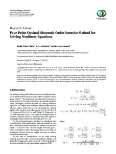
6. Basins of Attraction To study the dynamical behavior, we generate basins of attraction for two different polynomials using the above-mentioned methods. Following [29], we take a square [−1, 1] × [−1, 1]

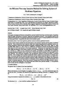
(⊆ C) of 1024 × 1024 points, which contains all roots of concerned nonlinear equation, and we apply the iterative method starting in every 𝑧0 in the square. We assign a color to each point 𝑧0 according to the simple root to which the corresponding orbit of the iterative method, starting from 𝑧0 , converges. If the corresponding orbit does not reach any root of the polynomial, with tolerance 𝜖 = 10−3 in a maximum of 25 iterations, we mark those points 𝑧0 with black color. For the first test problem 𝑝1 (𝑧) = 𝑧2 − 1, Figure 1 clearly shows that the proposed method SBM (Figure 1(f)) seems to produce larger basins of attraction than CLM (Figure 1(e)) and CM (Figure 1(d)), almost competitive basins of attraction as KLM (Figure 1(c)), and smaller basins of attraction than NM (Figure 1(a)) and KM (Figure 1(b)). In our next problem, we have taken the cubic polynomial 𝑝2 (𝑧) = 𝑧3 − 1. The results are given in Figure 2. Again the proposed method SBM (Figure 2(f)) seems to produce larger basins of attraction than KM (Figure 2(b)), CM (Figure 2(d)), and CLM (Figure 2(e)), almost competitive basins of attraction as KLM (Figure 2(c)), and smaller basins of attraction than NM (Figure 2(a)).

7. Conclusion In this work, we have proposed an optimal method of fourth order for finding simple roots of nonlinear equations. The advantage of the proposed method is that it does not require the use of second order derivative. The numerical results have confirmed the robustness and efficiency of the proposed method. The presented basins of attraction also show the good performance of the proposed method as compared to other existing fourth order methods in the literature.

Conflict of Interests The authors declare that there is no conflict of interests regarding the publication of this paper.

Acknowledgment One of the authors acknowledges I. K. Gujral Punjab Technical University, Kapurthala, Punjab, for providing research support to her.

References [1] J. M. Ortega and W. C. Rheinboldt, Iterative Solution of Nonlinear Equations in Several Variables, Academic Press, New York, NY, USA, 1970. [2] S. C. Chapra and R. P. Canale, Numerical Methods for Engineers, McGraw-Hill, New York, NY, USA, 1988. [3] J. F. Traub, Iterative Methods for the Solution of Equations, Chelsea Publishing Company, New York, NY, USA, 1977. [4] M. S. Petković, B. Neta, L. D. Petković, and J. Dzunić, Multipoint Methods for Solving Nonlinear Equations, Academic Press, 2013. [5] A. M. Ostrowski, Solution of Equations and Systems of Equations, Academic Press, New York, NY, USA, 1960. [6] B. Neta, Numerical Methods for the Solution of Equations, NetA-Sof, Monterey, Calif, USA, 1983.

Journal of Complex Analysis [7] S. Weerakoon and T. G. I. Fernando, “A variant of Newton’s method with accelerated third order convergence,” Applied Mathematics Letters, vol. 13, no. 8, pp. 87–93, 2000. [8] E. Halley, “A new and general method of finding the roots of equations,” Philosophical Transactions of the Royal Society of London, vol. 18, pp. 136–138, 1694. [9] E. Hansen and M. Patrick, “A family of root finding methods,” Numerische Mathematik, vol. 27, no. 3, pp. 257–269, 1977. [10] R. F. King, “A family of fourth order methods for nonlinear equations,” SIAM Journal on Numerical Analysis, vol. 10, no. 5, pp. 876–879, 1973. [11] C. Chun, “A family of composite fourth-order iterative methods for solving nonlinear equations,” Applied Mathematics and Computation, vol. 187, no. 2, pp. 951–956, 2007. [12] C. Chun and Y. Ham, “A one-parameter fourth-order family of iterative methods for nonlinear equations,” Applied Mathematics and Computation, vol. 189, no. 1, pp. 610–614, 2007. [13] C. Chun, M. Y. Lee, B. Neta, and J. Dˇzunić, “On optimal fourthorder iterative methods free from second derivative and their dynamics,” Applied Mathematics and Computation, vol. 218, no. 11, pp. 6427–6438, 2012. [14] A. Cordero, J. L. Hueso, E. Mart´ınez, and J. R. Torregrosa, “New modifications of Potra-Pták’s method with optimal fourth and eighth orders of convergence,” Journal of Computational and Applied Mathematics, vol. 234, no. 10, pp. 2969–2976, 2010. [15] J. Kou, X. Wang, and Y. Li, “Some eighth-order root-finding three-step methods,” Communications in Nonlinear Science and Numerical Simulation, vol. 15, no. 3, pp. 536–544, 2010. [16] J. Kou, Y. Li, and X. Wang, “A composite fourth-order iterative method for solving non-linear equations,” Applied Mathematics and Computation, vol. 184, no. 2, pp. 471–475, 2007. [17] P. Jarratt, “Some fourth order multipoint methods for solving equations,” Mathematics of Computation, vol. 20, pp. 434–437, 1966. [18] J. H. Curry, L. Garnett, and D. Sullivan, “On the iteration of a rational function: computer experiments with Newton’s method,” Communications in Mathematical Physics, vol. 91, no. 2, pp. 267–277, 1983. [19] E. R. Vrscay, “Julia sets and mandelbrot-like sets associated with higher order Schröder rational iteration functions: a computer assisted study,” Mathematics of Computation, vol. 46, no. 173, pp. 151–169, 1986. [20] E. R. Vrscay and W. J. Gilbert, “Extraneous fixed points, basin boundaries and chaotic dynamics for Schröder and König rational iteration functions,” Numerische Mathematik, vol. 52, no. 1, pp. 1–16, 1987. [21] S. Amat, S. Busquier, and S. Plaza, “Review of some iterative root-finding methods from a dynamical point of view,” Scientia, Series A, vol. 10, pp. 3–35, 2004. [22] S. Amat, S. Busquier, and S. Plaza, “Dynamics of the king and jarratt iterations,” Aequationes Mathematicae, vol. 69, no. 3, pp. 212–223, 2005. [23] P. Blanchard, “The dynamics of Newton’s method,” Proceedings of Symposia in Applied Mathematics, vol. 49, pp. 139–154, 1994. [24] F. Chicharro, A. Cordero, J. M. Gutiérrez, and J. R. Torregrosa, “Complex dynamics of derivative-free methods for nonlinear equations,” Applied Mathematics and Computation, vol. 219, no. 12, pp. 7023–7035, 2013. [25] B. Neta, C. Chun, and M. Scott, “Basins of attraction for optimal eighth order methods to find simple roots of nonlinear equations,” Applied Mathematics and Computation, vol. 227, pp. 567–592, 2014.

9 [26] D. K. R. Babajee, A. Cordero, F. Soleymani, and J. R. Torregrosa, “On improved three-step schemes with high efficiency index and their dynamics,” Numerical Algorithms, vol. 65, no. 1, pp. 153–169, 2014. [27] W. Gautschi, Numerical Analysis: An Introduction, Birkhaüser, Boston, Mass, USA, 1997. [28] S. Wolfram, The Mathematica Book, Wolfram Media, 5th edition, 2003. [29] J. L. Varona, “Graphic and numerical comparison between iterative methods,” The Mathematical Intelligencer, vol. 24, no. 1, pp. 37–46, 2002.

Advances in

Operations Research Hindawi Publishing Corporation http://www.hindawi.com

Volume 2014

Advances in

Decision Sciences Hindawi Publishing Corporation http://www.hindawi.com

Volume 2014

Journal of

Applied Mathematics

Algebra

Hindawi Publishing Corporation http://www.hindawi.com


Volume 2014

Journal of

Probability and Statistics Volume 2014

The Scientific World Journal Hindawi Publishing Corporation http://www.hindawi.com


Volume 2014

International Journal of

Differential Equations Hindawi Publishing Corporation http://www.hindawi.com

Volume 2014

Volume 2014

Submit your manuscripts at http://www.hindawi.com International Journal of

Advances in

Combinatorics Hindawi Publishing Corporation http://www.hindawi.com

Mathematical Physics Hindawi Publishing Corporation http://www.hindawi.com

Volume 2014

Journal of

Complex Analysis Hindawi Publishing Corporation http://www.hindawi.com

Volume 2014

International Journal of Mathematics and Mathematical Sciences

Mathematical Problems in Engineering

Journal of

Mathematics Hindawi Publishing Corporation http://www.hindawi.com

Volume 2014


Volume 2014

Volume 2014


Volume 2014

Discrete Mathematics

Journal of

Volume 2014


Discrete Dynamics in Nature and Society

Journal of

Function Spaces Hindawi Publishing Corporation http://www.hindawi.com

Abstract and Applied Analysis

Volume 2014


Volume 2014


Volume 2014

International Journal of

Journal of

Stochastic Analysis

Optimization



Volume 2014

Volume 2014