Contents
Page 1 of 14
Print
An Optimal Spatial Sampling Scheme to Characterize Mine Tailings Pravesh Debba1; Emmanuel John M. Carranza2; Alfred Stein2; Freek D. van der Meer2 CSIR, Built Environment, Logisitics and Quantitative Methods, PO Box 395, Pretoria, 0001, South Africa. 2 International Institute for Geo-Information Science and Earth Observation (ITC), Hengelosestraat 99, PO Box 6, 7500 AA, Enschede, The Netherlands. E-mail:
[email protected];
[email protected];
[email protected];
[email protected]
Sessions
STCPMs
1
T
INTRODUCTION Geochemical characterization of mine waste impoundments is important for rehabilitation, or for remediation, to protect the surrounding environment and ecosystems. For effective geochemical characterization, this would entail surface (to subsurface) sampling, which could be labor or cost intensive, especially if not properly planned. Metals in mine waste impoundments are usually hosted by acid-generating sulphide-rich minerals, for e.g., pyrite, pyrrhotite, or adsorbed onto surfaces of weathering products of such sulphide-rich minerals. Unfortunately, such minerals are difficult to detect or identify by using current remote sensing techniques including multispectral or even hyperspectral data. It has been shown, however, that certain sulphide-rich minerals, particularly pyrite, weathers to a series of iron-bearing sulfates, hydroxides and oxides (Swayze et al., 2000). Such secondary ironbearing sulfates/hydroxides/oxides have diagnostic spectral features (Crowley et al., 2003), which enable their detection or identification with analytical techniques using hyperspectral data.
Contents
Page 2 of 14
Sessions
STCPMs
Print
Debba et al. (2006) demonstrated the potential of using hyperspectral data to estimate abundances of spectrally similar iron-bearing sulfates/hydroxides/oxides. It has also been shown that heavy metal contamination in soils can be quantified using reflectance spectroscopy (Kemper & Sommer, 2002). Thus, remote sensing technology potentially provides an indirect tool for surface characterization of mine waste impoundments with oxidizing sulphide-rich materials; namely, for mapping spatial distributions of secondary iron-bearing sulfates/hydroxides/oxides and thereby modeling the spatial distribution of heavy metals. Hence given a model of spatial distribution of secondary iron-bearing oxides/hydroxides, the problem is how to design a sampling scheme that would adequately capture the spatial distribution of certain groups of metals. In a recent paper, Diggle & Lophaven (2006) discuss a retrospective sampling design, which sequentially removes, from a sampling design, samples that contribute least to a Bayesian prediction of a response. They do, however, state that this is not the optimal design. In this paper, a prospective sampling scheme is derived for nearby unsampled areas based on the variogram model of the adjacent sampled area. The present case study area is in the Recsk-Lah´oca copper mining area in Hungary. STUDY AREA The Recsk-Lah´oca mining area is situated in the M´atra Mountains, about 110 km northeast of Budapest, Hungary. Mining of ore deposits in the Recsk-Lah´oca area resulted in the exposure of sulphide bearing-rocks to surface water and atmospheric oxygen, which accelerate oxidation, leaching and release of metals and acidity. Mine tailings and waste rock dumps resulting from the two-century mining of copper and gold are present in the area.
T
Contents
Page 3 of 14
Print
Sessions
STCPMs
DATA
T
In this study, a subset of the Digital Airborne Imaging Spectrometer (DAIS-7915) is used. The resulting data is a 79 channel hyperspectral image, acquired over Recsk. The hyperspectral image taken on 18th August 2002 is shown in Figure 1 at 5 m nominal resolution on the ground. Not all 79 channels were useful as many channels were too noisy and could not be corrected efficiently. Fortunately, the first 32 channels, spectral range 406-1035 nm, where iron-bearing oxides/hydroxides/sulphates have diagnostic features were found useful for this study. Fig. 1: The “East Tails” and the “West Tails” shown in a color composite image of the DAIS data. Ratios of ch17 to ch28 (representing ferrihydrite reflectance and absorption peaks) was used as red band, ch13 to ch25 (representing jarosite reflectance and absorption peaks) was used as green band and ch32 to ch1 (representing non-iron-bearing minerals) was used as blue band. Red dots are locations of mine tailings samples. Short dashed lines indicates drainage lines of either active or non-active streams. Samples from the tailings (Figure 1) were collected a few minutes shortly after collection of the DAIS hyperspectral data. Fifty-three samples were collected in the East Tails and 44 in the West
Contents
Page 4 of 14
Print
tails. Samples of tailings were collected at 10m×10m grid points in portions of the tailings dumps with almost no vegetation cover within 3 m radius. Portions of the tailings dumps, close to the active stream have steep slopes and were not sampled. Samples were collected from the top surface of the tailings and were analyzed in the laboratory. Concentrations of As, Cd, Cu, Fe, Mn, Ni, Pb, Sb and Zn in the decomposed samples were determined using the ICP-AES analyzer.
Sessions
STCPMs
METHODS The East Tails and the West Tails have different geochemical characteristics, hence it was decided to split the data into two sets. The small stream between the East Tails and the West Tails provides a natural boundary to do so. Data from either sub-area are used to model a relationship between heavy metal associations and relative abundances of secondary iron-bearing minerals. The latter data are derived from spectral unmixing of hyperspectral data. A model relationship between heavy metal associations and mineral abundances in one sub-area is then used as basis for optimal sampling design in the other sub-area. Division of the area and the data thus provides calibration analysis and prediction/validation analysis for optimal sampling design. Estimation of mineral abundance
T
Spectral unmixing of hyperspectral data was performed to estimate relative abundance or proportion, per 5 m pixel, of secondary iron-bearing minerals, with which metals in the mine tailings could be associated. Spectral unmixing is a deconvolution process for estimating proportional contributions of each end-member to spectra. Debba et al. (2006) suggested that better abundance estimates are
Contents
Page 5 of 14
Sessions
STCPMs
Print
obtained if materials, not necessarily of interest but are probably present, and contribute to a pixel spectrum is also included in an end-member set for spectral unmixing. Accordingly, copiapite, jarosite, goethite, ferrihydrite, hematite, kaolinite, anhydrite, gypsum, quartz, and tumbleweed (grass) was considered to consist the end-member set. Abundance estimates were determined according to the method of Debba et al. (2006), which involves minimization of variance of the differences between the first derivative of an estimated spectrum and the first derivative of an actual spectrum after smoothing the spectra. It was found that copiapite is least abundant and hematite is highly abundant in the mine tailings dumps. Modeling of heavy metal associations Concentrations of several metals in soils can be estimated using reflectance spectroscopy (Kemper & Sommer, 2002). In addition, geochemical sampling addresses a suite of metals, which reflect intrinsic processes in a system, like a mine tailings dump. It was thus decided to model a heavy metals association reflecting scavenging of metals by secondary iron-bearing minerals in the mine tailings dumps. A factor component analysis with varimax rotation was performed on the logarithmictransformed heavy metal concentrations to obtain the heavy metal association of interest. The scores of FA2E and FA2W are then linearly transformed to [0, 1], for numerical compatibility with the mineral abundance estimates, and labeled FA2ET and FA2WT, respectively. Kriging with external drift
T
Kriging with external drift is applicable to estimate primary variables of interest, which are
Contents
Page 6 of 14
Sessions
STCPMs
Print
practically measurable at only few sample sites, based on linearly related ancillary variables, which are measurable at much higher sampling density than the primary variables. Wackernagel (1998) suggests that such ancillary variables can be incorporated into a kriging system as external drift functions. Kriging with external drift is ideal if a primary variable could be measured more precisely and practically at a few locations, whereas possibly less accurate measurements of linearly related ancillary variables are available everywhere in the spatial domain. The present case study applies kriging with external drift to model a relationship between heavy metal association of interest and metal-savenging minerals in the mine tailings dumps. The distribution of heavy metal associations, represented as factor scores, were used as the primary variable of interest and is based on field sampling. The relative abundances of metal-scavenging iron-bearing minerals, which were obtained from hyperspectral data, are the ancillary variables. For the modeling, consider x ∈ A ⊂ R2 to be a generic data location (xu , xv ) in 2-dimensional Euclidean space and suppose the domain Z(x) at spatial location x is a random quantity. The multivariate random field {Z(x) : x ∈ A}, is generated by letting x vary over index set A ⊂ R2 . A realization of of this is denoted {z(x) : x ∈ A}. The variogram is defined as the average squared difference between values separated by a given lag h, where h is a vector in both distance and direction, that is, (1)
2γ(h) = E[Z(x) − Z(x + h)]2 .
Hence the semi-variogram γ(h) is defined as: (2)
T
1 γ(h) = E[Z(x) − Z(x + h)]2 . 2
Page 7 of 14
Contents Print
The experimental semi-variogram γ ? (h) may be obtained from κ = 1, 2, . . . , P (h) pairs of observations {z(xκ ), z(xκ + h)} at locations {xκ , xκ + h}, as: (3)
P (h) X 1 [z(xκ ) − z(xκ + h)]2 . γ (h) = 2 · P (h) ?
Sessions
STCPMs
κ=1
Suppose that precise measurements are available for a primary variable Z(x) with nB observations, which is assumed to be a second order random function with known covariance function C(h), hence the variogram γ(h) = C(h)/C(0) is assumed to be known. The k ancillary variables represented as regionalized variables yi (x), i = 1, . . . , k with nA observations, are less accurate measurements covering the whole domain A at small scale and are considered as deterministic. The values {yi (x)} needs to be known at all locations xα of the samples as well as at the nodes of the estimation grid. Since Z(x) and the set of {yi (x)} are two ways of expressing the same phenomenon, assume that Z(x) is an average equal to a linear function of the set of {yi (x)} up to a constant b0 and coefficients bi , i = 1, . . . , k, (4)
E[Z(x)] = b0 +
k X i=1
T
bi · yi (x) =
k X
bi · yi (x) ,
i=0
where y0 (x) = 1. The method of merging both sources of information uses {yi (x)} as an external drift function for the estimation of Z(x). The drift of Z(x) is defined externally through the ancillary variables {yi (x)} rather than some smooth version of Z(x) itself, (Chil`es & Delfiner, 1999). Assuming Z(x) is a second order stationary random function, then
Page 8 of 14
Contents Print
(5)
∗
Z (x0 ) =
nA X
λα Z(xα )
α=1
where λα denotes the weight of the αth observation and is constraint to unit sum. In estimating the external drift coefficients, the following conditions,
Sessions
STCPMs
(6)
nA X
λα yi (xα ) = yi (x0 ) ,
i = 1, . . . , k ,
α=1
are added to the kriging system independently of the inference of the covariance function, hence the term “external”. The kriging variance can then be written as (7)
2 σKED (x0 ) = Var[Z(x0 ) − Z ∗ (x0 )] .
The only factor influencing the kriging variance are the variogram γ(h), the number of observations nA , the sampling locations xα and the location x0 . This means that the kriging variance does not depend on the observations themselves, but rather only on their relative spacing. The advantage is that in can be used to optimize sampling schemes in advance of data collection. In this paper, the location and the covariates as external drift were used to estimate the heavy metal concentration, E[Z(x)] = b0 + b1 · xu + b2 · xv + b3 · GOE(x) + b4 · JAR(x) + b5 · FER(x) + b6 · HEM(x) (8)
T
+b7 · KAO(x) + b8 · COP(x) ,
Contents
Page 9 of 14
Print
namely, a first order polynomial on the coordinates and the abundance estimates of the metalscavenging minerals. In Equation 8, GOE is abundance estimates for goethite, JAR is for jarosite, FER is for ferrihydrite, HEM is for hematite, KAO is for kaolinite, and COP is for copiapite.
Sessions
STCPMs
Sampling scheme optimization
T
For a two-dimensional area A, let the collection of all possible sampling schemes with n observations on A be denoted by Sn . A fitness function φ(Sn ) : Sn → R+ is minimized through simulated annealing. In terms of sampling, the initial step in simulated annealing is to randomly select a set of points in A. A new point in A is then randomly selected and replaces a randomly selected old point from the current collection. This replacement occurs, based on a probabilistic criterion, if the fitness function decreases and if the fitness function increases. Hence, the process allows inferior moves. Initially, the probabilistic criterion is high, allowing a large probability of inferior moves. A parameter in the annealing process is then reduced by a factor of 0.95 at each successive step, thereby decreasing the probability of accepting inferior moves until the process stabilizes. The final solution is independent of the initial random selection of points as the process reaches the global optimum. A variogram model for a previously sampled area can be used to estimate σ 2 (x) (Equation 7) in an unvisited area, if the latter is considered to have similar, if not the same, spatial characteristics as the former. In this case, estimates of σ 2 (x) in the unvisited area can be used to derive the optimal prospective sampling scheme. The optimization procedure by simulated annealing is then performed by application of a criterion called the Mean Kriging Variance with External Drift (MKVED), the fitness function of which is defined as
Contents
Page 10 of 14
Print
(9)
nA 1 X 2 σKED (xA,j |S) , φMKVED (S) = nA
Sessions
STCPMs
j=1
T
where nA is the number of raster nodes for which data for each of the covariates are available. The MKVED-criterion is ideal for deriving optimal prospective sampling schemes, since it does not depend on the actual data for the primary variable. It depends, however, on a covariance function, the spatial configuration of sampling locations and data locations of the covariates (Equation 7). Hence, the MKVED-criterion is proposed to derive the optimal prospective sampling scheme in an unvisited area based on a relevant model from a previously sampled area. RESULTS: OPTIMAL PROSPECTIVE SAMPLING SCHEMES By way of simulated annealing, a prospective sampling scheme for the West Tails is derived based on a model for the East Tails. As an illustration, it was decided to derive a prospective sampling scheme having 30 samples in the West Tails using the 53 samples from the East Tails. The exponential variogram was estimated with the data from the East Tails and is shown in Figure 2(a). To verify that this variogram is also appropriate for the West Tails, the East and West Tails data were combined and the variogram is shown in Figure 2(b). The similarity of the two variograms indicate that the variogram for the East Tails could be appropriate for modeling the West Tails.
Page 11 of 14
Contents Print
Sessions
STCPMs
Fig. 2: The exponential variogram for the East Tails, combined East & West Tails and prospective optimal sampling scheme in the West Tails using East Tails samples.
T
(a) East Tails
(b) East and West Tails combined
(c) Prospective sampling scheme
Variogram model for the East Tails was applied to the West Tails data to derive a prospective sampling scheme via simulated annealing to minimize Equation 9. The resulting prospective sampling scheme, with 30 samples for the West Tails, is shown in Figure 2(c). The optimal sampling scheme constructed using the kriging external drift variance approach are spread over the West Tails region while retaining some close pairs of samples. These close pair samples are to improve the estimation of the variogram model. The mean kriging with external drift variance for the West Tails, using the combined East and West Tails sampling data, as illustrated in Figure 1, is 6.8 × 10⁻⁴ for the West Tails. This mean kriging variance was approximately the same when either of the two variograms was used. The
Contents
Page 12 of 14
Print
optimal sampling scheme resulted in a mean kriging with external drift variance for the West Tails of 3.3 × 10⁻⁴ using the variogram derived from the East Tails data. This indicates that the optimal sampling scheme contains samples that reduces the mean kriging with external drift variance for the previously designed grid sampling scheme in the West Tails.
Sessions
STCPMs
DISCUSSION AND CONCLUSIONS
T
Surface characterization of mine tailings could provide essential information for protection of surrounding ecosystems. Planning where tailings samples should be collected is therefore a crucial task. This is so because spatial distributions of undesirable heavy metals in mine tailings must be determined accurately. This study has demonstrated usefulness of airborne hyperspectral data to support optimization of sampling schemes for surface characterization of mine tailings. Analysis of hyperspectral data can yield information about spatial distributions of secondary iron-bearing and clay minerals associated with weathering of pyrite-rich mine wastes. Heavy metals usually reside in such secondary minerals. Nevertheless, field samples are necessary to model spatial relationships between heavy metals and secondary minerals in mine tailings. The data collected in an orientation grid sampling program must allow determination of (a) spatial distributions of heavy metals, (b) spatial distributions of secondary metal-scavenging minerals, (c) spatial relationships between heavy metals and secondary metal-scavenging minerals, and (d) a variogram model of heavy metal associations due to metal-scavenging minerals. These four types of spatial information are essential to optimize a prospective sampling scheme to be carried out during a main sampling program, especially for large mine tailings.
Contents
Page 13 of 14
Sessions
STCPMs
Print
This study has shown that spatial relationships between heavy metals and metal-scavenging minerals can be modeled adequately by kriging with external drift. The kriging variance, being dependent only on the variogram, the spatial configuration of the sampling locations and the data locations, could then be used to derive optimal sampling schemes. In conclusion, the use of secondary information in designing optimal sampling schemes was also illustrated. Often these secondary information can be achieved at a relatively low cost and available over a greater region. These are the primary reasons for incorporating this information into the sampling design. Optimized sampling schemes using the mean kriging with external drift variance will result in sampling schemes that explicitly take into account the nature of spatial dependency of the data and together with hyperspectral data can be used to design sampling schemes in nearby unexplored areas.
References Chil`es, J.-P. & Delfiner, P. (1999). Geostatistics: Modeling spatial uncertainty. John Wiley & sons, INC. Crowley, J. K., Williams, D. E., Hammarstrom, J. M., Piatak, N., Chou, I. M., & Mars, J. C. (2003). Spectral reflectance properties (0.4–2.5 µm) of secondary Fe-oxide, Fe-hydroxide, and Fe-sulphatehydrate minerals associated with sulphide-bearing mine wastes. Geochemistry: Exploration, Environment, Analysis, 3(2), 219–228.
T
Contents
Page 14 of 14
Print
Debba, P., Carranza, E. J. M., van der Meer, F. D., & Stein, A. (2006). Abundance estimation of spectrally similar materials by using derivatives in simulated annealing. IEEE Geoscience and Remote Sensing, (12), 3649–3658.
Sessions
STCPMs
Diggle, P. & Lophaven, S. (2006). Bayesian geostatistical design. Scandinavian Journal of Statistics, 33, 53–64.
T
Kemper, T. & Sommer, S. (2002). Estimate of heavy metal contamination in soils after a mining accident using reflectance spectroscopy. Environmental Science and Technology, 36(12), 2742–2747. Swayze, G. A., Smith, K. S., Clark, R. N., Sutley, S. J., Pearson, R. M., Vance, J. S., Hageman, P. L., Briggs, P. H., Meier, A. L., Singleton, M. J., & Roth, S. (2000). Using imaging spectroscopy to map acidic mine waste. Environmental Science and Technology, 34, 47–54. Wackernagel, H. (1998). Multivariate Geostatistics: An Introduction with Applications. SpringerVerlag Germany, second edition.