An Optimization Approach for Automated Unit Test ...

Accepted Manuscript An Optimization Approach for Automated Unit Test Generation Tools using Multiobjective Evolutionary Algorithms Samar Ali Abdallah, Ramadan Moawad, Esaam Eldeen Fawzy PII:

S2314-7288(18)30007-2

DOI:

10.1016/j.fcij.2018.02.004

Reference:

FCIJ 38

To appear in:

Future Computing and Informatics Journal

Received Date: 16 January 2018 Revised Date:

7 February 2018

Accepted Date: 19 February 2018

Please cite this article as: Abdallah SA, Moawad R, Fawzy EE, An Optimization Approach for Automated Unit Test Generation Tools using Multi-objective Evolutionary Algorithms, Future Computing and Informatics Journal (2018), doi: 10.1016/j.fcij.2018.02.004. This is a PDF file of an unedited manuscript that has been accepted for publication. As a service to our customers we are providing this early version of the manuscript. The manuscript will undergo copyediting, typesetting, and review of the resulting proof before it is published in its final form. Please note that during the production process errors may be discovered which could affect the content, and all legal disclaimers that apply to the journal pertain.

ACCEPTED MANUSCRIPT

An Optimization Approach for Automated Unit Test Generation Tools using Multi-objective Evolutionary Algorithms Ramadan Moawad

Esaam Eldeen Fawzy Chairman of Computer Science Dep. Arab Academy of Science, Technology & Maritime Transport Cairo, Egypt [email protected]

AC C

EP

TE D

M AN U

SC

Vice-Dean of Collage of Computer and Information Technology Future University in Egypt Cairo, Egypt [email protected]

RI PT

Samar Ali Abdallah Faculty of Computing and Information Technology Arab Academy for Science, Technology & Maritime Transport Cairo, Egypt [email protected]

ACCEPTED MANUSCRIPT

Keywords—Unit Test; Automated test case generation; MOEA; Code Coverage.

I.

INTRODUCTION

SC

MOEA is a significant topic that requires careful heed when addressing real-world problems. Most real-world MOPs (Multi-Objective Problems) have constraints that need to be incorporated into our search engine to avoid convergence towards infeasible solutions. Constraints can be “hard” (i.e., they must be satisfied) or “soft” (i.e., they can be relaxed), and addressing them properly has been a matter of research within single-objective EAs. [4] [2] MOEA is particularly effective at finding solutions to elusive problems while another MOEA is effective at solving non-uniform Pareto fronts. If one does not know the phenotype space of the problem, using multiple MOEAs with distinctive strengths may prove better than using just one. The MOEAs could then coevolve in such a way that individuals pass from one algorithm to another in an attempt to seed the algorithms with good solutions. [2]

M AN U

Abstract—High code coverage is measured by the process of software testing typically using automatic test case generation tools. This standard approach is usually used for unit testing to improve software reliability. Most automated test case generation tools focused just on code coverage without considering its cost and redundancy between generated test cases. To obtain optimized high code coverage and to ensure minimum cost and redundancy a Multi-Objectives Evolutionary Algorithm approach (MOEA) is set in motion. An efficient approach is proposed and applied to different algorithms from MOEA Frame from the separate library with three fitness functions for Coverage, Cost, and Redundancy. Four MEOA algorithms have been proven reliable to reach above the 90 percent code coverage: NSGAII, Random, SMSEMOA, and ϵ-MOEA. These four algorithms are the key factors behind the MOEA approach.

RI PT

An Optimization Approach for Automated Unit Test Generation Tools using Multi-objective Evolutionary Algorithms

EP

TE D

"Software testing is used as a procedure to ensure that the programs are free from bugs and to improve their function performance. In other words, it is used to determine and improve the quality of the software". Before starting the testing process, it is necessary to choose a test adequacy criterion to evaluate whether a suite is adequate concerning the test goals [1]. A test adequacy criterion defines properties that must be observed by the test suite (e.g., code coverage, functional requirements’ coverage, among others).

AC C

Code coverage [10] is considered a way to guarantee that tests are testing the code. When testers run those tests, they are presumably checking that the expected results obtained. Coverage measurement is useful in many ways; it improves the testing process, gives the information to the user about the status of the verification process, and helps to find areas that are not covered. Several tools are ranging from manual and automated generation test cases to facilitate the software testing process. The future lies in the automated approach to generate test cases; however, it is prone to errors and is time-consuming. This entails a rise in the cost of the testing process. We introduce, in our research paper, a new approach to optimize the test cases generation process to decrease the cost of running the unit tests. This process eliminates redundancies; thus, it increases efficiency. As a result, code coverage is maximized. We have incorporated four MEOA algorithms.

In our research paper, we select four different algorithms: NSGAII, Random, SMSEMOA, and ϵ-MOEA from different libraries with different behavior to provide efficient solutions. The paper is organized as follows. The next section, some of the related work to our research. In Section 3, we propose the approach to select test cases for automated test cases Generation tools. In Section 4, the different used datasets are presented. In section 5 the brief different algorithms are used in our research. Finally, the experiments and results are discussed in section 6. II.

RELATED WORK

Luciano S. de Souza, Pericles B. C. de Miranda, Ricardo B. C. Prudencio and Flavia de A. Barros presented in [4] a method that uses Particle Swarm Optimization (PSO) to solve multiobjective Test Case selection problems. In contrast to singleobjective difficulties, Multi-Objective Optimization (MOO) optimize more than one objective at the same time. They developed a mechanism for functional Test Case selection which considers two objectives simultaneously: maximize code coverage while minimizing cost in of Test Case execution effort based on Particle Swarm Optimization (PSO). They implement two multi-objective versions of PSO (BMOPSO and BMOPSO-CDR). During this work developed a Binary Multi-Objective PSO (BMOPSO), as the solutions of the TC selection problem which represented as binary vectors; and (2) the MOPSO algorithm to work with multi-objective problems. Also, implemented the BMOPSO-CDR algorithm by adding

TE D

M AN U

SC

RI PT

ACCEPTED the Crowding Distance and Roulette Wheel mechanism to the MANUSCRIPT In the testing process, it is necessary to choose a test BMOPSO to select functional tests. adequacy criterion defines properties that must be observed by the test suit. The most important metrics we must concern Luciano S. de Souza, Pericles B. C. de Miranda, Ricardo B. about it is the critical objective which is Code Coverage and C. Prudencio and Flavia de A. Barros presented enhancement the constraints which are the cost of execution time and to previous work in [5] added the so-called catfish effect into redundancy between generated test cases. The cost and the multi-objective selection algorithms to enhance their redundancy are the critical constraints to cut down these suits, results. The use of the so-called “catfish” effect, for instance, to fit the available resources, without severely settling the has shown to improve the performance of the single objective coverage of the test fitness criterion signifying recognized. version of the binary PSO. The catfish effect derives its name Reduce the generated test suite based on some selection from an effect that Norwegian fishermen observed when they criterion is known as "Test Case Selection" process. introduced catfish into a holding tank for caught sardines. The introduction of a catfish, which is different from sardines, into A. Proposed Structure the tank resulted in the stimulation of sardine movement, so Our approach as in fig 1 we use two different datasets of keeping the sardines alive and therefore fresh for a longer time. test suits which have a different number of test cases to cover Similarly, the catfish effect was developed to the PSO the same program and the number of requirements. Each test algorithm in such way that we introduce “catfish particles” to suit has different behavior in the total cost and redundancy stimulate a renewed search by the rest of the swarm’s particles. between test cases. We develop encoder by java programming Hence, these catfish particles help to guide the particles, which language to encode the different metrics in each dataset can be trapped in a local optimum, to new regions of the search (coverage, cost, and redundancy) for each test case. As said, space and thus leading to possible better areas. three fitness functions were adopted. The requirements Chandraprakash Patidar presented in [6] approach for test coverage objective (to be maximized) represents the amount (in case generation algorithms using Sequence Diagram Based percentage) of requirements covered by a solution d in Testing with discrete particle swarm optimization algorithm. comparison to the number of requirements present in D which The approach presented automated test case generation from is the selected test case from the dataset. Formally, let X = {X1, UML sequence diagram using discrete Particle Swarm …, Xr} be a given set of X requirements of the original suite Optimization Algorithm. In his approach introduced an D. Let F(Dj) be a function that returns the subset of algorithm that automatically creates a dependency then it requirements in X covered by the individual test case: Dj for generated a dependency graph from which test cases can each one. generated test cases. Also, generating dynamic test cases by using sequence diagram as a base element for generating test Then, the requirements coverage of a solution d as given: cases using sequence diagram dynamic actions like interaction among objects can be taken into consideration when generating Coverage(d) = 100 * Unit: (%) test cases. Finally, present optimization using discrete particle swarm optimization algorithm. Apply on the test cases The Cost fitness function calculated as the summation of run generated by dependency graph generated by extracted time in milliseconds of each test cases selected in provided information from sequence diagram. solution d from dataset D as given:

AC C

EP

III. PROPOSED APPROACH In this paper, we proposed a new approach that adopts four different algorithms and three fitness functions to solve multiobjective test cases selection problems in many automated test cases generation tools. Which is facing the challenge of generating duplicated test cases and ineffective within the cost of execution time furthermore give lower coverage percentage also the redundancy among test cases. Where customers search for high-quality products, the software testing activity has grown in importance, aiming to assure quality and reliability to the product under development. Also generating a massive number of test cases is costly, reaching up to 40% of final software development cost. Thus, it is of central importance to improve the efficiency and effectiveness of the whole testing process.

Cost(d) =

Unit: (ms)

Redundancy fitness function which is more complicated because of redundancy indicator that retrieves the test cases with redundant coverage of requirements. The fitness function is the total number of redundant test cases divided by the total number of test cases selected in provided solution d. Red(d) =

Unit: (%)

After that, the evaluation functions run with the multiobjective algorithms to find an efficient Preto front regarding the fitness functions Coverage, Cost, and Red.

M AN U

SC

RI PT

ACCEPTED MANUSCRIPT

Fig 1. Proposed Approach

B. Proposed Preprocesses

EP

TE D

In this section, we will provide our standard tuning to all selected algorithms that are running the above fitness functions on our two datasets. Each algorithm has parameters include the population size, the simulated binary crossover (SBX) rate and distribution index, and the polynomial mutation (PM) rate and distribution index and Max Evaluations. We are tuning each algorithm by the same value to all parameters So that we can measure the efficiency of each algorithm. The tuning parameters values as following: 1) populationSize = 1000 2) sbx.rate = 0.9

3) sbx.distributionIndex = 15.0

5)

AC C

4) pm.rate = 0.1

pm.distributionIndex = 20.0

6) MaxEvaluations = 1000 IV.

Data selection

We have two different datasets for implemented program with 745 line of code which is mean we have 745 requirements to covered by our datasets of test cases. The first dataset has 83 test cases with total code coverage 100% and total run time cost 337.6 milliseconds, and total redundancy 40 between test cases. The second dataset have 70 test cases with total code 100% and total run time cost 299.9 milliseconds,

and total redundancy 25 between test cases. We select that two datasets to prove our concept of select efficient test cases with high code coverage and minimum cost and redundancy. V.

Algorithms selection

Our selected algorithms are implemented within the MOEA Framework and thus support all functionality provided by the MOEA. The four algorithms selected from two different library Native Algorithms and JMetal Algorithms. The NSGAII, ϵ-MOEA and Random Search are from Native Algorithms library. SMSEMOA from JMetal Algorithms library. Each algorithm of them has different behavior to generate many solutions. We will provide a brief about each of them as follows: A. ϵ-MOEA ϵ-MOEA is a steady-state MOEA that uses ϵ-dominance archiving to record a diverse set of Pareto optimal solutions [7]. ϵ-MOEA algorithm the search space is divided into a number of hyper-boxes or grid and the diversity is maintained by ensuring that a hyper-box occupied by only one solution. There are two co-evolving populations: (i) an EA population P(t) and (ii) an archive population E(t) where t is the iteration counter. The archive population stores the nondominated solutions and is updated iteratively with the e-dominance concept. Moreover, the EA population is updated iteratively with the usual domination. [8]

VI.

Results and Analysis

AC C

EP

TE D

Multiple experiments are performed to improve code coverage and reduce the cost and redundancy of the selected program that has 745 lines of code for each dataset. Our primary objective to maximize the coverage of 745 line of code we have with a concern about the runtime cost of running the test cases of each dataset we have. In this section, we will present the results of our experiments for each dataset running with the selected four algorithms (ϵ-MOEA, NSGAII, SMSEMOA, and Random) using our approach and fitness function. We will provide the tables all solutions generated from each algorithm with each dataset. Also, we present a Scatter Chart to show the relation between Coverage and Redundancy, and Coverage and Cost to all provided solutions. In Scatter Char each point in the chart represents a suite of test cases presented in each solution. The Final chart is to show the coverage of best solution for each algorithm per dataset. In Table 1: we present all results generated from ϵ-MOEA running on dataset #1 which has 83 test cases. ϵ-MOEA generates 66 different solutions with the best coverage 84%. Table 1: eMOEA For Dataset #1

Sol #1

Redundancy 27%

Coverage 80.96%

Sol #26 Sol #27 Sol #28 Sol #29 Sol #30 Sol #31 Sol #32 Sol #33 Sol #34 Sol #35 Sol #36 Sol #37 Sol #38 Sol #39 Sol #40 Sol #41 Sol #42 Sol #43 Sol #44 Sol #45 Sol #46 Sol #47 Sol #48 Sol #49 Sol #50 Sol #51 Sol #52 Sol #53 Sol #54 Sol #55 Sol #56 Sol #57 Sol #58 Sol #59 Sol #60 Sol #61 Sol #62 Sol #63 Sol #64 Sol #65 Sol #66

Cost 196.5

81.66% 82.66% 81.65% 78.55% 81.22% 79.32% 81.44% 80.27% 82.31% 79.24%

199.1 203.0 199.1 193.1 200.5 193.4 202.2 192.5 203.2 194.4

28% 27% 28% 25% 27% 25% 27% 27% 27% 28% 27% 28% 27% 27% 25% 27% 25% 27% 27% 24% 24% 25% 28% 25% 25% 28% 23% 25% 28% 25% 27% 27% 27% 28% 25% 28% 27% 27% 27% 25% 29% 27% 27% 27% 27% 27% 27% 27% 25% 27% 28% 25% 28% 27% 25%

83.91% 80.96% 82.06% 80.07% 80.10% 79.87% 82.17% 80.59% 80.71% 82.01% 79.84% 81.85% 79.57% 82.29% 79.85% 80.35% 79.96% 79.91% 77.90% 79.10% 77.58% 80.23% 81.96% 78.66% 78.82% 81.32% 75.94% 79.90% 82.63% 80.30% 79.68% 80.41% 80.27% 79.79% 79.41% 83.33% 81.31% 80.14% 80.30% 77.21% 84.00% 81.10% 79.95% 79.82% 80.38% 79.77% 81.61% 77.41% 79.27% 79.99% 83.03% 77.46% 80.32% 79.12% 78.82%

214.6 194.2 201.7 192.3 196.3 197.4 204.8 193.2 196.9 203.3 200.1 201.8 194.0 208.9 195.4 197.8 194.0 197.9 188.2 193.0 191.8 195.4 202.7 192.6 188.2 201.9 188.3 194.1 204.7 195.4 192.6 197.8 195.3 192.6 196.4 208.2 198.9 190.2 198.4 188.8 209.8 196.1 190.7 197.0 194.4 197.0 211.4 195.2 196.5 193.4 205.7 193.9 200.5 195.2 193.0

RI PT

M AN U

D. Random The random search algorithm randomly generates new uniform solutions throughout the search space. It is not an optimization algorithm but is a way to compare the performance of other MOEAs against random search. If an optimization algorithm cannot beat random search, then continued use of that optimization algorithm should be questioned. [7]

27% 28% 28% 27% 25% 25% 25% 25% 28% 25%

SC

ACCEPTED MANUSCRIPT Sol #2 B. NSGAII Sol #3 The NSGA proved to be relatively successful during Sol #4 several years. However, it was an inefficient algorithm due Sol #5 to the way in which it classified individuals. Recent Sol #6 research has proposed an improved version of the NSGA Sol #7 algorithm, called NSGA-II. The non-dominated sorting Sol #8 algorithm-II (NSGA-II) is a generic non-explicit BB MOEA applied to multi-objective problems (MOPs)–based Sol #9 on the original design of NSGA [2]. Sol #10 Sol #11 Sol #12 C. SMS-EMOEA Sol #13 SMSEMOA is an indicator-based MOEA that uses the Sol #14 volume of the dominated hypervolume to rank individuals. Sol #15 The SMS-EMOA has been designed to cover a maximal Sol #16 Sol #17 hypervolume with a finite number of points. The SMSSol #18 EMOA combines ideas borrowed from other EMOA, like Sol #19 the well-established NSGA-II and archiving strategies. It is Sol #20 a steady-state algorithm founded on two pillars: (1) nonSol #21 dominated sorting is used as a ranking criterion and (2) the Sol #22 Sol #23 hypervolume is applied as a selection criterion to discard Sol #24 that individual, which contributes the least hypervolume to Sol #25 the worst-ranked front. [9]

TE D

Fig 3. ϵ-MOEA Coverage and Cost Rel. for Dataset #1

M AN U

SC

Fig 2. ϵ-MOEA Coverage and Redundancy Rel. for Dataset #1

Sol #26 Sol #27 Sol #28 Sol #29 Sol #30 Sol #31 Sol #32 Sol #33 Sol #34 Sol #35 Sol #36 Sol #37 Sol #38 Sol #39 Sol #40 Sol #41 Sol #42 Sol #43 Sol #44 Sol #45 Sol #46 Sol #47 Sol #48 Sol #49 Sol #50 Sol #51 Sol #52 Sol #53 Sol #54 Sol #55 Sol #56 Sol #57

28% 27% 27% 25% 27% 28% 28% 28% 25% 28% 25% 25% 27% 27% 27% 28% 27% 27% 25% 28% 24% 28% 28% 27% 27% 27% 29% 27% 27% 27% 28% 28% 25% 25% 27% 27%

In Table 2: we present all results generated from NSGAII running on dataset #1. NSGAII generate 57 different solutions with the best coverage 83.13%.

81.29% 80.09% 80.80% 79.42% 78.85% 82.05% 81.93% 83.11% 80.67% 82.05% 78.63% 80.06% 82.27% 81.07% 81.70% 79.65% 80.42% 80.45% 80.43% 83.13% 77.03% 80.79% 83.11% 79.77% 79.30% 80.21% 80.12% 80.42% 78.57% 79.87% 82.04% 80.84% 78.57% 77.96% 77.71% 81.98%

203.3 193.1 194.8 192.7 194.4 198.3 202.9 210.7 195.6 202.5 189.2 193.8 204.6 194.8 204.8 197.7 197.2 197.6 192.7 205.4 190.2 200.4 205.4 192.3 193.5 198.3 201.3 193.7 186.9 196.8 204.1 202.4 190.5 192.6 191.4 204.1

RI PT

ACCEPTED Sol #22 In Fig 2 and Fig 3 the Scatter Charts shows the relation MANUSCRIPT Sol #23 between the Code Coverage and Redundancy and Cost for Sol #24 solutions that generated from the ϵ-MOEA algorithm. Sol #25

In Fig 4 and Fig 5 the Scatter Charts shows the relation between the Code Coverage and Redundancy and Cost for solutions that generated from NSGAII algorithm.

Table 2: NSGAII for Dataset #1 Coverage 78.78% 79.25% 80.71% 82.41% 82.18% 81.76% 78.97% 82.76% 81.06% 80.55% 82.54% 80.76% 82.73% 78.99% 82.52% 80.38% 80.79% 80.54% 80.66% 79.18% 80.69%

Cost 191.5 191.0 195.5 203.4 204.8 198.8 189.7 202.8 196.3 197.2 201.7 200.2 204.4 194.9 204.4 194.3 198.4 196.8 199.6 193.1 193.0

EP

Redundancy 27% 25% 25% 27% 27% 27% 27% 28% 27% 27% 28% 27% 28% 27% 28% 25% 28% 25% 25% 24% 27%

AC C

Sol #1 Sol #2 Sol #3 Sol #4 Sol #5 Sol #6 Sol #7 Sol #8 Sol #9 Sol #10 Sol #11 Sol #12 Sol #13 Sol #14 Sol #15 Sol #16 Sol #17 Sol #18 Sol #19 Sol #20 Sol #21

Fig 4. NSGAII Coverage and Redundancy Rel. for Dataset #1

ACCEPTED MANUSCRIPT Sol #43

Fig 5. NSGAII Coverage and Cost Rel. for Dataset #1

Cost 198.4 203.0 194.9 199.6 196.9 200.5 195.6 194.1 194.3 195.1 195.9 202.4 195.9 195.0 195.9 204.0 198.3 198.3 202.1 200.7 197.9 197.8 197.0 202.6 203.5 196.1 216.5 193.5 197.7 199.7 193.5 202.1 205.2 203.2 194.6 204.9 189.8 201.0 197.2 201.0 199.6 198.1

Fig 6. SMSEMOA Coverage and Redundancy Rel. for Dataset #1

TE D

Coverage 79.85% 82.65% 80.32% 81.60% 80.22% 80.41% 79.71% 78.51% 79.14% 80.09% 80.16% 82.38% 80.59% 80.22% 80.23% 82.59% 80.29% 80.35% 79.50% 81.56% 79.80% 79.95% 80.95% 81.93% 81.67% 80.52% 83.08% 80.26% 79.76% 81.31% 79.26% 81.58% 82.56% 81.89% 79.83% 81.88% 78.83% 80.59% 79.69% 80.25% 80.51% 79.88%

In Fig 6 and Fig 7 the Scatter Charts shows the relation between the Code Coverage and Redundancy and Cost for solutions that generated from SMSEMOA algorithm.

AC C

EP

Redundancy 27% 28% 27% 27% 27% 27% 27% 25% 27% 25% 25% 28% 27% 25% 25% 28% 27% 27% 25% 28% 25% 27% 27% 27% 27% 25% 29% 25% 24% 27% 25% 29% 28% 28% 25% 28% 24% 27% 28% 28% 25% 25%

203.7 195.9 194.9 203.6 190.4 193.8 193.9 188.4 197.5 200.9 196.9 193.0 213.3 197.0 204.5 200.4

M AN U

Table 3: SMSEMOA for Dataset #1 Sol #1 Sol #2 Sol #3 Sol #4 Sol #5 Sol #6 Sol #7 Sol #8 Sol #9 Sol #10 Sol #11 Sol #12 Sol #13 Sol #14 Sol #15 Sol #16 Sol #17 Sol #18 Sol #19 Sol #20 Sol #21 Sol #22 Sol #23 Sol #24 Sol #25 Sol #26 Sol #27 Sol #28 Sol #29 Sol #30 Sol #31 Sol #32 Sol #33 Sol #34 Sol #35 Sol #36 Sol #37 Sol #38 Sol #39 Sol #40 Sol #41 Sol #42

81.72% 79.60% 80.48% 81.77% 79.50% 78.39% 79.01% 78.07% 80.90% 80.91% 79.35% 80.20% 83.01% 79.21% 82.30% 80.32%

SC

In Table 3: we present all results generated from SMSEMOA running on dataset #1. SMSEMOA generate 58 different solutions with the best coverage 83.08%.

27% 28% 25% 28% 25% 25% 24% 27% 25% 28% 25% 25% 27% 25% 27% 28%

RI PT

Sol #44 Sol #45 Sol #46 Sol #47 Sol #48 Sol #49 Sol #50 Sol #51 Sol #52 Sol #53 Sol #54 Sol #55 Sol #56 Sol #57 Sol #58

Fig 7. SMSEMOA Coverage and Cost Rel. for Dataset #1

In Table 4: we present all results generated from Random running on dataset #1. Random algorithm generates massive number of solution which is 130 solutions with the best coverage 66.96%. Table 4: Random for Dataset #1 Sol #1

Redundancy 22%

Coverage 47.76%

Cost 180.0

23% 19% 24% 25% 22% 18% 28% 24% 20% 23% 30% 23% 18% 27% 22% 24% 24% 25% 25% 23% 24% 29% 20% 33% 19% 23% 20% 22% 22% 27% 23% 25% 20% 25% 24% 18% 20% 27% 25% 23% 28% 22% 23% 23% 24% 23% 23% 22% 25% 25% 20% 20% 29% 20% 30% 27% 28% 25% 22% 25% 27%

SC

Sol #71 Sol #72 Sol #73 Sol #74 Sol #75 Sol #76 Sol #77 Sol #78 Sol #79 Sol #80 Sol #81 Sol #82 Sol #83 Sol #84 Sol #85 Sol #86 Sol #87 Sol #88 Sol #89 Sol #90 Sol #91 Sol #92 Sol #93 Sol #94 Sol #95 Sol #96 Sol #97 Sol #98 Sol #99 Sol #100 Sol #101 Sol #102 Sol #103 Sol #104 Sol #105 Sol #106 Sol #107 Sol #108 Sol #109 Sol #110 Sol #111 Sol #112 Sol #113 Sol #114 Sol #115 Sol #116 Sol #117 Sol #118 Sol #119 Sol #120 Sol #121 Sol #122 Sol #123 Sol #124 Sol #125 Sol #126 Sol #127 Sol #128 Sol #129 Sol #130

M AN U

185.7 193.9 182.5 155.8 163.4 199.6 158.5 154.7 156.1 178.2 160.0 187.4 194.5 144.5 134.0 167.1 178.4 199.0 185.8 171.0 143.9 167.7 160.1 216.1 155.2 195.2 159.5 188.3 174.0 163.9 160.7 151.9 182.8 218.0 178.0 208.8 151.9 167.0 133.0 186.3 206.1 130.3 154.2 161.0 191.3 172.1 149.9 155.7 165.3 180.2 170.3 179.0 162.7 152.1 154.7 147.2 180.3 185.5 172.9 161.6 155.0 167.9 189.7 165.8 190.4 145.1 141.1

47.50% 46.97% 50.40% 48.70% 49.70% 43.07% 57.15% 52.34% 48.64% 51.83% 57.23% 48.64% 51.17% 58.33% 51.54% 62.10% 46.99% 47.71% 50.44% 53.97% 42.75% 55.05% 45.82% 50.45% 55.23% 55.33% 52.81% 52.43% 51.43% 55.10% 47.18% 50.13% 51.65% 61.18% 53.42% 46.94% 45.32% 59.38% 49.17% 42.96% 58.32% 52.95% 49.96% 49.24% 61.20% 49.66% 55.21% 43.34% 49.70% 43.34% 40.81% 45.71% 62.80% 47.76% 55.02% 55.93% 59.73% 49.09% 42.37% 55.26% 50.32%

179.6 165.7 186.0 166.0 174.1 152.7 198.2 183.5 155.4 178.5 197.2 155.4 152.8 182.6 158.7 198.3 131.2 172.5 171.0 182.7 147.3 172.3 165.1 175.2 187.8 185.4 152.2 171.7 167.4 198.4 165.1 162.1 161.0 195.1 173.7 147.9 161.4 192.2 185.6 155.9 180.5 190.1 165.9 180.4 189.8 168.5 173.8 149.0 165.4 149.2 144.7 166.0 210.6 160.4 173.9 169.2 189.4 168.0 149.5 184.2 174.4

RI PT

184.9 ACCEPTED MANUSCRIPT Sol #70

TE D

53.87% 54.46% 63.28% 51.42% 49.22% 53.76% 58.10% 47.89% 49.14% 50.64% 49.22% 46.97% 59.57% 57.33% 41.31% 33.96% 47.30% 59.61% 57.34% 60.01% 52.93% 49.31% 46.85% 45.63% 66.96% 46.48% 57.11% 42.87% 55.56% 52.19% 43.16% 51.34% 51.09% 61.35% 63.33% 56.88% 60.67% 46.12% 55.61% 40.43% 53.80% 57.61% 41.31% 43.49% 47.13% 58.09% 54.90% 47.81% 46.45% 48.50% 55.63% 51.75% 53.47% 41.76% 42.15% 44.08% 39.01% 54.39% 56.68% 54.72% 49.39% 51.34% 50.25% 54.54% 45.24% 59.63% 44.12% 43.15%

EP

25% 31% 29% 25% 13% 22% 31% 24% 20% 20% 20% 17% 29% 30% 24% 22% 20% 24% 29% 28% 27% 19% 23% 24% 29% 30% 31% 24% 27% 27% 25% 17% 19% 29% 28% 23% 28% 18% 28% 22% 28% 27% 22% 25% 27% 29% 25% 27% 24% 22% 22% 25% 24% 24% 14% 19% 24% 25% 27% 24% 23% 19% 24% 27% 24% 27% 20% 19%

AC C

Sol #2 Sol #3 Sol #4 Sol #5 Sol #6 Sol #7 Sol #8 Sol #9 Sol #10 Sol #11 Sol #12 Sol #13 Sol #14 Sol #15 Sol #16 Sol #17 Sol #18 Sol #19 Sol #20 Sol #21 Sol #22 Sol #23 Sol #24 Sol #25 Sol #26 Sol #27 Sol #28 Sol #29 Sol #30 Sol #31 Sol #32 Sol #33 Sol #34 Sol #35 Sol #36 Sol #37 Sol #38 Sol #39 Sol #40 Sol #41 Sol #42 Sol #43 Sol #44 Sol #45 Sol #46 Sol #47 Sol #48 Sol #49 Sol #50 Sol #51 Sol #52 Sol #53 Sol #54 Sol #55 Sol #56 Sol #57 Sol #58 Sol #59 Sol #60 Sol #61 Sol #62 Sol #63 Sol #64 Sol #65 Sol #66 Sol #67 Sol #68 Sol #69

In Fig 8 and Fig 9 the Scatter Charts shows the relation between the Code Coverage and Redundancy and Cost for solutions that generated from the Random algorithm.

ACCEPTED MANUSCRIPT In Table 5: we present all results generated from ϵ-MOEA running on dataset #2 which have 70 test cases. ϵ-MOEA generates 68 different solutions with the best coverage 92.08%. Table 5: ϵ-MOEA for Dataset #2

M AN U

Fig 9. Random Coverage and Cost Rel. for Dataset #1

AC C

EP

TE D

Finally, in Fig 10. The comparison code coverage chart between the four algorithms. Here we notice that small differences between the first three algorithms ϵ-MOEA, NSGAII, and SMSEMOA and the worst coverage from the Random algorithm. The random algorithm is the indicator for selection algorithms which is mean if you choose an algorithm and his results are worse than the effects of Random algorithms you should exclude it. The best code coverage is provided by ϵ-MOEA algorithm with 84%.

Fig 10. Code Coverage of All Algorithms for Dataset #1

Coverage 90.49% 88.68% 90.08% 87.22% 89.24% 87.70% 89.48% 87.16% 90.71% 88.92% 88.60% 90.66% 89.94% 88.74% 88.42% 88.15% 87.62% 89.15% 89.72% 86.04% 90.95% 88.24% 90.77% 86.93% 88.04% 89.18% 90.56% 85.68% 87.15% 91.48% 90.27% 87.51% 88.45% 88.98% 88.42% 88.72% 89.44% 89.48% 91.31% 87.53% 91.83% 90.07% 87.34% 86.43% 89.10% 88.60% 85.38% 89.20% 88.62% 86.67% 90.77% 88.61% 84.92% 89.27% 88.06% 88.69% 88.50% 88.65% 89.24% 91.27%

Cost 199.9 192.0 200.7 205.8 198.1 192.7 199.4 189.1 202.7 193.0 193.0 204.8 198.6 192.8 197.6 192.5 199.1 196.7 199.3 185.0 208.6 196.9 203.9 198.3 204.8 196.3 201.5 191.4 195.2 208.0 199.5 197.8 190.0 193.3 196.6 192.5 197.2 206.9 206.1 194.3 207.8 198.3 185.5 189.3 196.8 194.2 189.6 198.9 198.2 189.8 207.9 207.2 185.2 197.7 199.0 197.0 192.1 197.6 199.0 203.9

RI PT

Redundancy 23% 23% 23% 23% 23% 23% 23% 21% 23% 23% 23% 24% 23% 23% 23% 21% 23% 23% 21% 21% 24% 23% 23% 21% 23% 23% 23% 23% 21% 24% 23% 21% 23% 21% 23% 21% 21% 24% 23% 23% 23% 23% 21% 21% 21% 23% 21% 23% 21% 20% 24% 24% 21% 21% 21% 21% 23% 23% 24% 24%

SC

Fig 8. Random Coverage and Redundancy Rel. for Dataset #1

Sol #1 Sol #2 Sol #3 Sol #4 Sol #5 Sol #6 Sol #7 Sol #8 Sol #9 Sol #10 Sol #11 Sol #12 Sol #13 Sol #14 Sol #15 Sol #16 Sol #17 Sol #18 Sol #19 Sol #20 Sol #21 Sol #22 Sol #23 Sol #24 Sol #25 Sol #26 Sol #27 Sol #28 Sol #29 Sol #30 Sol #31 Sol #32 Sol #33 Sol #34 Sol #35 Sol #36 Sol #37 Sol #38 Sol #39 Sol #40 Sol #41 Sol #42 Sol #43 Sol #44 Sol #45 Sol #46 Sol #47 Sol #48 Sol #49 Sol #50 Sol #51 Sol #52 Sol #53 Sol #54 Sol #55 Sol #56 Sol #57 Sol #58 Sol #59 Sol #60

23% 23% 26% 23% 23% 23% 24% 21%

87.73% 90.61% 92.08% 89.52% 91.61% 86.01% 91.06% 86.16%

ACCEPTED MANUSCRIPT 198.4 Sol #13 203.4 211.4 195.4 205.1 195.1 202.4 190.6

23% 24% 23% 24% 26% 23% 24% 23% 23% 23% 26% 24% 24% 23% 24% 23% 24% 21% 24% 24% 24% 26% 23% 23% 26% 24% 23% 24% 24% 24% 24% 23% 23% 24% 26% 23% 24% 24% 23% 24% 24% 24% 26% 24% 24% 26% 23% 23%

M AN U

SC

In Fig 11 and Fig 12 the Scatter Charts shows the relation between the Code Coverage and Redundancy and Cost for solutions that generated from the ϵ-MOEA algorithm.

Sol #15 Sol #16 Sol #17 Sol #18 Sol #19 Sol #20 Sol #21 Sol #22 Sol #23 Sol #25 Sol #26 Sol #27 Sol #28 Sol #29 Sol #30 Sol #32 Sol #33 Sol #34 Sol #36 Sol #37 Sol #38 Sol #39 Sol #40 Sol #41 Sol #42 Sol #43 Sol #44 Sol #45 Sol #46 Sol #49 Sol #51 Sol #52 Sol #53 Sol #54 Sol #55 Sol #56 Sol #57 Sol #58 Sol #61 Sol #62 Sol #65 Sol #66 Sol #70 Sol #71 Sol #72 Sol #73 Sol #74

TE D

Fig 11. ϵ-MOEA Coverage and Redundancy Rel. for Dataset #2

EP

Fig 12. ϵ-MOEA Coverage and Cost Rel. for Dataset #2

AC C

In Table 6: we present all results generated from NSGAII running on dataset #2. NSGAII generate 74 different solutions with the best coverage 91.99%. Table 6: NSGAII for Dataset #2

Sol #1 Sol #2 Sol #3 Sol #4 Sol #5 Sol #6 Sol #7 Sol #8 Sol #9 Sol #10 Sol #11

Redundancy 24% 24% 24% 24% 24% 21% 24% 24% 24% 23% 26%

Coverage 90.59% 88.34% 89.52% 91.56% 88.13% 86.64% 90.71% 91.41% 88.03% 83.23% 90.78%

Cost 199.8 196.8 194.4 204.3 192.3 194.4 203.3 206.0 199.6 185.6 202.9

89.54% 87.72% 88.60% 89.34% 90% 86.61% 88.11% 89.37% 88.25% 87.86% 91.58% 87.80% 91.10% 90.63% 88.84% 88.79% 90.87% 88.93% 91.54% 88.56% 89.38% 90.87% 87.64% 84.54% 91.24% 89.12% 89.81% 88.18% 91.93% 89.30% 90.10% 83.57% 90.02% 88.85% 88.46% 88.72% 88.60% 88.94% 86.75% 88.92% 87.82% 88.70% 91.52% 88.78% 87.81% 91.99% 88.09% 88.82%

197.0 199.0 192.2 198.0 199.3 189.4 196.1 197.6 192.4 196.7 207.9 192.6 205.8 202.0 192.7 196.9 203.8 195.7 207.6 194.0 202.5 207.8 191.9 181.3 205.3 196.7 195.8 192.4 207.7 198.8 198.7 184.7 197.3 205.8 195.7 198.0 191.9 199.1 189.9 193.3 196.8 199.3 210.8 191.9 192.7 207.2 191.4 192.4

RI PT

Sol #61 Sol #62 Sol #63 Sol #64 Sol #65 Sol #66 Sol #67 Sol #68

In Fig 13 and Fig 14 the Scatter Charts shows relation between the Code Coverage and Redundancy and Cost for solutions that generated from NSGAII algorithm.

23% 24% 24% 23% 21% 23% 24% 23% 21% 23% 23% 24% 24% 23% 20% 21% 23% 24% 26% 21% 23% 23% 21% 24% 23% 21% 23% 23% 23% 23% 21% 23% 24% 23% 21% 23% 21% 23%

Fig 14. NSGAII Coverage and Cost Rel. for Dataset #2

M AN U

SC

Fig 13. NSGAII Coverage and Redundancy Rel. for Dataset #2

Sol #27 Sol #28 Sol #29 Sol #30 Sol #31 Sol #32 Sol #33 Sol #34 Sol #35 Sol #36 Sol #37 Sol #38 Sol #39 Sol #40 Sol #41 Sol #42 Sol #43 Sol #44 Sol #45 Sol #46 Sol #47 Sol #48 Sol #49 Sol #50 Sol #51 Sol #52 Sol #53 Sol #54 Sol #55 Sol #56 Sol #57 Sol #58 Sol #59 Sol #60 Sol #61 Sol #62 Sol #63

TE D

In Table 7: we present all results generated from SMSEMOA running on dataset #2. SMSEMOA generate 63 different solutions with the best coverage 92.61%. Table 7: SMSEMOA Dataset 2 Coverage 87.47% 90.25% 89.16% 89.65% 91.03% 87.58% 87.52% 88.27% 85.51% 88.36% 89.48% 88.58% 89.28% 88.55% 89.03% 89.16% 88.72% 89.24% 89.76% 88.53% 87.48% 90.53% 87.46% 90.47% 91.20%

Cost 92.3 199.4 197.7 204.2 203.4 192.6 196.2 199.7 198.1 193.7 198.8 192.9 194.9 193.2 197.1 198.3 199.1 198.9 198.3 196.1 196.4 207.4 192.2 202.2 207.2

197.8 203.0 202.0 199.2 199.9 202.2 205.7 207.3 198.5 198.5 192.5 204.8 206.0 192.3 190.6 196.5 196.3 207.5 219.0 201.1 195.7 196.1 196.6 207.1 203.2 197.6 194.5 201.0 191.5 191.9 193.7 184.8 206.9 193.8 190.6 201.7 192.0 203.4

In Fig 15 and Fig 16 the Scatter Charts shows the relation between the Code Coverage and Redundancy and Cost for solutions that generated from SMSEMOA algorithm.

EP

Redundancy 23% 23% 21% 23% 24% 21% 21% 24% 24% 23% 21% 23% 23% 21% 21% 23% 24% 23% 23% 23% 23% 24% 23% 23% 23%

AC C

Sol #1 Sol #2 Sol #3 Sol #4 Sol #5 Sol #6 Sol #7 Sol #8 Sol #9 Sol #10 Sol #11 Sol #12 Sol #13 Sol #14 Sol #15 Sol #16 Sol #17 Sol #18 Sol #19 Sol #20 Sol #21 Sol #22 Sol #23 Sol #24 Sol #25

87.49% 88.51% 90.17% 87.69% 89.25% 87.75% 89.99% 91.59% 87.82% 87.38% 88.68% 90.90% 91.76% 88.50% 85.12% 88.45% 88% 91.24% 92.61% 89.89% 88.94% 88.91% 89.20% 91.33% 90.54% 88.38% 85.09% 90.32% 88.44% 87.79% 87.12% 85.01% 91.06% 87.88% 85.83% 88.62% 88.48% 90.53%

RI PT

ACCEPTED MANUSCRIPT Sol #26

Fig 15. SMSEMOA Coverage and Redundancy Rel. for Dataset #2

In Table 8: we present all results generated from Random running on dataset #2. Random algorithm generates a huge number of solution which is 129 solutions with the best coverage 69.43%. Cost 141.9 167.9 166.9 163.4 117.8 122.9 157.1 161.4 145.8 153.1 129.1 183.3 140.7 192.7 173.0 164.1 136.2 137.9 141.4 152.6 142.1 185.9 98.3 143.6 143.8 173.7 134.5 137.8 136.7 182.3 148.5 173.5 142.7 156.9 150.4 170.9 154.5 116.7 168.2 166.5 130.9

TE D

Coverage 48.34% 56.57% 59.85% 55.96% 42.18% 52.38% 52.65% 53.06% 52.90% 52.62% 44.97% 53.12% 41.22% 54.83% 60.92% 49.61% 54.72% 45.94% 46.30% 60.12% 40.83% 55.61% 38.41% 52.03% 52.74% 62.57% 47.31% 48.56% 50.73% 58.24% 50.98% 59.60% 46.12% 55.16% 47.07% 54.95% 55.67% 41.54% 60.07% 61.59% 40.59%

EP

Redundancy 16% 23% 20% 16% 11% 17% 19% 23% 19% 14% 17% 16% 11% 21% 24% 19% 14% 17% 21% 19% 16% 24% 16% 20% 20% 19% 20% 13% 17% 24% 20% 20% 21% 17% 16% 21% 19% 16% 16% 19% 17%

AC C

Sol #1 Sol #2 Sol #3 Sol #4 Sol #5 Sol #6 Sol #7 Sol #8 Sol #9 Sol #10 Sol #11 Sol #12 Sol #13 Sol #14 Sol #15 Sol #16 Sol #17 Sol #18 Sol #19 Sol #20 Sol #21 Sol #22 Sol #23 Sol #24 Sol #25 Sol #26 Sol #27 Sol #28 Sol #29 Sol #30 Sol #31 Sol #32 Sol #33 Sol #34 Sol #35 Sol #36 Sol #37 Sol #38 Sol #39 Sol #40 Sol #41

M AN U

Table 8: Random for Dataset #2

16% 21% 11% 19% 13% 14% 23% 14% 14% 17% 20% 16% 19% 20% 21% 16% 19% 16% 16% 16% 24% 20% 16% 23% 17% 17% 26% 14% 19% 20% 19% 10% 26% 14% 17% 14% 26% 11% 14% 21% 14% 20% 19% 10% 19% 20% 24% 10% 19% 20% 19% 17% 20% 20% 17% 20% 13% 14% 14% 23% 16% 21% 10% 19% 20% 13% 17% 26%

SC

Fig 16. SMSEMOA Coverage and Cost Rel. for Dataset #2

Sol #43 Sol #44 Sol #45 Sol #46 Sol #47 Sol #48 Sol #49 Sol #50 Sol #51 Sol #52 Sol #53 Sol #54 Sol #55 Sol #56 Sol #57 Sol #58 Sol #59 Sol #60 Sol #61 Sol #62 Sol #63 Sol #64 Sol #65 Sol #66 Sol #67 Sol #68 Sol #69 Sol #70 Sol #71 Sol #72 Sol #73 Sol #74 Sol #75 Sol #76 Sol #77 Sol #78 Sol #79 Sol #80 Sol #81 Sol #82 Sol #83 Sol #84 Sol #85 Sol #86 Sol #87 Sol #88 Sol #89 Sol #90 Sol #91 Sol #92 Sol #93 Sol #94 Sol #95 Sol #96 Sol #97 Sol #98 Sol #99 Sol #100 Sol #101 Sol #102 Sol #103 Sol #104 Sol #105 Sol #106 Sol #107 Sol #108 Sol #109

52.57% 50.86% 45.46% 48.99% 50.09% 46.90% 48.85% 48.92% 51.19% 37.42% 44.31% 58.43% 38.55% 46.61% 55.14% 43.35% 54.09% 47.27% 51.21% 48.39% 61.43% 50.11% 52.46% 65.31% 46.54% 54.11% 53.71% 46.87% 54.81% 58.78% 43.67% 50.18% 64.33% 45.85% 58.10% 53.32% 60.64% 43.75% 54.42% 57.62% 46.91% 48.53% 59.59% 50.97% 53.94% 53.45% 55.37% 50.15% 49.96% 40.35% 57.19% 50.96% 50.17% 45.63% 48.31% 64.23% 48.27% 57.27% 48.82% 55.07% 47.54% 54.78% 56.22% 60.49% 41.28% 50.48% 53.40% 67.43%

160.6 163.5 139.6 140.0 135.2 154.1 127.4 148.1 135.3 112.5 162.5 176.9 133.0 152.0 183.2 129.5 166.6 122.9 154.7 152.6 188.6 159.5 136.3 193.7 136.5 163.2 148.2 130.9 146.1 187.8 141.2 156.2 188.5 142.3 157.7 133.5 188.4 136.6 145.8 174.2 118.0 147.3 176.0 147.0 135.7 139.4 155.5 126.0 146.3 98.4 144.6 153.9 148.9 131.9 147.8 181.1 159.1 172.7 156.2 162.9 108.9 160.8 129.4 152.3 143.5 143.6 132.6 211.2

RI PT

ACCEPTED MANUSCRIPT Sol #42

20% 24% 19% 19% 20% 21% 20% 16% 19% 21% 11% 23% 16% 11% 16% 24% 23% 14% 14% 17%

64.44% 52.58% 53.37% 52.38% 52.26% 61.85% 52.67% 48.39% 46.12% 65.15% 42.26% 62.02% 51.02% 34.33% 49.91% 59.30% 52.47% 59.70% 55.09% 60.31%

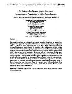
ACCEPTED MANUSCRIPT 153.8 from the Random

algorithm. The best code coverage is provided by ϵ-MOEA algorithm with 92.61%. In the second dataset, we notice the better solution of code coverage from the first dataset that's because of the second dataset despite having the less number of test case but with less than runtime cost and redundancy between the test cases.

162.5 176.2 140.7 171.4 194.5 166.9 149.8 135.4 191.1 118.8 167.4 163.6 118.7 131.0 172.3 157.4 168.7 161.1 161.6

RI PT

Sol #110 Sol #111 Sol #112 Sol #113 Sol #114 Sol #115 Sol #116 Sol #117 Sol #118 Sol #119 Sol #120 Sol #121 Sol #122 Sol #123 Sol #124 Sol #125 Sol #126 Sol #127 Sol #128 Sol #129

SC

In Fig 17 and Fig 18 the Scatter Charts shows relation between the Code Coverage and Redundancy and Cost for solutions that generated from the Random algorithm.

Fig 19. Code Coverage of All Algorithms for Dataset #2

TE D

M AN U

VII. CONCLUSION An efficient approach is proposed and applied to different four algorithms from MOEA Frame from the separate library with three fitness functions for Coverage, Cost, and Redundancy. Our Solution provides an efficient selection of test case for automated test cases generation tools that are suffering from low code coverage and the massive cost of the runtime of test cases cost. The experimental results demonstrate the accurate and efficient selection of test suits provided in each dataset with high code coverage percentage of 92.61%. We apply two different datasets of a different number of test cases to prove our concept of efficient selection of test cases considering the three objectives of maximizing Code Coverage and reducing the Cost and Redundancy.

AC C

EP

Fig 17. Random Coverage and Redundancy Rel. for Dataset #2

REFERENCES [1]

[2]

[3]

[4]

Fig 18. Random Coverage and Cost Rel. for Dataset #2 [5]

Finally, in Fig 19. The comparison code coverage chart between the four algorithms for dataset #2. Also, here we notice that small differences between the first three algorithms ϵ-MOEA, NSGAII, and SMSEMOA and the worst coverage

R. H. C. A. Gómez, C. A. C. Coello, and E. Alba, “A Parallel Version of SMS-EMOA for Many-Objective Optimization Problems,” Parallel Problem Solving from Nature – PPSN XIV Lecture Notes in Computer Science, pp. 568–577, 2016. “Basic Concepts,” Genetic and Evolutionary Computation Series Evolutionary Algorithms for Solving Multi-Objective Problems, pp. 1– 60. C. A. Coello Coello. Theoretical and Numerical Constraint-Handling Techniques used with Evolutionary Algorithms: A Survey of the State of the Art. Computer Methods in Applied Mechanics and Engineering, 191(11–12):1245–1287, January 2002. L. S. D. Souza, P. B. C. D. Miranda, R. B. C. Prudencio, and F. D. A. Barros, “A Multi-objective Particle Swarm Optimization for Test Case Selection Based on Functional Requirements Coverage and Execution Effort,” 2011 IEEE 23rd International Conference on Tools with Artificial Intelligence, 2011. Luciano S. de Souza, Ricardo B. C. Prudˆencio,and Flavia de A. Barros, “Multi-Objective Test Case Selection: A study of the influence of the Catfish effect on PSO based strategies”, Anais do XV Workshop de Testes e Tolerância a Falhas - WTF 2014.

SC

RI PT

Naujoks, and M. Emmerich, “SMS-EMOA: Multiobjective selection based on dominated hypervolume,” European Journal of Operational Research, vol. 181, no. 3, pp. 1653–1669, 2007. [10] K., H. Washizaki, et al. (2010). “Open Code Coverage Framework: A Consistent and Flexible Framework for Measuring Test Coverage Supporting Multiple Programming Languages”, In the 10thInternational Conference on Quality Software, QSIC, 2010, pp. 262-269.

M AN U TE D

[8]

EP

[7]

ACCEPTED MANUSCRIPT [9] N. Beume, B.

Chandraprakash Patidar, “Test Case Generation Using Discrete Particle Swarm Optimization Algorithm” International Journal of Scientific Research in Computer Science and Engineering, Jan- Feb-2013. Li, H. and Zhang, Q. \Multiobjective Optimization problems with Complicated Pareto Sets, MOEA/D and NSGA-II." IEEE Transactions on Evolutionary Computation, 13(2):284-302, 2009. S. Obayashi, Evolutionary multi-criterion optimization: 4th international conference: proceedings. Berlin: Springer, 2007.

AC C

[6]