1
An optimized variable-grid finite-difference method for seismic forward modeling Chunling Wu and Jerry M. Harris Department of Geophysics, Stanford University, Stanford, CA 94305, USA Abstract. An optimized fourth-order staggered-grid finitedifference (FD) operator is derived on a mesh with variable grid spacing and implemented to solve 2-D velocity-stress elastic wave equations. The idea in optimized schemes is to minimize the difference between the effective wave number and the actual wave number. As expected, this optimized variable-grid FD scheme has less dispersion errors than the variable-grid FD scheme based on Taylor series expansion with the same stencil. The accuracy of the proposed technique has been tested through the comparison with the analytical solutions and the regular-grid FD method based on Taylor series expansion. The effectiveness of the method is verified by its application for a thin-layer model. Key Words: optimized, variable-grid, finite-difference, seismic modeling 1. Introduction
2 FD
methods
have
historically
dominated
elastic
wavefield modeling in geophysics because of their flexibility in representing complex models and their computational efficiency. Recently, variable-grid FD techniques have been developed to avoid spatial oversampling when applied to multi-scale structures (Falk et al., 1996) or large-scale structures with high velocity contrasts (Pitarka, 1999). However, variable-grid FD methods developed based on the Taylor series approximation may suffer unacceptable dispersion. In this paper, we derive an optimized fourth-order staggered-grid FD operator on a mesh with variable grid spacing based on the idea of the DRP (dispersion-relation-preserving) scheme proposed by Tam and Webb (1993). The philosophy of the DRP method is to optimize the FD scheme coefficients by matching the effective wave number and the actual wave number over a particular wave number range. Comparison of the spectral properties between the optimized and the Taylor variable-grid FD schemes illustrates that the optimized scheme has less dispersion errors than the Taylor scheme (Pitarka, 1999) with the same stencil. We apply the proposed technique for a solution of 2-D velocity-stress elastic wave equations and demonstrate the method's accuracy and efficacy on some numerical examples. 2. Optimized variable-grid FD operator
3 The optimized variable-grid FD operator derived here is based on the idea of the DRP scheme proposed by Tam and Webb (1993). To illustrate the problem, the 1-D velocitypressure wave equations are considered (because spatial derivatives with respect to x, y and z are decoupled, the 1-D wave equation illustration will not lose generality):
∂v ∂p = ∂t ∂x ∂v ∂p , =K ∂x ∂t
ρ
(1)
where p and v are pressure and particle velocity, respectively; ρ is density and K is bulk modulus. Discretizing these equations by a staggered-grid FD mesh with variable grid spacing yields the scheme shown in Fig. 1. Suppose that the field variable g represents particle velocity v or pressure p. The approximation of the first-order spatial derivative ∂g/∂x by a fourth-order FD operator on a non-uniform grid of spacing dx is given by ∂g ( x ) = c1 g ( x + ∆1 ) + c2 g ( x − ∆2 ) + c3 g (x + ∆3 ) + c4 g ( x − ∆4 ) , ∂x
(2)
4 where ci are four coefficients to be determined. Spatial increments ∆i can be expressed in terms of the variable grid spacing dx (Fig. 2). After Fourier transform of equation (2), the effective numerical wave number of the FD scheme can be calculated by
k e = − i (c 1 e ik ∆ + c 2 e − ik∆ + c 3 e ik ∆ + c 4 e − ik ∆ 1
3
2
4
)
(3)
For the optimized FD scheme, the coefficients ci in equation (3) are chosen so that the effective wave number ke is close to the actual wave number k for a wide range of wave numbers. The coefficients ci are determined by imposing the condition that equation (2) is accurate to the third-order of ∆i through Taylor series expansion:
c1 + c2 + c3 + c 4 = 0 c1 ∆1 − c2 ∆ 2 + c3 ∆ 3 − c4 ∆ 4 = 1 (4)
c1 ∆21 + c2 ∆22 + c3 ∆23 + c 4 ∆24 = 0
This leaves one of the coefficients, e.g., c1, as a free parameter. This parameter is then chosen to minimize the integrated error E, defined as
E=λ
η
η
(k − Re(k e )) dk + (1 − λ ) (Im (k e ))2 dk , 2
0
0
(5)
5 where η is a predetermined number that gives the optimized range of wave numbers. The weighting coefficient λ, is used to balance the L2 norm of the truncation errors of the approximation of the real and imaginary parts of the effective numerical wave number to the actual wave number. The necessary condition used to minimize E is
∂E =0 ∂c1
(6)
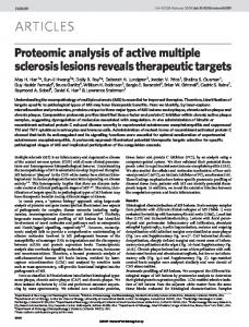
From equation (6), we can get c1 analytically. Then c2, c3, and c4 can be obtained from equation (4). We compare the spectral properties of this optimized variablegrid FD operator and the same order Taylor variable-grid FD operator (Pitarka, 1999) for different variable-grid meshes. Fig. 3 shows the relation between Re(ke)dxmin and kdxmin of both schemes for the stencil in Fig. 2(a) with the spacing ratio(r) between the coarse grid and the fine grid of 1, 3 and 6. The closer the curves are to the exact relation Re(ke)dxmin=kdxmin, the smaller the dispersion. Fig. 3 demonstrates that the optimized FD scheme has less dispersion errors than the FD scheme based on Taylor series expansion with the same mesh. In fact, the spectral resolution properties of the optimized FD scheme with the grid spacing ratio of 6 is much better than that of the Taylor variable-
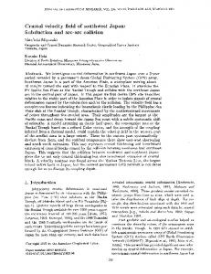
6 grid FD scheme with the same stencil and is even close to that of the Taylor regular grid FD scheme (spacing ratio of 1). This means that the optimized variable-grid FD scheme with large spacing ratios between two grid domains can give the same accurate results as the Taylor variable-grid FD scheme with small spacing ratios. Therefore, the optimized variable-grid FD technique can lead to either more accurate results with the same number of grid cells or more efficient calculations with fewer cells compared to the Taylor variable-grid FD method. 3. Applications of the optimized variable-grid FD operator To test the accuracy and the efficiency of the proposed optimized variable-grid FD scheme, we implement it for a solution of 2-D velocity-stress elastic wave equations. The following are two numerical examples. 3.1. Homogeneous model The homogeneous model with physical properties: Vp=2300 m/s, Vs=1100 m/s and ρ=2100 kg/m3, is shown in Fig. 4. We use this model to test the accuracy of the optimized variable-grid FD scheme when the grid spacing increases abruptly from 2 m to 6 m with a ratio of 3 in both x and z directions. The dashed line in Fig. 4 represents the boundary between the small grid spacing domain and the large grid spacing
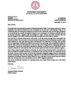
7 domain. A vertical dipole source (S), located at (450 m, 450 m), has a Ricker pulse with central frequency of 20 Hz. Receivers R1 and R2 are placed on the left- and the right-hand sides of the domain boundary, respectively. Figs. 5 and 6 present the comparison of the horizontal and vertical displacements calculated by the optimized variable-grid FD scheme with those obtained from the analytical solutions (Min et al., 2000) and the Taylor regular-grid FD scheme with a constant grid spacing of 2 m at receiver R1 and R2, respectively. The agreement among the three solutions is very good. Note that the FD schemes with variable- and regular-grid spacing give essentially identical results indicating both the reflection and the transmission artifacts from the domain boundary of the variablegrid FD scheme are negligible. 3.2. Thin-layer model The accuracy of the optimized variable-grid FD technique has been verified for a homogeneous region. Now we apply it for efficiently modeling wave propagation in a thin-layer model (Fig. 7). The size of the model is 6000 m × 2000 m. A waterfilled thin layer with 1 m thickness is imbedded in the model. The purpose of the modeling is to see if the effects of the thin fluid-filled layer can be observed in the seismograms. Table 1
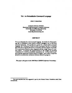
8 provides the physical properties of the model layers. The source, centered in y direction and located 600 m below the top, is a 20 Hz Ricker wavelet in pressure. Receivers are on both sides of and on the same level as the source. To resolve the thin layer with 1 m thickness, a very fine mesh (at least 0.2 m) is required. An equi-spaced mesh with sufficient resolution to describe the thin layer in this large-size model requires too much memory for most computers. For the optimized variable-grid FD method, the vertical grid spacing smoothly increases from 0.2 m to 5.4 m with a 7.2 m wide transition region. The horizontal grid spacing is 5.4 m throughout the grid. The total grid size for this variablegrid mesh is NX × NZ = 1225 × 517 which is only 4.08 percent of the total grid size for the regular-grid mesh with constant dx = 0.2 m in the entire model (NX × NZ = 30000 × 517); therefore, the variable-grid FD scheme saves over 95 percent computer memory for this model compared to the regular-grid FD scheme. Consequently, the computation time is reduced by more than 24 times. Fig. 8 shows the wavefield snapshots of horizontal and vertical particle velocities. Reflections and transmissions from the thin water-filled layer can be seen. No artifact is generated by smoothly varying spacing in the vicinity of the thin layer.
9 Seismograms of the horizontal and vertical particle velocity components are shown in Fig. 9. We can clearly see the reflected P- and S-waves from the thin layer in addition to the direct P-wave. This modeling study demonstrates that we need to include the effects of thin fluid-filled layers into the field data analysis. 4. Conclusions In this paper, an optimized fourth-order variable-grid FD operator has been derived and implemented for a solution of 2-D velocity-stress elastic wave equations. This optimized variablegrid FD scheme has less dispersion errors than the Taylor variable-grid FD scheme with the same stencil. Numerical examples demonstrate that the proposed technique can efficiently and accurately simulate wave propagation in large models with physically small features. Acknowledgments Financial support for this work was provided by the DOE through Lawrence Berkeley National Laboratory. References
10 Falk, J., Tessmer, E., and Gajewski, D. G., 1996. Tube wave modeling by the finite-difference method with varying grid spacing. PAGEOPH, 148: 77–92. Min, D.J., Shin, C., Kwon, B.D., and Chung, S., 2000. Improved frequency-domain elastic wave modeling using weightedaveraging difference operators. Geophysics, 65: 884–895. Pitarka, A., 1999. 3D finite-difference modeling of seismic motion using staggered grids with nonuniform spacing, Bull. Seismol. Soc. Am., 89: 54–68. Rector, J.W., Zhang, L., and Hoversten, M.G., 2002. Optimized coefficient finite difference scheme for wave equation, paper presented at SEG Post-Convention Workshop--Advances and limitations in numerical modeling of wave propagation in challenging structures, 72nd Ann. Internat. Mtg., Soc. Expl. Geophys., Salt Lake City, USA. Tam, C.K.W., and Webb, J.C., 1993. Dispersion-relationpreserving difference schemes for computational acoustics, Journal of Computational Physics, 107: 262–281. ______
11 Chunling Wu and Jerry M. Harris, Department of Geophysics, Stanford
University,
Stanford,
CA
94305,
USA.
(
[email protected])
Figures Fig. 1. (a) Schematic representation of unit cells and (b) the variable grid spacing. Fig. 2. Grid nodes with variable spacing. ∆i (i = 1, 4) are used to calculate the FD operator centered between (a) the nodes i and i+1 and (b) that centered at the node i. Fig. 3. Re(ke)dxmin versus kdxmin of the optimized and Taylor variable-grid FD schemes for the stencil in Figure 2(a). r represents the spacing ratio of the coarse grid to the fine grid. The exact relation is Re(ke)dxmin=kdxmin. Fig. 4. Homogeneous model. Fig. 5. Comparison of optimized variable-grid FD method (OVGFD) with the analytic solutions and the Taylor regular-grid FD scheme (TRGFD) at receiver R1: (a) horizontal displacement; (b) vertical displacement.
12 Fig. 6. Comparison of optimized variable-grid FD method (OVGFD) with the analytic solutions and the Taylor regular-grid FD scheme (TRGFD) at receiver R2: (a) horizontal displacement; (b) vertical displacement. Fig. 7. Thin-layer model. Fig. 8. Snapshots of horizontal particle velocity (Vx) and vertical particle velocity (Vz) components of the thin-layer model. Reflections and transmissions from the thin layer can be seen. Fig. 9. Seismograms of horizontal particle velocity (Vx) and vertical particle velocity (Vz) components of the thin-layer model. Reflected P- and S-waves from the thin water-filled layer are observed in addition to the direct P-wave.
Table 1. Material properties of the thin-layer model
No.
Vp(m/s)
Vs(m/s)
ρ(kg/m3)
1
3000
1700
2300
2
1500
0
1000
13
Fig. 1. (a) Schematic representation of unit cells and (b) the variable grid spacing.
Fig. 2. Grid nodes with variable spacing. ∆i (i = 1, 4) are used to calculate the FD operator centered between (a) the nodes i and i+1 and (b) that centered at the node i.
14
Fig. 3. Re(ke)dxmin versus kdxmin of the optimized and Taylor variable-grid FD schemes for the stencil in Figure 2(a). r represents the spacing ratio of the coarse grid to the fine grid. The exact relation is Re(ke)dxmin=kdxmin.
Fig. 4. Homogeneous model.
15
Fig. 5. Comparison of optimized variable-grid FD method (OVGFD) with the analytic solutions and the Taylor regular-grid FD scheme (TRGFD) at receiver R1: (a) horizontal displacement; (b) vertical displacement.
16
Fig. 6. Comparison of optimized variable-grid FD method (OVGFD) with the analytic solutions and the Taylor regular-grid FD scheme (TRGFD) at receiver R2: (a) horizontal displacement; (b) vertical displacement.
Fig. 7. Thin-layer model.
17
Fig. 8. Snapshots of horizontal particle velocity (Vx) and vertical particle velocity (Vz) components of the thin-layer model. Reflections and transmissions from the thin layer can be seen.
18 Fig. 9. Seismograms of horizontal particle velocity (Vx) and vertical particle velocity (Vz) components of the thin-layer model. Reflected P- and S-waves from the thin water-filled layer are observed in addition to the direct P-wave.