An ordered examination of influence diagrams - Semantic Scholar

An Ordered Examination of Influence Diagrams Ross D. Shachter Department of Engineering-Economic Systems, Stanford University, Stanford, Calif0rn ia 94305-4025

Influence diagrams are a directed network representation for decision making under uncertainty. The nodes in the diagram represent uncertain and decision variables, and the arcs indicate probabilistic dependence and observability. This paper examines the graphical orderings underlying the influence diagram and the primitive interchange operations that can reorder the network. These operations are sufficient to determine the maximal independent set and minimal relevant sets for any given inference problem, and a linear time algorithm is developed to obtain those sets. This framework is also used to examine and explain properties of the time structure of general influence diagrams with decisions. 1. INTRODUCTION

The influence diagram is a general, abstract, intuitive modeling tool that is nonetheless mathematically precise. Influence diagrams are directed graph networks, with different types of nodes representing uncertain quantities, decision variables, deterministic functions, and value models. The arcs have different meanings, depending on the type of node they go into: “Conditional” arcs into random nodes show conditional dependence, whereas “informational” arcs into decision nodes indicate which variables will be observed before an alternative must be chosen. The conditional arcs in the influence diagram reveal both obvious and subtle forms of conditional independence. The principle of d-separation [3,10,14,19] extends the intuitive notion of separation in the undirected graph to its less obvious form in the directed graph representation. This can be further specialized to the directed graph by introducing deterministic functions, which cannot be represented at all in the undirected graph [3,5,16]. Another important property is the set of relevant nodes, those nodes for which information must be provided in order to compute probabilistic inference [5,16]. Although relevance is closely related to independence and can be detected in similar topological analysis, it is quite different. Both conditional independence and relevance can be detected using simple, efficient procedures 141. NETWORKS, Vol. 20 (1990)535563

01990 John Wiley & Sons, Inc.

CCC 0028-3045/90/050535-029$04.00

536

SHACHTER

In this paper, the analysis of influence diagram structure is performed in its underlying partial orderings: the chance ordering of the conditional arcs and the decision ordering of the informational arcs. Three primitive interchange operations for reordering the influence diagram graph allow us to transform the given influence diagram into one with a different chance ordering. This allows us to explore both the conditional independence and relevance implicit in the probabilistic ordering and the time structure captured in the decision ordering. It also demonstrates the fundamental nature of the main interchange operation, arc reversal, which is the influence diagram representation for Bayes’ theorem [8,13,16]. Section 2 explains the basic properties of partial orderings, whereas Section 3 defines conditional independence on the undirected graph. The probabilistic influence diagram is introduced in Section 4, and its interchange operations are derived in Section 5. These results are then applied in Section 6 to recognize the independence and relevance in inference problems, and in Section 7, to analyze the time structure in influence diagrams with decisions. Finally, Section 8 presents a summary and conclusions. 2. PARTIAL ORDERINGS

Some basic properties of partial orderings are represented in this section. This provides a unifying framework for the analysis of the influence diagram structure. A key result is the “Interchange Algorithm,” which transforms an arbitrary listing of the elements of a set into a list that satisfies a given partial ordering , with a minimal amount of rearrangement. The simple abstraction of the partial ordering captures our desired manipulation to the influence diagram. The relation ‘‘5’’is called a binary relation on a finite set of elements N if it compares pairs of elements from N . The following properties are commonly defined for binary relations [2]: reflexive: x 5 x for all x E N ; transitive: if x Iy and y 5 z , then x 5 z for all x, y , and z E N ; antisymmetric: if x 5 y and y 5 x, then x is y for all x and y E N ; and complete: x 5 y and/or y 5 x for all x and y E N . The relation 5 is a partial ordering if it is reflexive, transitive, and antisymmetric. A partial ordering is a total ordering if it is also complete. For convenience, several corresponding relations are defined for elements x and y € N :

x < y if x S y and x is not y ; x 2 y if y ~ x and ; x > y if y 5 x and x is not y . If

5

is a partial ordering, then the relation

2

is a partial ordering, but both

< and > are not partial orderings because they are not reflexive. The definitions of these binary relations can be extended to compare and

AN ORDERED EXAMINATION OF INFLUENCE DIAGRAMS

537

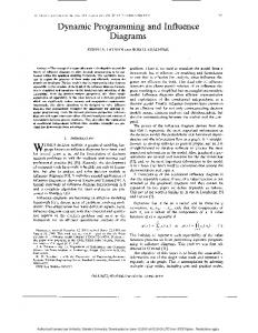
define sets. Let Y and Z be subsets of N . For the reflexive relations, 5 and 2, Y 5 2 means that for every y E Y there is some z E 2 such that y 5 z ; for the nonreflexive operators, < and >, Y < Z means that y < z for every y E Y and z E Z . Now define set-valued functions 5 b}= {x E N : x Iy } and similar functions for 2 z for some z > s x but there is no z > s y for which y > 2 z , perform an interchange operation on (x,y) in s. The comparison in the Interchange Algorithm is more complicated than would be necessary if 5 , were a total ordering. In that case, an interchange operation should be performed on (x,y) if and only if x >2y, and the ordering s2 is determined regardless of sl. Consider, however, the case of three elements x, y, and z , with s1 = (xy z ) and z c2x.The sequence s1 is shown in Figure l(a) and the ordering s2is shown in Figure l(b). There are two adjacent pairs in the sequence sl, (x,y) and ( y , z ) , and although neither one satisfies x >2y nor y >2 z , clearly x and z are in the wrong order. The comparison in the algorithm, however, recognizes that there should be interchanges, first with (x,y), and then with ( x , z ) , resulting in the final sequence s2 = (y z x), shown in Figure l(c). Let s2 be the final sequence s in the algorithm, s2 = s2U (sl\>2), so s2 is consistent with s2.Since the same two nodes will only participate once in an interchange, in the worst case there would be IN1 (IN1 - 1) interchange operations. Because the interchange operation is only performed on (x,y) if neither x s2y nor x y, every intermediate sequence s will be consistent with fl s2

FIG. 1. The interchange algorithm.


539

and s1 r l s,. (This property of the interchange algorithm is called stability.) In the example drawn in Figure 1, y < L in the final sequence, since that ordering from the original sequence can be maintained without violating the target ordering. These results are summarized in the following proposition. Proposition 1. Interchange Algorithm Given any initial partial ordering s1and target partial ordering s2,a sequence consistent with s1can be reordered into a sequence consistent with s2 through a finite number of interchange operations. Furthermore, using the Interchange Algorithm, every intermediate sequence will be consistent with

s1n I,. 3. GENERAL CONDITIONAL INDEPENDENCE

Conditional independence is defined in this section in terms of a “separation property” in a undirected graph. From this definition, we can derive the interchange operations on the influence diagram. These operations would apply to any independence relation that satisfied undirected graph separation, although, clearly, probability is our main concern. Suppose that X , Y , and Z are there disjoint sets of nodes in an undirected graph. Sets X,Y,and Z are said to satisfy the (undirected) separation property if every path between X and Y contains a node from 2. The abstract property of conditional independence can be represented through this separation: An undirected graph is valid if X is conditionally independent given 2, written X lL YI 2, whenever X , Y , and 2 satisfy the separation property in the graph. Conversely, if X IL YI Z , then there is some graph in which X,Y,and Z satisfy the separation property. For example, if the undirected graph in Figure 2 is I (XU Y), and (W U X) lL 21Y , but not (necessarily) W lL Z/X. valid, W lL Z Two useful properties that follow immediately from the separation property are

I Z;and Symmetry: X lL YI Z if and only if Y lL X Overlap: X lL Y 1 Z if and only if X V (YU 2)12. These will be used extensively throughout this paper. Only one other property, the (undirected) combination property is needed to extend this definition of conditional independence, by inferring a new graph from two other graphs. Although many other useful properties follow [1,10], the proofs in this paper will be based directly on the separation and combination properties.

@:g@

FIG. 2. Conditional independence in an undirected graph.

540

SHACHTER

Axiom 1. Undirected Combination Property Given two valid undirected graphs, with node sets U and V , respectively, where U C V , let X = V\ U and let Y be those nodes in U that are adjacent to X in the second graph. A new graph, logically implied by the other two, can be formed from the first graph by adding nodes X and arcs between all nodes in X U Y .

In the most important case of independence, probabilistic independence, X lL Y 12 if and only if P{XI Y,Z} = P{XI Z} for any 2 such that P{Z}> 0. A degenerate case of that, “functional” independence, will be described in the next section. It arises when X IL Nl 2,that is, X is even independent of itself, conditional on 2.Unfortunately, although the separation property can be used to analyze functional independence, such independence cannot be represented in the undirected graph. 4. PROBABILISTIC INFLUENCE DIAGRAM

The probabilistic influence diagram, which only models random variables, is introduced in this section. The separation property of conditional independence from the previous section is now applied to a directed graph specification of a model. In this framework, we can represent deterministic functions and recognize some of the simple independencies that arise when some of the variables are observed. The full influence diagram, with decision nodes and a value node, is presented in Section 7. An influence diagram is a network on a directed acyclic graph. Each node in the graph represents a variable in the model. This variable can be an uncertain quantity, a decision to be made, or a criterion for choosing decisions. When a diagram consists of only uncertain quantities, it is called a probabilistic influence diagram. Assign indices to the nodes and variables in the influence diagram, so that the nodes are given by N = (1, . . . ,n} and they correspond to variables XI, . . . ,Xn.Each variable X, has a set of possible outcomes 0, and a conditional probability distribution T,over those outcomes. The conditioning variables for that distribution have indices in the set of conditional predecessors, C ( j ) C N , the parents of node j in the graph. If the distribution is unconditional, then C ( j ) is the empty set, 0,and j is a source node. As a convention, a lower case letter represents one node in the graph and an upper case letter represents a set of nodes. If J C N is a set of nodes, then X , denotes the vector of variables indexed by J and lRJ denotes the cross product of their outcomes XlEJCl1. For example, the conditioning variables for X, are Xco, and they have outcomes RcO), so that

The conditional predecessors for a set of nodes J , C ( J ) , is the union of their parents,


541

C ( J ) := UjEJ C ( j ) . Likewise, let S(J) be the set of children or (direct) successors to the nodes J ,

S(J) := { j E N : J n c(j)#

0).

There are two types of variables in a probabilistic influence diagram. The value of a deterministic variable is known with certainty once the values of its conditioning variables have been observed, although there might be uncertainty about its value otherwise. On the other hand, a probabilistic variable’s value might be uncertain, even when the values of its conditioning variables have been observed. Probabilistic nodes are drawn in the diagram as ovals, whereas deterministic nodes are drawn as double ovals. Let F be the set of deterministic (functional) nodes and C be all of the (chance) nodes in the probabilistic influence diagrams, both probabilistic and deterministic. When the influence diagram graph is completely drawn, including the identification of deterministic nodes F , then the diagram is said to be partially speciJied. If it also has outcomes and conditional probability distributions assigned for all of its variables, then it is fully spec@ed. A partially specified the chance ordering, on the influence diagram induces a partial ordering sC, set of nodes N . Define i scj if and only if there is a (possibly empty) directed path from i to j for all i and j E N in a probabilistic influence diagram. We assume that there are no directed cycles, so the chance ordering sCis a partial ordering. Given a sequence s on the nodes N , a partially specified influence diagram is a list of conditional predecessor sets and deterministic flags corresponding to s. In order for s to be consistent with sC, directed cycles are not permitted, and thus C ( j ) C < J j ) for all nodes j . The conditional predecessor sets state strictly ordered independence with respect to s, that is,

If Xiis deterministic, then it is conditionally independent of all of the variables X , given its conditioning variables Xco.),

As a result, it can be represented as a function of the values of its conditioning variables, fi: SZ,), --., SZj, and corresponds to a degenerate conditional probability distribution. It would be much more convenient if the independence in the graph did not depend on the exact sequence in which the nodes were ordered, but only on their partial order. As will be shown in the next section, partially ordered independence implies that

for any sequence s consistent with sC.

542

SHACHTER

Whenever some of the variables in the diagram are observed, there might be new conditional independencies. Since all of the variables in the network are conditioned on the observed values, there is not need to include them in the sets of conditioning variables. This is summarized in the following proposition ~71. Proposition 2. Evidence Absorption If the variables X K have been observed in a probabilistic influence diagram, then all of the outgoing arcs from their associated nodes can be deleted without changing any of the assumptions of conditional independence.

Operationally, the observed variables no longer condition their children once their observations have been instantiated into their children’s conditional distributions. Since their values are known, they are now independent of all of the other variables in the model. Another case in which a variable’s value is known is when it corresponds to a deterministic source node. If deterministic node j has no parents, C ( j ) = 0, then, by definition,

x,fi XN, and Xiis independent of all the variables, including itself. In this case, it can be treated just like an observed variable, instantiated into its children’s distributions, and then removed from their conditioning sets. Proposition 3. Deterministic Absorption If a deterministic variable Xihas no conditioning variables, then the outgoing arcs from its associated node can be deleted without changing any of the assumptions of conditional independence.

Although the starting diagram could contain deterministic source nodes, previous applications of evidence and deterministic absorption might have eliminated the arcs into a deterministic node. It is useful to define the functional successors, FL, of the nodes K to correspond to those variables that become conditionally independent of all other variables given X K [3]:

Fk

= {i E N

Xili XNIXK}.

Note how strong this definition is, since these variables must even be independent of themselves given X K . Unfortunately, we are unable to detect all elements in F i by examining the graph, so let FK be the (graphically detectable) functional successors of K , those elements of FL that can be logically determined from the influence diagram graph. Clearly, FK includes the nodes in K and any deterministic nodes whose parents are all in FK. By repeated application of evidence and deterministic absorption, we obtain the recursive formula [5]

The set FK can be obtained efficiently by making a single pass through the


543

influence diagram in graph order, performing evidence and deterministic absorption. 5. INTERCHANGE OPERATIONS FOR THE PROBABILISTIC INFLUENCE DIAGRAM

The arcs in a probabilistic influence diagram induce a partial ordering, the They also explicitly represent some of the conditional chance ordering I,. independence in the model in the form of strictly ordered independence. In order to recognize additional independence, such as partially ordered independence, we need to develop interchange operations so that we can employ the Interchange Algorithm to reorder the diagram. There are three interchange operations, “Null Reversal,” “Arc Reversal,” and “Deterministic Propagation.” Since these operations will allow us to detect all of the independence in the network, they are as fundamental as the undirected graph separation property. Before proving partially ordered independence, we must first derive some results about noncomparable nodes. Consider the influence diagram drawn in , Figure 3(a). It shows two nodes i and j that are noncomparable under I,that is, there is no directed path between i and j in either direction. There is at least one sequence consistent with sCin which (iJ) are adjacent and at least one in which (jj)are adjacent. Switching from one of these orderings to the other will be called “Null Reversal.”

FIG. 3. Null Reversal.

544

SHACHTER

Theorem 1. Null Reversal If (i,j) are adjacent in a sequence s1on N and i 4 C ( j ) in an influence diagram with strictly ordered independence with respect to sl, then strictly ordered independence is satisfied with respect to the sequence s2, obtained by interchanging i and j in sl.

Proof. Because ( i J ) are adjacent in s1 and i SE C ( j ) it must follow that i and j are and both sequences s1 and s2 noncomparable with respect to the ordering sC, are consistent with sC. Letting K = C(i) r l CG), J = C(i)\K, L = C(j)\K, and M =