This paper presents and proposes an optimization model for railway power ... The program is implemented in GAMS (General Algebraic Modeling. System).
An SOS2-based moving trains, fixed nodes, railway power system simulator L. Abrahamsson and L. S¨oder KTH Royal Institute of Technology, Sweden
Abstract This paper presents and proposes an optimization model for railway power supply system simulations. It includes detailed power systems modeling, train movements in discretized time considering running resistance and other mechanical constraints, and the voltage-drop-induced reduction of possible train tractive forces. The model has a fixed number of stationary power system nodes. The proposed model uses SOS2 (special ordered sets of type 2) variables to distribute the train loads to the two most adjacent power system nodes available. The impact of the number of power system nodes along the contact line and the discretized time step length impacts on model accuracy and computation times are investigated. The program is implemented in GAMS (General Algebraic Modeling System). Experiences from various solver choices are also presented. The train traveling times are minimized in the example. Other studies could, e.g. consider energy consumption minimization. The numerical example is representative for a Swedish non-centralized, rotary-converter fed railway power supply system. The proposed concept is however generalizable and could be applied for all kinds of moving load power system studies. Keywords: optimization, railway, power systems, load flow, special ordered sets of type 2, MINLP, moving loads, simulation, driving strategies
1 Introduction 1.1 Background and Motivation In [1] the main differences between public power systems and railway power supply systems are extensively discussed and explained. Typically, the loads are neither fixed power or fixed current, they vary heavily. It is also one of the earliest publications where the problem with moving nodes connected to the moving loads are ventilated. It was proposed to replace loads along a catenary section with loads at the substation(s) feeding the section. The number of nodes in [1] was successively increased, but kept fixed to the number and their locations in each study, like in this paper. The main differences between this paper and [1] is the use of SOS2 (Special Ordered Sets of type 2) variables for alleviating the use of the idea presented in [1], and to introduce optimization into the model. SOS2 variables are, in vector form, nonzero for at most two adjacent elements in the vector. SOS2 is typically used for sampling nonlinear functions into piecewise linear ones. The proposed model uses SOS2 variables to distribute the train loads to the two most adjacent power system nodes available. The application of SOS2 presented in this paper is as far as the authors know completely new and previously unpublished. Besides that keeping the number and the location of the nodes fixed simplifies the systematic bookkeeping of simulation results [1, 2], also the admittances of the system become more of the same orders of magnitude not hazarding admittances close to zero or infinity, which the modeling solution in [2] rather amplifies than alleviates. In [1] various algorithmic methods are discussed, whereas in this paper standard commercial off-the-shelf solver software are used. Also the challenge of finding the ultimate starting iteration points is discussed in [1]. Typically, when simulating railway power supply systems with moving loads, the power system has to change in topology for each time step [2–4] introducing a complicated bookkeeping of train numbers, train locations, node numbers, which trains are in traffic or not, which nodes coincide and should be merged or not, etc. There are ways of getting rid of this problem. One is presented in [2], where the bookkeeping is given a clearer structure by graph-representation. However, in [2], all trains are present in the power system all the time which would tend to increase the system size. Moreover, [2] is designed to access train power consumption from an external program, and as in [3, 4] each time step is made a separate simulation.
1.2 Contribution The main contributions of this paper are that the model: • ... has a fixed number of stationary power system nodes, • ... is formulated as one single optimization problem, which – ... allows combined studies of optimal driving strategies and power system operation, – ... offers a surveyable modeling framework contained in one objective and a set of constraints – ... allows more detailed and realistic studies – ... makes it possible solving the problem in different hardware and software environments, like e.g. in supercomputers, without considering communication between different parts of the model Such parts would be power flow computations, braking strategies computations, power system topology and train speed and location updates, and possibly next time steps train power consumption levels. In contrast to railway power supply system (RPSS) simulator models where the power system operation of each snapshot in time acts as there where no future and no past, the model in this paper optimizes electrically and mechanically also in the temporal dimension. This is typically useful for studies of on-vehicle [5–7] and railside energy storage [5, 8,9]. When is it optimal to charge/discharge? Sometimes it might be wise to wait with the discharge until the really big load passes by, rather than using it on the first voltage dip spotted. 1.3 Paper Content This paper presents and proposes an optimization program model for railway power supply system simulations, including train movements in discretized time considering running resistance and other mechanical constraints, and the voltage-drop-induced reduction of possible train tractive forces. In the numerical example, the impact of the number of power system nodes along the contact line and the the discretized time step length impacts on model accuracy and computation times are investigated. The program is implemented in GAMS [10]. Experiences from various solver [11] choices are also presented. The train traveling times are minimized in the example. The numerical example is representative for a Swedish non-centralized, rotary-converter fed railway power supply system with BT-type contact lines. The proposed concept is however generalizable and could be applied
to all kinds of moving load power system studies.
2 The Model Given the catenary type, catenary lengths, system topography, the number and placement of desired electrical nodes sampling the catenary, the admittance matrix is created. It has been assumed that the trains consume no reactive power. Moreover, auxiliary power load and internal train losses are neglected. The model studied in the numerical example is constrained to one doublyfed catenary section. The concept is however generalizable. The maximal number of possible time-steps are calculated such that even severely delayed trains will make it to their destinations before time is up. The model is simplified such that the adhesive train mass is assumed to be the mass of the train for braking, coasting, and motoring. Therefore, also consideration of rotational inertia in the wheel sets and in the locomotive is unconsidered. Slippage is also unconsidered since the adhesive force between wheel and rail is assumed to always be large enough to use the entire motoring force as tractive force. The model is simplified in this way because the focus of this paper is to promote the idea of fixed-node models for moving load power systems – not to have exact mechanical models of the train-rail interaction. For proper models of train-rail interaction, c.f. [12] and for less simplified models including the power system, c.f. [3]. Moreover, train tractive resistance due to curves and grades of the track are not implemented in this model, the rail is assumed to be straight and flat. Due to limited space, the model is described in words only. Train acceleration depends on tractive force, resistive force, and braking force respectively. Velocity changes in time step δ + 1 are computed using the accelerations of time step δ, whereas position changes, besides accelerations of time step δ, also depend upon velocities in time δ. The train resistive force follows the classical second order polynomial [12] when the train is moving, and is set to zero otherwise. There are a number of constraints involving binary variables in order to determine when the train brakes, have braked, drives, and stands still – some of these states can be combined, others not. The binaries allows the braking force to be nonzero when braking, and conversely the tractive force to be nonzero when driving. The tractive force is bounded above by the train motors constant force curve, its constant power curve, and the constant power curve that is lowered for catenary voltages below nominal voltage (here, 15 kV). The brake-point-velocity between constant force
and constant power is 78 km/h for nominal and higher catenary voltages. The train positions are using the SOS2 variable projected proportionally to the two closest electrical nodes. The proportions are used to distribute the train loads to the power system, and to estimate the voltage levels at the pantograph. Train tractive power is calculated by the product of tractive force and train speed assuming lossless trains. The power flows are computed using classical AC load flow models, and the railway is fed two-side by Q48/Q49 [13] rotary converters, 6 in each station. The objective is to minimize the trains position deviations from the end station position, i.e. to make the train reach its final destination as fast as possible.
3 Numerical Examples and Results In all the studies made, the catenary nodes were located equidistantly. The model as such does however allow non-uniform spatial sampling of the catenary. 3.1 Generally
1
1
0.5
0.5
0
0 20 40 time (min)
60
0
50 100 position (km)
150
(a) Normalized curves plotted against (b) Normalized curves plotted against train time. position.
Figure 1: Electrical and mechanical properties of the train plotted against time and position respectively. The example is taken from a study with a 150 km BT catenary section, 1 train, 1 minute time step length, 31 catenary nodes. In Figure 1a the resulting curves of tractive force, pantograph voltage,
velocity, position, and power consumption as a function of time is displayed, whereas tractive force, pantograph voltage, velocity, and power consumption are presented as functions of train position in Figure 1b. In Figure 1, the tractive force is plotted as a solid black line, train voltage is plotted as a dotted black line, train velocity is plotted as a dash-dotted black line, train position is plotted as a solid dark grey line, and train active power consumption is plotted as a dashed black line. All the curves are normalized. The tractive force is scaled by 275 kN, the train voltage is expressed in p.u., the train velocity is scaled by 160 km/h, train position is scaled by 150 km, and train power consumption is scaled by 5.958 MW. The base voltage is 16.5 kV. Studying Figure 1, one can see that there are two flat levels of the tractive power curve, the higher one represents the maximal possible power consumption of the train which is 5.958 MW, computed by the upper limit of the constant power constraint 275 · 103 · 78 Fmax · 78 = = 5.598 MW, 3.6 3.6
(1)
whereas the lower one, at 5.555 MW originates from the running resistance at the speed limit � �v �2 � vmax vmax max 15400 + 279 + 49.2 = 3.6 3.6 3.6 (2) � �2 ! 160 160 160 15400 + 279 + 49.2 = 5.555 MW. 3.6 3.6 3.6 The lowest value of the tractive power, due to catenary voltage drops and reduced tractive performance, is 5.214 MW. In Figure 2, the catenary node voltages are illustrated over time in a gray scale matrix, where the white rectangles represents 1.000 p.u. and where the lowest value is 0.794 p.u. and is represented by black rectangles. The lowest voltage is registered when the train is in the middle of the catenary section. For each time step, the lowest voltage is registered where the train is located. 3.2 The impact of time step size variations Since the problem is extremely time consuming to solve on personal computers when using small time step sizes and catenaries longer than 100 km, a 50 km section is studied. The studied time step sizes are of 0.2, 0.5, 1, and
1 0.98 5 0.96 0.94
node number
10
0.92 15
0.9 0.88
20 0.86 0.84
25
0.82 30
0.8 10
20
30 40 time [min]
50
60
Figure 2: Voltages at the catenary nodes. All 31 nodes, over 65 minutes, 150 km catenary section. Voltage levels in p.u.
Table 1: The impact on computation times and results on discretization time step. Results from a 50 km section and one single train trafficking. Time Step (min)
Objective values
Computation times (s)
2
114.33
11.043
1
126.08
18.647
0.5
130.65
158.24
0.2
134.02
5713.1
2 minutes respectively and the catenary is represented by 10 equidistantly located nodes. The computational times and the objective values for the different step sizes are summarized in Table 1. Reduced time step sizes lead to increased train traveling times as well as computational times.
Computation Times (s)
Computational Times (s)
3.3 The impact of catenary node density
100
50
0
20 40 Catenary Nodes
104
103
102 10 20 30 Catenary Nodes
40
(a) Comparison of computation times for (b) Comparison of computation times for 50 km catenary, one train, and 3 to 53 150 km catenary, one train, 3 to 40 catenary catenary nodes. nodes.
Figure 3: Computational Times in s for various number of catenary nodes. For 1 minute time steps, 1 train, and 50 km catenary, the train traveling time results are exactly equal regardless of the number of catenary nodes. This is because there is no need for detailed power system models if the grid is strong in comparison to the load, and energy or power consumption is not studied. In Figure 3a, the number of catenary nodes is varied from 3 to 40 and there is a clear linear trend in the computation times for increased number of nodes. For the 1 minute time steps, one single train, and 150 km catenary case, the train traveling time results slowly converge to an objective slightly greater than 410 when the number of catenary nodes are 35 or more, c.f. Figure 4. The trend is that for increased number of nodes, the traveling times increase. The computational times increase dramatically and then settle around 105 seconds, illustrated in Figure 3b. 3.4 Solver choice impacts In most of the simulations, and all the here presented numerical results, the solver SBB [11] has been used. SBB seems to be the solver that works best with this kind of model. SBB seems on the other hand to very easily find local undesired optima, so lots of helping constraints was needed to be added.
415
410
Objective Value
405
400
395
390
385
5
10
15
20 25 Catenary Nodes
30
35
40
Figure 4: Convergence for the 150 km case study and increasing numbers of catenary nodes BONMIN [11] has also been tried out, resulting in the same solutions as SBB, but with significantly longer computation times, e.g. what took about 15 seconds in SBB took about 20 minutes in BONMIN. That test was made on a system with a 20 km catenary. 3.5 Alternative Objective Functions Some other objectives were tried out that logically also would aim at minimizing train traveling times. Experiments have been done minimizing negative velocities, the summed squares of the tractive and the braking forces, and the sum of the driving and braking binary indicator variables. These experiments resulted in faster computation times, and slightly longer train traveling times, but edgy tractive force curves indicating an unrealistic and undesired solution.
4 Conclusions A useful way of modeling a moving load RPSS as a fixed-node optimization problem has been presented and proven to produce exact and trustworthy results. Computational times increase significantly when voltage drops start to affect train traffic performance and when time step sizes drop. The model has uniform time steps, but is general in the catenary nodes discretization allowing nonuniform sampling. Electrical accuracy is increased by denser located catenary nodes, and mechanical accuracy by smaller time step sizes. Accuracy has a price – computer time.
5 Discussions and Future Work As long as the studies only focus on possible train tractive performances, there is no accuracy increase to have many electrical nodes along the catenary when the grid is comparatively strong in relation to the loads. When however studying weaker or heavier loaded grids node densities matter. 5.1 Future Studies A nonuniform spatial sampling, where e.g. sampling denser in the middle of the catenary section, where the voltage drops are more likely to be substantial, could be expected to create a good tradeoff between accuracy and computational times. In this paper, train traveling times have been minimized indirectly by maximizing the summed train positions. One can also, e.g. minimize energy consumption, and peak power consumption. Within the existing modeling framework, optimal operation control of converters could be added. These converters could be the ones feeding the railway from the public grid or a railway feeding transmission line [14], converters regulating charge/discharge of energy storage, or the on-train converters. 5.2 Solver Choice and Modeling It could be of interest rewriting the SOS2 variable formulation as an equivalent system of binary variables in order to see if the model can be solved well by other solvers not as adapted to the SOS2 variables as the SBB solver seems to be. It can be expected that solvers like BONMIN are more
accurate, but demands extensive computational resources. Integer variables potentially slow down optimization problems significantly, especially problems with nonlinear constraints. Binary variables in vector form that only change value once could be reformulated as SOS1 variables. SOS1 variables have been tried out during the model development process to model trains that have started to brake and trains that have finally stopped. The computational times were not significantly reduced then. The potential in using SOS1 variables instead of binaries could however still be further studied, also to indicate that a train has started from standstill position. Typically for this problem is that many different physical units are used, scaled and unscaled. Therefore, it is expected that the numerical performance would be improved by scaling [15, 16].
References [1] Talukdar, S.N. & Koo, R.L., The analysis of electrified ground transportation networks. IEEE Transactions on Power Apparatus and Systems, 96(1), pp. 240–247, 1977. [2] Arboleya, P., Diaz, G. & Coto, M., Unified ac/dc power flow for traction systems: A new concept. IEEE Journal of Vehicular Technology, 61(6), pp. 2421–2430, 2012. [3] Abrahamsson, L., Railway Power Supply Models and Methods for Long-term Investment Analysis. Technical report, Royal Institute of Technology (KTH), Stockholm, Sweden, 2008. Licentiate Thesis. [4] Boullanger, B., Modeling and simulation of future railways. Master’s thesis, Royal Institute of Technology (KTH), 2009. [5] Barrero, R., Tackoen, X. & Mierlo, J.V., Quasi-static simulation method for evaluation of energy consumption in hybrid light rail vehicles. Vehicle Power and Propulsion Conference, 2008. VPPC ’08. IEEE, pp. 1–7, 2008. [6] Ciccarelli, F., Iannuzzi, D. & Tricoli, P., Control of metro-trains equipped with onboard supercapacitors for energy saving and reduction of power peak demand. Transportation Research Part C: Emerging Technologies, 24, pp. 36–49, 2012. [7] Iannuzzi, D. & Tricoli, P., Speed-based state-of-charge tracking control for metro trains with onboard supercapacitors. Power Electronics, IEEE Transactions on, 27(4), pp. 2129–2140, 2012. [8] Iannuzzi, D., Lauria, D. & Tricoli, P., Optimal design of stationary
[9]
[10] [11] [12]
[13]
[14]
[15] [16]
supercapacitors storage devices for light electrical transportation systems. Optimization and Engineering, 2011. DOI: 10.1007/s11081-0119160-4. Iannuzzi, D., Ciccarelli, F. & Lauria, D., Stationary ultracapacitors storage device for improving energy saving and voltage profile of light transportation networks. Transportation Research Part C: Emerging Technologies, 21(1), pp. 321–337, 2012. GAMS, Welcome to the GAMS Home Page!, 2008. http://www.gams. com. GAMS, Solver descriptions, 2011. http://www.gams.com/solvers/ solvers.htm. Lukaszewicz, P., Energy Consumption and Running Time for Trains. Ph.D. thesis, Division of Railway Technology, KTH, Stockholm, Sweden, 2001. Kols, H., Frequency Converters for Railway Feeding (original title in Swedish). Technical Report BVH 543.17000, Swedish national railway administration (Banverket), 2004. ¨ Abrahamsson, L., Kjellqvist, T. & Ostlund, S., HVDC Feeder Solution for Electric Railways. IET Power Electronics, 2012. Accepted for publication. Pierre, D., An optimal scaling method. Systems, Man and Cybernetics, IEEE Transactions on, 17(1), pp. 2 – 6, 1987. Gajulapalli, R.S. & Lasdon, L.S., Scaling sparse constrained nonlinear problems for iterative solvers. Technical report, Indian Institute of Management, Ahmedabad, India, 2006. http: //www.iimahd.ernet.in/assets/snippets/workingpaperpdf/ 2006-08-06gsravindra.pdf.