Jun 2, 2011 - Partial Redundancy Elimination (PRE) ... Bit-vector-based iterative data flow analyses ... The redundancy edges are factored as in SSA.
An SSA-based Algorithm for Optimal Speculative Code Motion under an Execution Profile Hucheng Zhou Tsinghua University June 2011 Joint work with: Wenguang Chen (Tsinghua University), Fred Chow (ICube Technology Corp.)
Contents Basic Concepts PRE SSA SSAPRE Speculative Code Motion MC-SSAPRE Algorithm Complexity Experiments Conclusion
June 2011
MC-SSAPRE PLDI
2
Partial Redundancy Elimination (PRE) • Eliminates expressions redundant on some (not necessarily all) paths • One of the most important and widely applied target-independent global optimization • Subsumes global common subexpression and loop invariant code motion B1 a+b
B2
PRE
B3
B4 a+b June 2011
B1 t=a+b
B5 a+b
B3
B4 MC-SSAPRE PLDI
B2 t=a+b
t
B5
t 3
PRE Facts • Applied to each lexically identified expression independently – e.g (a+b), (a-b), (a*c) • Formulated as a Placement problem: Step 1 – Determine where to perform insertions – Render more computations fully redundant
Step 2 – Delete fully redundant computations
• Main challenge is in Step 1
June 2011
MC-SSAPRE PLDI
4
The Most Popular PRE Algorithms Lazy Code Motion (Knoop et. al ) – Computationally and Life-time Optimal – Ordinary program representation – Bit-vector-based iterative data flow analyses SSAPRE – Computationally and Life-time Optimal – SSA form of program representation – Sparse solution of data flow properties – Subsumes local common subexpression • Insensitive to basic block boundaries June 2011
MC-SSAPRE PLDI
5
Static Single Assignment (SSA) • Program representation with built-in use-def information • Use-def edges factored at join points in CFG • Use-def implicitly represented via unique names • Each renamed variable has only one definition B1
a=
B2
a= use-def
B3
B4
=a
B5
=a CFG
June 2011
B1
a=
B2
a=
factored use-def
B3
B4
=a
B1
B5
=a
a1=
B2
a2=
B3 a3 = (a1,a2)
B4
=a3
B5 =a3
USE-DEF MC-SSAPRE PLDI
6
Factored Redundancy Graph (FRG) • Used in SSAPRE to represent redundant relationships among occurrences of the same expression via edges • The redundancy edges are factored as in SSA • Can view as SSA applied to expressions – Effectively put the t storing the expression after PRE in SSA form B1
a+b
B2
a+b
B5
a+b CFG
June 2011
B1
redundancy
B3
B4
a+b
a+b
a+b
B2
B4
a+b
factored redundancy B3
B3
B5
a+b
B2 t2=a+b
B1 t1=a+b
B4
t3= (t1,t2)
t3
B5
t3
Redundancy MC-SSAPRE PLDI
7
Speculative Code Motion Classical PRE only inserts at places where the expression is anticipated (down-safe) – Many redundant computations cannot be eliminated
Speculative code motion ignores safety constraint – Can remove more redundancies – Not applicable to computations that may trigger runtime exceptions B1 a+b
B2
Classical PRE
B1 t=a+b
B3
B2 t=a+b
B3 Speculation
B4 a+b
B5
B4
CFG June 2011
t
B5 Unsafe Path
MC-SSAPRE PLDI
8
While Loop Example Invariant code motion involves speculation
Classical PRE
Speculation
June 2011
MC-SSAPRE PLDI
9
While Loop Restructuring • The common solution • Speculation no longer necessary • But code size increases
while loop restructure
June 2011
PRE
MC-SSAPRE PLDI
10
Speculation not always beneficial • Useless computations introduced for some paths • Beneficial only if removed computations executed more frequently than inserted computations • Requires execution frequency information B1 50
a+b
B2 100
Non-beneficial because freq(B2) > freq(B4)
B3 150
B4 50
a+b
June 2011
B1 50
B5 100
B2 100
t=a+b
B3 150
B4 50
MC-SSAPRE PLDI
t=a+b
t
B5 100
11
Problem Statement How to minimize the dynamic execution count of an expression under an execution profile • A more aggressive form of PRE – Classical PRE beneficial regardless of execution frequencies • Cai and Xue (2003, 2006) first to apply min-cut to solve this problem optimally – Algorithm called MC-PRE – Uses bit-vector-based data flow analyses – Min-cut applied to CFG • No SSA-based technique exists yet June 2011
MC-SSAPRE PLDI
12
Topic of this Paper MC-SSAPRE – a new algorithm that yields optimal code placement under the SSAPRE framework Overview: • Form a essential flow graph (EFG) out of the FRG • Map the BB execution frequencies to the EFG nodes • Apply min-cut to the EFG June 2011
MC-SSAPRE PLDI
13
Algorithm Steps SSAPRE Steps • Construct FRG F insertion – Rename • Data Flow Attributes – DownSafety – WillBeAvail • Book-keeping – Finalize – CodeMotion
June 2011
MC-SSAPRE Steps • Construct FRG o F insertion o Rename • Form EFG and perform min-cut o Data flow o Graph reduction o Single source o Single sink o Minimum cut o WillBeAvail • Book-keeping o Finalize o CodeMotion MC-SSAPRE PLDI
14
Running example in SSA Form Input Program B1 50
a1+b1
B2 20
B3 70
B4 50
June 2011
a1+b1
B5 10
B6 10
B8 60
a1+b1
B9 5
a1+b1
B12 60
exit
B12 5
exit
a1+b1
B7 50
exit
MC-SSAPRE PLDI
exit B10 5
15
FRG for Running Example Introduce h so the FRG can be viewed from an SSA perspective Input Program B1 50
a1+b1
FRG
B3 70
B4 50
a1+b1
B5 10
B6 10
B8 60
a1+b1
B9 5
a1+b1
B12 60
exit
B12 5
exit
June 2011
a1+b1
B1 50
F Insertion and Rename
B2 20
B7 50
exit
exit
B4 50
B10 5
B8 60
B3 70
h1 h2= F(h1,^)
h3
B6 10
h4= F F(h3,h2) F
B9 5
h2
h2
h4
MC-SSAPRE PLDI
16
Roles of Factored Redundancy Graph • Insertions need to be considered only at F’s – associated with the F operands • Medium to compute data flow properties to disqualify more F’s from being insertion candidates • SSA form for t (temporary to store the computed value) will be carved out of the FRG • Three kinds of nodes: 1. Real occurrences in original program • •
Def – always non-redundant Use – partially redundant (including fully redundant)
2. F (def) 3. F operand (use) – can be ^ June 2011
MC-SSAPRE PLDI
17
Data Flow Properties for MC-SSAPRE Fully available • Insertions at these F’s always unnecessary because the computed values are available Partially anticipated • Insertions should only be at these F’s • otherwise, the inserted computation would have no use
June 2011
MC-SSAPRE PLDI
18
Graph Reduction Use computed data flow properties to further narrow down the F candidates for insertion Delete: F’s that are fully available F’s that are not partial anticipated Use nodes (real occurrences or F operands) that are fully redundant Edges from/to above nodes
June 2011
MC-SSAPRE PLDI
19
Graph Reduction for Running Example B1 50
B3 70
B4 50
B8 60
h1
h3
B6 10
h4= F F(h3,h2) F
B9 5
graph reduction
h2= F(h1,^)
B3 70
h2= F(h1, ^) B6 10
h2 B8 60
h2
h4= F F(h3,h2) F
h2 h4
h4 rg_excluded
rg_excluded – fully redundant occurrences determined during Renaming
June 2011
MC-SSAPRE PLDI
20
Form Essential Flow Graph (EFG) • Introduce a virtual source node – Add an edge from it to each ^ F operand • Introduce a virtual sink node – Add an edge from each real occurrence to it • Result is a complete flow network source B3 70
B8 60
h4= F F(h3,h2) F h4
June 2011
h2= F(h1,^) B6 10
h2 new edges
sink MC-SSAPRE PLDI
21
Edges in EFG Edges to the sink are never insertion candidate – Mark with ∞ frequency Other edges are: Type 1 edge – Edges ending at a F operand Type 2 edge – Edges from a F to a real occurrence source B3 70
B8 60
B6 10
h4= F F(h3,h2) F h4
June 2011
h2= F (h1,^)
h2
Type 1
∞ ∞
Type 2
sink
MC-SSAPRE PLDI
22
Mapping Frequencies to EFG Edges • Model insertion at a Type 1 edge by inserting at exit of the predecessor BB corresponding to the F operand – Annotate the Type 1 edge by the node frequency of that predecessor BB • Insertion at a Type 2 edge means performing the computation in place – Annotate the Type 2 edge by the frequency of the real occurrence
June 2011
MC-SSAPRE PLDI
23
EFG annotated with Frequencies Original Program B1 50
a1+b1
B2 20
B3 70
Final EFG B4 50
a1+b1
B5 10
B6 10
a1+b1
B7 50
exit
source 20
B8 60
a1+b1
B9 5
a1+b1
B12 60
exit
B12 5
exit
B10 5
exit
B3 70
h2= F(h1,^) 10
10 B8 60
B6 10
h4= F(h3,h2)
June 2011
MC-SSAPRE PLDI
Type 1
∞
60
h4
h2
∞
Type 2
sink 24
Performing Minimum Cut A minimum cut • separates the flow network into two halves, such that • the sum of the weights of the cut edges is minimized By performing insertions at the cut edges, the number of execution of the computation is minimized – Implies computational optimality If min-cut not unique, choose the cut nearest the sink – Induces life-time optimality June 2011
MC-SSAPRE PLDI
25
Our Example • Two possible min-cuts • Pick later red one source
min-cut B3 70
min-cut
20
h2= F(h1,^) 10
10 B8 60
B6 10
h4= F(h3,h2)
∞
60
h4
June 2011
h2
∞
sink
MC-SSAPRE PLDI
26
Final Result final transformed program B1 50
source
a1+b1 B3 70
20 B3 70
min-cut
h2= F(h1,^)
B8 60
B6 10
h4= F(h3,h2)
June 2011
h2
t2 =a1+b1
t2
B8 60
B5 10
t2=a1+b1
B6 10
t2
B9 5
t1
exit
B13 5
exit
t1=a1+b1 t1
B7 50
exit
exit
B10 5
∞
60
h4
B4 50
10
10
B2 20
∞
sink
B11 10
MC-SSAPRE PLDI
27
Complexity of MC-SSAPRE MC-SSAPRE Steps • Construct FRG o F insertion o Rename • Form EFG and perform min-cut o Data flow o Graph reduction o Single source o Single sink o Minimum cut o WillBeAvail • Book-keeping o Finalize o CodeMotion June 2011
V – number of FRG nodes E – number of FRG edges • Except the minimum cut step, all the steps are O(V+E) • Performing minimum cut is O(V 2 E ) • In general, Vcfg > Vfrg > Vefg
MC-SSAPRE PLDI
28
Our Implementation • Implemented MC-SSAPRE in the open source Path64 compiler, a descendent of the compiler with the original SSAPRE • Leveraged existing SSAPRE infrastructure • Resulting compiler will perform: – SSAPRE when no profile available • Perform speculation for loop-invariant computations
– MC-SSAPRE with profile data • Compiler always restructures while loops June 2011
MC-SSAPRE PLDI
29
Setup of Experiment 1 • Target is Intel CoreTM i7-970 at 2.67GHz with 8MB cache • Ubuntu 9.10 • With 6GB on board memory • Compare run-time performances of all of SPEC CPU2006 (29 benchmarks) • The 3 runs: SSAPRE – no speculation, no profile data SSAPREsp – loop-based speculation, no profile data MC-SSAPRE – speculation based on profile data
June 2011
MC-SSAPRE PLDI
30
Experimental Results – CINT2006 • Average speedup of 2.13% over SSAPRE • Average speedup of 2.25% over SSAPREsp SSAPRE
SSAPREsp
MC-SSAPRE
1.08 1.06 1.04 1.02 1 0.98 0.96
June 2011
MC-SSAPRE PLDI
ag e er Av
k 48 3. xa
lan
cb
m
ta r 47 3. as
ne tp p 47 1. om
ef 64 r 46 4. h2
an tu m
ng
46 2. lib qu
45 8. sj e
45 6. hm
m
er
k bm 44 5. go
cf 42 9. m
c 40 3. gc
ip2 40 1. bz
40 0. pe
rlb
en
ch
0.94
31
Experimental Results – CFP2006 • Average speedup of 2.76% over SSAPRE • Average speedup of 1.96% over SSAPREsp SSAPRE
SSAPREsp
MC-SSAPRE
1.1 1.08 1.06 1.04 1.02 1 0.98
June 2011
MC-SSAPRE PLDI
Av er ag e
rf 48 2.s ph i nx 3
48 1.w
47 0.l bm
46 5.t on to
45 4.c al c ul i 45 x 9.G em sF DT D
ov ra y 45 3.p
45 0.s op l ex
ea lII 44 7.d
il c 43 4.z eu sm p 43 5.g rom ac 43 s 6.c ac tus AD M 43 7.l es lie 3d 44 4.n am d
43 3.m
am es s 41 6.g
41 0.b
wa ve s
0.96 0.94
32
Setup of Experiment 2 • • • •
Calculate size of EFGs formed during MC-SSAPRE Same 29 SPEC CPU2006 benchmarks Target-independent Show – Optimization overhead in MC-SSAPRE – Impact of sparse approach • Exclude empty EFGs • Smallest EFG is 4 nodes: – Source, sink, F, real occurrence
June 2011
MC-SSAPRE PLDI
33
Sizes of EFGs • • • • •
183152 EFGs in the 29 SPEC CPU2006 benchmarks Near 50% of EFGs are only 4 nodes 86.5% of EFGs are less than 10 nodes 99.0% of EFGs are less than 50 nodes 24 EFGs larger than 300 nodes (largest size is 805)
100000
100.00%
80000
80.00% Number of EFGs
Cumulative %
60000
60.00%
40000
40.00%
20000
20.00%
0
0.00% 4
5
6
7
8
9
10
11–15
16–20
21–30
31–40
41–50
51–60
61–70
>=71
Number of Nodes in the EFG
June 2011
MC-SSAPRE PLDI
34
Conclusion • The minimum-cut technique for flow networks can effectively be applied to SSA graphs • SSA-based compilers can apply MC-SSAPRE to achieve optimal speculative code motion under an execution profile • The sparse approach is effective in reducing the problem sizes • The polynomial time complexity of Min-cut only has limited effect on MC-SSAPRE’s optimization efficiency • MC-SSAPRE always improves program performance over SSAPRE June 2011
MC-SSAPRE PLDI
35
Questions?