An XML Document Comparison Framework

Elsevier Science

1

An XML Document Comparison Framework Joe Tekli, Richard Chbeir*, Kokou Yetongnon LE2I Laboratory UMR-CNRS, University of Bourgogne 21078 Dijon Cedex France Elsevier use only: Received date here; revised date here; accepted date here

Abstract As the Web continues to grow and evolve, more and more information is being placed in structurally rich documents, XML documents in particular, so as to improve the efficiency of similarity clustering, information retrieval and data management applications. Various algorithms for comparing hierarchically structured data, e.g., XML documents, have been proposed in the literature. Most of them make use of techniques for finding the edit distance between tree structures, XML documents being modeled as Ordered Labeled Trees. Nevertheless, a thorough investigation of current approaches led us to identify several similarity aspects, i.e., sub-tree related structural and semantic similarities, which are not sufficiently addressed while comparing XML documents. In this paper, we provide an integrated and fine-grained comparison method to deal with both structural and semantic similarities in XML documents (detecting the occurrences and repetitions of structurally and semantically similar sub-trees), and allow the end-user to tune the comparison process according to her requirements. Our approach consists of four main modules for i) discovering the structural commonalities between sub-trees, ii) identifying sub-tree semantic resemblances, iii) computing tree-based edit operations costs, iv) and computing tree edit distance. A prototype has been developed to evaluate the optimality and performance of our method. Results demonstrate higher comparison accuracy with respect to alternative XML comparison methods, while timing experiments reflect the significant impact of semantic similarity assessment on overall system performance. © 2001 Elsevier Science. All rights reserved Keywords: Semi-structured XML-based data; Structural Similarity; Tree Edit Distance; Semantic similarity ; Information Retrieva

——— * Corresponding author. Tel.: +33 3 80 39 36 55; fax: +33 3 80 39 68 69; e-mail: [email protected].

2

Elsevier Science

1. Introduction In the past few years, XML has emerged as the main standard for data exchange on the Web. The everincreasing amount of information available on the Internet has reflected the need to bring more structure and semantic richness, and thus more flexibility, in representing data, which is where W3C’s XML (eXtensible Markup Language) comes to play. In fact, an XML document consists of a hierarchically structured self-describing piece of information, made of atomic and complex elements (i.e., containing sub-elements) as well as atomic attributes, thus incorporating structure and semantically rich data in one entity. The use of XML covers data description and storage (e.g., complex multimedia objects), database information interchange, data filtering, as well as web services interaction. Owing to the increasing web exploitation of XML, XML-based comparison becomes a central issue in the information retrieval and database communities. The applications of XML comparison are numerous and range over: version control, change management and data warehousing (finding, scoring and browsing changes between different versions of a document, support of temporal queries and index maintenance) [9], [10], [12], XML retrieval (finding and ranking results according to their similarity in order to retrieve the best results possible) [45], [59] as well as the classification/clustering of XML documents gathered from the web against a set of DTDs declared in an XML database (just as schemas are necessary in traditional DBMS for the provision of efficient storage, retrieval, protection and indexing facilities, the same is true for DTDs and XML repositories) [4], [13], [36]. A range of algorithms for comparing semi-structured data, e.g., XML-based documents, have been proposed in the literature. Most of them make use of techniques for finding the edit distance between tree structures, XML documents being treated as Ordered Labeled Trees (OLT). On the other hand, some works have focused on extending conventional information retrieval methods, e.g., [3], [18], so as to provide efficient XML similarity assessment. In this study, we bound our presentation to the former group of methods, i.e., edit distance based approaches, since they target rigorously structured XML documents and are usually more fine-grained (mainly exploited in data-warehousing, version control, complex structural querying as well as XML classification and clustering applications). In fact, we focus on comparing rigorously structured heterogeneous XML document, i.e., documents originating from different data-sources and not conforming to the same grammar (DTD/XML Schema), which is the case of a lot of XML documents found on the Web [36]. Note that information retrieval based methods, on the other hand, target loosely structured XML data and are usually coarse-grained (useful for fast simple XML search and retrieval). In addition, they generally consider textual similarity, i.e., similarity between XML element/attribute values, which is out of the scope of this paper (here, we only target element/attribute tag names, cf. Section 3.1). Hence, in the context of XML comparison, two main problems arise, which we classify as the structural similarity issue and the semantic similarity issue. From a structural point of view (that is w.r.t.1 parent/child relationships and ordering among XML elements, identified by their labels), a thorough investigation of the most recent and efficient XML similarity approaches [10], [13], [36] led us to pinpoint certain cases where the comparison outcome is inaccurate. These inaccuracies correspond to undetected sub-tree structural similarities, as we will see in the motivating examples. On the other hand, we came to realize that most existing XML comparison approaches focus exclusively on the structure of XML documents, ignoring the semantics involved (semantic meanings of element/attribute labels, such as the semantic resemblance between Professor and Lecturer in Figure 2, cf. motivation examples). However, evaluating the semantic relatedness between documents (particularly those published on the Web) is of key importance to improving search results: finding related Web documents, and given a set of documents, effectively ranking them according to their similarity [31]. The relevance of semantic similarity in Web search mechanisms, as well as the increasing use of XML-based structured documents on the Web, incited us to study XML similarity in both its structural and semantic facets and to provide a hybrid XML similarity method for comparing heterogeneous XML documents. We aim to develop a parameterized XML comparison approach able to i) efficiently detect XML structural similarity (preliminary work has appeared in [49] [50]), ii) consider semantic relatedness while comparing XML documents, iii) and allow the user to tune XML comparison according to the scenario and application requirements by assigning more importance to either structural or semantic similarity (using an input structural/semantic parameter). In short, we build on existing ——— 1 with respect to

Elsevier Science

3

approaches, mainly those provided in [10], [36], in order to consider the various sub-tree structural commonalities while comparing XML trees, and expand XML structural similarity evaluation, combining the traditional vector space model in information retrieval [32] and semantic similarity assessment [29], so as to consider sub-tree semantic similarities in comparing XML documents. Such similarities encompass the evaluation of semantic relatedness between XML node labels with respect to a reference knowledge base (i.e., taxonomy or ontology). The remainder of this paper is organized as follows. Section 2 presents some motivating examples regarding XML structural and semantic similarity. Section 3 presents preliminary notions and definitions. Section 4 develops our integrated XML structural and semantic comparison approach. Section 5 presents our prototype and experimental tests. Section 6 discusses various methods for evaluating the semantic similarity between sets of words/concepts and how they could have been exploited in our approach. In Section 7, we review background and related work in XML structural comparison and semantic similarity. Conclusions and ongoing work are covered in Section 8.

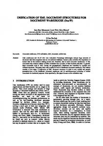
2. Motivations In this section, we highlight the relevance of structural and semantic similarity evaluation in XML comparison, using a bunch of motivating examples. We specifically focus on similarities left unaddressed in current XML comparison methods. 2.1. Structural Similarity XML documents can encompass many optional and repeated elements [36]. Such elements induce recurring sub-trees of similar or identical structures. As a result, algorithms for comparing XML document should be aware of such repetitions/resemblances so as to efficiently assess structural similarity. Consider, for example, dummy XML document trees A, B and C in Figure 1 (node labels stand for element/attribute names). One can realize that tree A is structurally more similar to B, than to C, the sub-tree A1, made up of nodes b, c and d, appearing twice in B (B1 and B2) and only once in C (C1). Nonetheless, such (sub-tree) structural similarities are left unaddressed by most existing approaches (even fine-grained ones such edit-distance methods), e.g. Chawathe’s method [10] considered as a reference point for the latest edit distance algorithms [13], [36]. In fact, Chawathe’s process permits applying changes to only one node at a time (using node insert, delete and update operations, with unit costs), thus yielding the same structural similarity value while comparing trees A/B and A/C. In theory, structural resemblances such as those between trees A/B and A/C could be taken into consideration by applying generalizations of Chawathe’s approach [10], developed in [36] (introducing edit operations allowing the insertion and deletion of whole sub-trees). Yet, our examination of the approaches provided in [13], [36] led us to identify certain cases where sub-tree structural similarities are disregarded. − Similarity between trees A/D (sub-trees A1 and D2) in comparison with A/E. − Similarity between trees F/G (sub-trees F1 and G2) relatively to F/H. − Similarity between trees F/I (sub-tree F1 and tree I) in comparison with F/J. The A, D, E case is special in that the XML document sub-trees being repeated are not identical to the source sub-tree, but are similar (e.g. D2 and A1 are similar not identical). Other types of sub-tree structural similarities that are missed by [36]’s approach (and likewise missed by [10], [13]) can also be identified when comparing trees F/G and F/H, as well as F/I and F/J. The F, G, H case is different than its predecessor (the A, D, E case) in that the sub-trees sharing structural similarities (F1 and G2) occur at different depths (whereas with A/D, A1 and D2 are at the same depth). On the other hand, the F, I, J case differs from the previous ones since structural similarities occur, not only among sub-trees, but also at the sub-tree/tree level (e.g., between sub-tree F1 and tree I). In addition, none of the approaches mentioned above is able to effectively compare documents made of repeating leaf node sub-trees. For example, following [10], [13], [36], identical similarity values are obtained when comparing document K, of Figure 1, to documents L and M. Nonetheless, one can realize that document trees K and L are more similar than K and M, node b of tree K appearing twice in tree L, and only once in XML tree M. Likewise for K/N with respect to K/P. Identical distances are attained when comparing document trees K/N and K/P, despite the fact that the node b is repeated three times in tree N, and only once in tree P.

Elsevier Science

4

In this study, we explicitly mention the case of leaf node repetitions since: − − −

Leaf nodes are a special kind of sub-trees: single node sub-trees. Therefore, the study of sub-tree resemblances and repetitions should logically cover leaf nodes, so as to attain a more complete XML similarity approach. Since leaf nodes come down to sub-trees, their repetitions might be as frequent as those of substructure repetitions (i.e. non-leaf node sub-tree repetitions) in XML documents. Detecting leaf node repetitions is spontaneous in the XML context, and would help increase the discriminative power of XML comparison methods, as shown in the above examples (which will be detailed subsequently). Tree A

a b

b

c

A1

d

c

B1

d

c

c

b

Tree J

h

c

j

a b

Tree K

d

b

f

h

d

g

h E2 Tree H

a H1

m

G2

H2

g

f

h Tree M

a b

b

Tree E e

Tree G

Tree L

a

c E1

m

G1

C2 a

h D2

g

f

d

b d

a

d

i

c

h

d

Tree I

b c

D1

c

C1

B2

b

b e

d

e

Tree D

a

b

b

c

d

Tree C

a

b

a Tree F

F1

Tree B

a

c

a b

b

i

j

Tree N b

a b

c

Tree P d

Fig. 1. Dummy XML trees.

2.2. Semantic Similarity In order to stress the need for semantic relatedness assessment in XML document comparison, we report from [48] the examples in Figure 2. Tree X

Tree Y

Tree Z

Academy

College

Factory

Division

Division

Division

Branch

Branch

Branch

Lecturer

Supervisor

Professor

Student

Fig. 2. Sample XML document trees.

Elsevier Science

5

Using classical edit distance computations (e.g. [10], [13], [36]), the same structural similarity value is obtained when document X is compared to documents Y and Z. However, despite having similar structural characteristics, one can easily recognize that sample document X shares more semantic characteristics with document Y than with Z. For instance, labels Academy-College and Professor-Lecturer, from documents X and Y, are commonly viewed as semantically more similar than Academy-Factory and Professor-Supervisor, from documents X and Z (considering a domain independent knowledge base such as WordNet2, describing concepts found in everyday language, cf. Section 3.3). Therefore, taking into account the semantic factor in XML similarity computations would obviously amend similarity results. As a matter of fact, such relatively simple semantic similarities have been covered in [48]. The authors in [48] complement Chawathe’s tree edit distance algorithm [10] with a ‘semantic cost scheme’ taking into account semantic similarities between XML node labels. They make use of a semantic similarity measure developed in [29], provided a given reference taxonomy. Tree B’

Tree C’

Institution

B’1

Academy

Professor

College

PhD Student

Tree A’

Institution

Lecturer

Scholar

C’1

Academy

Professor

H’1

Branch PhD Student

G’2

College

Lecturer

Scholar

Branch

H’2

Factory

Supervisor

Worker

Tree I’

Tree J’

College

Factory

Lecturer

Worker

Institution

G’1

Academy

Supervisor

C’2

Tree H’

Institution

A’1

Factory

PhD Student

Tree G’

Institution

Professor

B’2

Scholar

Supervisor

Worker

Tree L’

Tree M’

Institution

Institution

Tree K’ Institution

Professor

Professor

Professor

Lecturer

Professor

Supervisor

Tree N’

Tree P’

Institution

Institution

Lecturer

PhD Student

Professor

Supervisor

Worker

Fig. 3. Sample XML document trees with sub-tree semantic similarities.

——— 2 WordNet is a domain independent online lexical reference system, developed at Princeton University NJ USA, in an attempt to model the lexical knowledge of a native English speaker. It organizes nouns, verbs, adjectives and adverbs into synonym sets, each representing an underlying lexical concept [33] (http://www.cogsi.princeton.edu/cgi-bin/webwn).

6

Elsevier Science

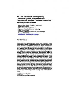
Nonetheless, as shown in Section 2.1, the approach in [10] was not designed to capture sub-tree repetitions and resemblances (making use of node-based edit operations). The same goes for its extension in [48] when comparing XML documents with semantically similar sub-trees. Consider for instance the sample XML document trees in Figure 3. Recall the A, B, C and A, D, E comparison cases in Figure 1, where A/B (likewise A/D) were structurally more similar than A/C (respectively A/E) due to the structural similarity (repetition) between sub-tree A1 and sub-tree B2 (likewise D2) in tree B (D). Here, document trees A’, B’ and C’ underline a similar scenario. While A’/B’ and A’/C’ are structurally indistinguishable, one can realize that A’ is semantically more similar to B’, than to C’. Sub-tree A’1 made of nodes Academy, Professor and PhD Student is semantically similar to sub-tree B’2 (made of nodes College, Lecturer and Scholar) in tree B’, while it is semantically different than sub-tree C’2 (of nodes Factory, Supervisor and Worker) in tree C’. In other words, instead of only considering the repetition of identical or structurally similar sub-tree patterns (as discussed in the Section 2.1), there is a need to consider the repetition of sub-trees that are semantically similar as well. Such (sub-tree) semantic similarities are left unaddressed by existing approaches, including that in [48], which only target single node semantic similarities. As with the sub-tree structural similarity examples in Figures 1, similar types of sub-tree semantic similarities can be identified when comparing trees A’/G’ and A’/H’, A’/I’ and A’/J’, K’/L’ and K’/M’, as well as K’/N’ and K’/P’. The A’, G’, H’ case is different in that the sub-trees sharing semantic similarities (A’1 and G’2) occur at different depths. The A’, I’, J’ case differs from its predecessors in that semantic similarities occur, not only among sub-trees, but also at the sub-tree/tree level (e.g., between sub-tree A’1 and tree I). On the other hand, the K’, L’, M’ and K’, N’, P’ cases correspond to leaf node semantic similarities. Here, one can realize that document trees K’ and L’ are more similar than K’ and M’, node Professor of tree K’ being semantically more similar to node Lecturer in tree L’, than to node Supervisor in tree M’. Likewise for K’/N’ with respect to K’/P’ (node Professor in K’ is semantically similar to Lecturer and PhD Student in tree N’ while it is relatively different than nodes Supervisor and Worker in tree P’). In short, we view the problem of XML document comparison as that of detecting the occurrences and repetitions of structurally/semantically similar sub-trees. In sub-trees, we underline multiple node as well as leaf node structures. Thus, we aim to provide a unified and fine-grained method to deal with both structural and semantic resemblances left addressed by existing XML comparison methods. 3. Preliminaries 3.1. XML Data Model XML documents represent hierarchically structured information and can be modeled as Ordered Labeled Trees (OLTs) [56]. In our study, each XML document is represented as an OLT with a node corresponding to each XML element and attribute. In fact, a traditional DOM (Document Object Model) ordered labeled tree is chiefly made of XML elements nodes, labeled with corresponding element tag names. Attributes mark the nodes of their containing elements. However, to incorporate attributes in their similarity computations, some approaches [36], [59] have considered OLTs with distinct attribute nodes, labeled with corresponding attribute names. Attribute nodes appear as children of their encompassing element nodes, sorted by attribute name, and appearing before all sub-element siblings [36]. The authors in [16], [36] disregard element/attribute values while studying the structural properties of heterogeneous XML documents. Note that other types of nodes, such as entities, comments and notations are also incorporated in the DOM model. Nonetheless, they are disregarded in most XML comparison approaches, e.g. [12], [13], [16], [36], …, since they underline complementary information and are not part of the core XML data. Definition 1 - Ordered labeled tree: it is a rooted tree in which the nodes are ordered and labeled (recall that node values are not considered in our XML tree model, only labels, i.e., XML element/attribute tag names). We denote by λ(T) the label of the root node of tree T. In the rest of this paper, the term tree means rooted ordered labeled tree ●

Elsevier Science

7

Definition 2 – Tree “Contained in” relationship: a tree A is said to be contained in a tree T if all nodes of A occur in T, with the same parent/child edge relationship and node order. Additional nodes may occur in T between nodes in the embedding of A (e.g., tree K is contained in tree A of Figure 1) ● Definition 3 - Sub-tree: given two trees T and T’, T’ is a sub-tree of T if all nodes of T’ occur in T, with the same parent/child edge relationship and node order, such as no additional nodes occur in the embedding of T’ (e.g., A1 in Figure 1 is a sub-tree of A, whereas tree K does not qualify as a sub-tree of A since nodes c and d occur in its embedding in A) ● Definition 4 - First level sub-tree: given a tree T with root p of degree k, the first level sub-trees, T1, …, Tk of T are the sub-trees rooted at the children nodes of p: p1, …, pk ● Definition 5 - Ld-pair representation of a node: it is defined as the pair (l, d) where l and d are respectively the node’s label and depth in the tree. We use p.l and p.d to refer to the label and the depth of an ld-pair node p respectively. Recall that node values are not considered in our XML tree model ● Definition 6 - Ld-pair representation of a tree: it is the list, in preorder, of the ld-pairs of its nodes (cf. Figure 4). Given a tree in ld-pair representation T = (t1, t2, …, tn), T[i] refers to the ith node ti of T. Thus, T[i].l and T[i].d denote, respectively, the label and the depth of the ith node of T, i designating the preorder traversal rank of node T[i] in T ● A1 = ((b, 0), (c, 1), (d, 1)) A11 = (c, 0) A12 = (d, 1) B1 = ((b, 0), (c, 1), (d, 1)) B11 = (c, 0) B12 = (d, 0) B2 = ((b, 0), (c, 1), (d, 1)) B21 = (c, 0) B22 = (d, 0) C1 = ((b, 0), (c, 1), (d, 1)) C11 = (c, 0) C12 = (d, 0) C2 = ((e, 0), (f, 1), (g, 1)) C21 = (f, 0) C22 = (g, 0)

D1 = ((b, 0), (c, 1), (d, 1), (h, 1)) D11 = (c, 0) D12 = (d, 0) D13 = (h, 0) D2 = ((b, 0), (c, 1), (d, 1), (h, 1)) D21 = (c, 0) D22 = (d, 0) D23 = (h, 0) E1 = ((b, 0), (c, 1), (d, 1), (h, 1)) E11 = (c , 0) E12 = (d, 0) E13 = (h, 0) E2 = ((e, 0), (f, 1), (g, 1), (h, 1)) E21 = (f, 0) E22 = (g, 0) E23 = (h, 0)

F1 = ((b, 0), (c, 1), (d, 1), (e, 1)) F11 = (c, 0) F12 = (d, 0) F13 = (e, 0) G1 = ((m, 0), (b, 1), (c, 2), (d, 2), (f, 2)) G2 = ((b, 0), (c, 1), (d, 1), (ef 1)) G21 = (c, 0) G22 = (d, 0) G23 = (f, 0) H1 = ((m, 0), (g, 1), (h, 2), (i, 2), (j, 2)) H2 = ((g, 0), (h, 1), (i, 1), (j, 1)) H21 = (h, 0) H22 = (i, 0) H23 = (j, 0) I1 = (c, 0) I2 = (d, 0) J1 = (i, 0) J2 = (j, 0)

Fig. 4. Ld-pair representations of all sub-trees in Figure 1, including single leaf node sub-trees.

3.2. Structural Similarity and Tree Edit Distance Methods for evaluating the structural similarity between semi-structured data, e.g., XML documents, generally exploit the dynamic programming techniques for finding the edit distance between trees, XML documents being modeled as OLTs. Hereunder, we provide basic notions and definitions describing the concept of tree edit distance. The background and detailed history of tree edit distance algorithms are reported to Section 7. Basically, the edit distance between two trees A and B is defined as the minimum cost edit script that transforms A to B: Dist(A, B) = Min{CostES }. An edit script is a sequence of edit operations op1, op2, …, opk, that is applied to a tree T, and that yields a tree T’ by executing each of its individual edit operations, following their order of appearance. By associating a cost, CostOp, to each edit operation in ES, the cost of ES can be computed as the sum of the costs of its component operations: CostES = ∑ |ES | CostOp . i=1

i

Thus, the problem of comparing two trees A and B, i.e. evaluating the structural similarity between A and B, is defined as the problem of computing the corresponding tree edit distance, i.e. minimum cost ES [58]. As for tree edit operations, they can be classified in two groups: atomic tree edit operations and complex edit operations. An atomic edit operation on a tree (i.e. rooted ordered labeled tree) is either the deletion of an inner/leaf node, the insertion of an inner/leaf node, or the replacement (i.e. update) of a node by another one. A complex tree edit operation is a set of atomic tree edit operations, treated as one single operation. A complex tree edit operation is either the insertion of a whole tree as a sub-tree in another tree (which is actually a sequence of atomic node insertion operations), the deletion of a whole tree (which consists of a sequence of atomic node deletion operations), or moving a

8

Elsevier Science

sub-tree from one position into another in its containing tree (which is a sequence of atomic node insertion/deletion operations). In the following, we present the definitions for each of the tree edit operations utilized in our approach. Definition 7 – Insert node: given a node x of degree 0 (leaf node) and a tree T with root node p having first level subtrees T1, …, Tm, Ins(x, i, p, l) is a node insertion applied to T, inserting x as the ith child of p, thus yielding T’ with first level sub-trees T1, … , Ti-1, x, Ti+1, … , Tm+1, where l is the label of x ● Definition 8 – Delete node: given a leaf node x and a tree T with root node p, x being the ith child of p, Del(x, p) is a node deletion operation applied to T that yields T’ with first level sub-trees T1, … , Ti-1, Ti+1, … , Tm ● Definition 9 – Update node: given a node x in tree T, and a label l, Upd(x, l) is a node update operation applied to x resulting in T’ which is identical to T except that in T’, x bears l as its label. The update operation could be also formulated as follows: Upd(x, y) where y.l denotes the new label to be assumed by x ● Definition 10 – Insert tree: given a tree A and a tree T with root node p having first level sub-trees T1, …, Tm , InsTree(A, i, p) is a tree insertion applied to T, inserting A as the ith sub-tree of p, thus yielding T’ with first level subtrees T1, …, Ti-1, A, Ti+1, …, Tm+1 ● Definition 11 – Delete tree: given a tree A and a tree T with root node p, A being the ith sub-tree of p, DelTree(A, p) is a tree deletion operation applied to T that yields T’ with first level sub-trees T1, … , Ti-1, Ti+1, … , Tm ● 3.3. Semantic Similarity Measures of semantic similarity are of key importance in evaluating the effectiveness of Web search mechanisms in finding and ranking results [31]. In the fields of Natural Language Processing (NLP) and Information Retrieval (IR), knowledge bases (i.e., thesauri, taxonomies and/or ontologies) provide a framework for organizing words/expressions into a semantic space [23]. In such a framework, evaluating the semantic similarity between words/expressions comes down to comparing the underlying concepts in the semantic space. In the following sub-sections, we provide basic notions and definitions related to knowledge bases and semantic similarity. The history and background of semantic similarity methods are thoroughly covered in Section 7. 3.3.1. Knowledge Base (Semantic Network) The study of word/expression relationships, particularly semantic similarity, can be assessed in terms of the information sources utilized [23]. Some knowledge-free approaches to evaluate the resemblance between words have been proposed [11], [22]. These rely exclusively on corpus data where word relationships are derived from their cooccurrence in the corpus itself. However, with corpus-based statistical approaches, “true” understanding of words is virtually unobtainable [23]. As a matter of fact, evaluating word similarities, according to their statistical distribution in a corpus, often captures syntactic, stylistic or pragmatic factors instead of semantic meaning [39]. Thus, the need for a predefined semantic reference arises. In the last two decades, manually built knowledge bases, (such as WordNet [33], Roget’s thesaurus [57], ODP [31], …) have been explored as reference information sources for understanding semantic relations between concepts and evaluating semantic similarity. A knowledge base generally comes down to a semantic network with a set of concepts representing groups of words/expressions (or URLs such as with ODP), and a set of links connecting the concepts, representing semantic relations. Definition 12 – Semantic network: it can be formally represented as a 3-tuple SN=(C, E, R, f) where: − C is the set of concepts (synonym sets as in WordNet [33]). − E is the set of edges connecting the concepts, where E ⊆ Vc ×Vc . , , Ω, …} (described in the following paragraph), the − R is the set of semantic relations, R = { ≺ , , synonymous words/expressions being integrated in the concepts themselves. − f is a function designating the nature of edges in E, f:E → R (cf. Figure 5)●

Elsevier Science

9

Entity 260 = N, the total number of word occurrences in the considered text corpus

Person; Individual Enrollee 29

Adult 25

Student; Scholar 28

Professional 25

PhD Student 12

Educator 21

Lecturer 8

62 Leader

Abstraction 4

Superior 3

Worker 2

Group

Employee 1

Social Group

Supervisor 2

Academic 13 Professor 12

Unit

44

Structure 78

5

Building 2 Complex

4

Organization 4 Institution

2

81

Plant

Division

1

Branch

1

2

Establishment 17 Academy 8

College 9

Factory 1

Concept (Synonym Set) Hyponym/Hypernym relations

Fig. 5. A (weighted) taxonomy fragment extracted from WordNet. The numbers next to concepts represent pre-computed concept frequencies (weights) based on a sample text corpus (cf. Section 3.3.2) and are not part of the taxonomy itself. They will be exploited in subsequent paragraphs.

Hereunder, we state the most popular semantic relations employed in the literature [33], [40]: − Synonym (≡): Two words/expressions are synonymous if they are semantically identical, that is if the substitution of one for the other does not change the initial semantic meaning (e.g., car ≡ automobile). − Hyponym ( ≺ ): It can be identified as the subordination relation, and is generally known as the Is Kind of relation or simply IsA (e.g., Barge ≺ Boat). − Hypernym ( ): It can be identified as the super-ordination relation, basically the inverse of Hyponym, and is generally known as the Has Kind of relation or simply HasA (Boat Barge). − Meronym ( ): It can be identified as the part-whole relation, and is generally known as PartOf, also MemberOf, SubstanceOf, ComponentOf, etc. (e.g., Rudder (PartOf) Vessel). − Holonym ( ): It is basically the inverse of Meronym, and is generally identified as HasPart, also HasMember, HasSubstance, HasComponent, etc. For the sake of completeness, we also mention the antonym relation. − Antonym (Ω): The antonym of an expression is its negation (e.g., Rise Ω Fall). Note that the Hyponym/Hypernym and Meronym/Holonym relations, which are hierarchical, make up the major part of existing semantic networks, in particular WordNet [33][40]. The synonym relation is normally intra-node, each concept grouping a set of synonymous words/expressions. On the other hand, most existing semantic similarity methods disregard the antonym relation as well as the various types of cross relations (e.g., RelatedTo, Cause/Effect…) [6], probably be due their scarceness in current semantic networks. Hence, in our study, we exploit hierarchical

semantic networks, generally known as taxonomies. 3.3.2. Semantic Similarity Measures Methods for estimating semantic similarity between words/expressions in a semantic network can be classified as edge-based and node-based. Methods of the former group are straightforward and generally estimate similarity as the shortest path (in edges, edge weights, or nodes) between the two concepts being compared. Hereunder, a classical variant of the edge-based measures [37]: SimEdge(w1, w2) = SimEdge(c1, c2) = 2×MaxDepth – [MinLength(c1, c2)] − c1 and c2 are concepts, in the taxonomy, subsuming words (expressions) w1 and w2 respectively − MaxDepth is the maximum depth of the taxonomy considered − MinLength(c1, c2) is the shortest path between concepts c1 and c2

(1)

Elsevier Science

10

Nonetheless, with node-based approaches, the definition of similarity is more sophisticated and is estimated as the maximum amount of information content they share in common. In a taxonomy, this common information carrier can be identified as the most specific common ancestor (also known as Lowest Common Ancestor or LCA) that subsumes both concepts being compared [39]. For instance, in Figure 5, LCA(Lecturer, Professor) = Educator, whereas LCA(Lecturer, Supervisor) = Person. Definition 13 – Information content: In information theory, the information content of a concept or class c is quantified as the negative log likelihood –log p(c) where p(c) is the probability of encountering an instance of c [39] ● Definition 14 – Probability of a concept: It is generally quantified with respect to the frequency of occurrence of the words/expressions, subsumed by the corresponding concept, in a given corpus ● Slightly different mathematical formulations have been utilized to compute concept probabilities. Hereunder the basic formulation by Resnick [39]: Freq(c) p(c) = (2) N − Freq(c) = ∑ count(w): sum of the number of occurrences, of words w Є words(c) subsumed by c, in a given corpus, − N: total number of words encountered in the corpus Since in taxonomies, concepts subsume those lower in the hierarchy, Freq(c) and consequently p(c) would increase as one moves up the hierarchy (the occurrence of a word is counted for its corresponding concept, as well as the concept’s ancestors). Thus, following Definition 13, nodes higher in the hierarchy, which have higher probabilities, would be less informative (more abstract). If the taxonomy considered has a root node, then its probability would be equal to 1, its information content being 0. Hereunder a classical variation of the node-based semantic similarity measures [39]: SimNode(w1, w2) = SimNode(c1, c2) = –log p(c0) −

(3)

c0 is the most specific common ancestor of c1 and c2.

A detailed presentation of existing semantic similarity methods is provided in Section 7. In the following section, we show how to combine information retrieval (IR)-style semantic similarity assessment and edit distance (ED)-based structural similarity evaluation, in order to define a combined semantic/structural similarity measure for comparing XML documents.

4. Proposal Our XML comparison method consists of four main modules: i) an algorithm for identifying the Structural Commonality Between two Sub-trees (Struct-CBS), ii), a process for quantifying the Semantic Resemblance Between two Sub-trees (Sem-RBS), iii) an algorithm for computing the Tree edit distance Operations Costs (TOC), iv) and a Tree Edit Distance algorithm TED. In short, the TOC algorithm makes use of Struct-CBS and Sem-RBS to structurally and semantically compare all sub-trees in the XML documents being compared. The produced sub-tree similarity results are consequently exploited as edit operations costs, in an adapted version of [36]’s main edit distance algorithm, which we identify as TED (cf. Figure 12). Hence, the inputs to our XML comparison approach are as follows: − The XML document trees to be compared, − Parameter α enabling the user to assign more importance to the structural or semantic aspects of the XML documents being treated, − A reference semantic network SN to be utilized for semantic similarity evaluation, weighted using corpusbased frequencies. Consequently, the method outputs the similarity between the XML document trees being compared. Our method’s overall architecture is depicted in Figure 6.

Elsevier Science

Tree T1 Tree T2

TOC

TED

11

Sim(T1, T2)

Parameter α Weighted SN

Struct-CBS

Sem-RBS

Fig. 6. Simplified activity diagram of our combined XML similarity approach.

Note that Struct-CBS and Sem-RBS can be applied to whole trees. However, in our study, their use is coupled with sub-trees. In the remainder of this section, we detail each of the algorithms and processes mentioned above. In addition, we compare the efficiency of our method w.r.t. existing approaches and assess its properties regarding the formal definition of similarity. Consequently, we discuss its overall time and space complexity. 4.1. Structural Similarity between Sub-trees (Struct-CBS) As shown in Section 2, sub-tree structural similarities are usually left undetected in current XML comparison approaches. In [36], the authors were the first to address the issue and were able to detect certain basic sub-tree structural similarities using the tree contained in relation (cf. Definition 2). Following [36], a tree A may be inserted in T only if A is already contained in the source tree T. Similarly, a tree A may be deleted only if A is already contained in the destination tree T. Therefore, the approach in [36] captures the sub-tree structural similarities between XML trees A/B in Figure 1, transforming A to B in a single edit operation: (inserting sub-tree B2 in A, B2 occurring in A as A1), whereas transforming A to C would always need three consecutive insert operations (inserting nodes e, f and g). Dist(A, C) = 3, which is the cost of three consecutive insert operations introducing nodes e, f and g in tree A transforming it into C. Nonetheless, when the containment relation is not fulfilled, certain structural similarities are ignored. Consider, for instance, trees A and D in Figure 1. Since D2 is not contained in A, it is inserted via four edit operations instead of one (insert tree), while transforming A to D, ignoring the fact that part of D2 (sub-tree of nodes b, c, d) is identical to A1. Therefore, equal distances are obtained when comparing trees A/D and A/E, disregarding A/D’s structural resemblances: Dist(A, D) = Dist(A, E) = 5. Likewise for the remaining comparison examples in Figure 1. Here, in order to capture the various kinds of sub-tree structural similarities pinpointed in Section 2.1, we identify the need to replace the tree contained in relation making up a necessary condition for executing tree insertion and deletion operations in [36] by introducing the notion of structural commonality between two sub-trees. Definition 15 – Structural commonality between sub-trees: given two sub-trees A = (a1, …, am) and B = (b1, …, bn), the structural commonality between A and B, designated by StructCom(A, B), is a set of nodes N = {n1, …, np} such that ∀ ni ∈ N, ni occurs in A and B with the same label, depth and relative node order (in preorder traversal ranking). For 1 ≤ i ≤ p ; 1 ≤ r ≤ m ; 1 ≤ u ≤ n: (1) ni.l = ar.l = bu.l (2) ni.d = ar.d = bu.d (3) For any nj ∈ N / i ≤ j, ∃ as ∈ A and bv ∈ B such as: • nj.l = as.l = bv.l • nj.d = as.d = bv.d • r ≤ s, u ≤ v (4) There is no set of nodes N’ that satisfies conditions 1, 2 and 3 and is of larger cardinality than N ●

Elsevier Science

12

In other words, StructCom(A, B)3 identifies the set of matching nodes between sub-trees A and B, node matching being undertaken with respect to the node label, depth and relative preorder ranking. Algorithm Struct-CBS() Input: Sub-trees SbTi and SbTj (in ld-pair representations) Output: Normalized structural commonality between SbTi and SbTj Begin Dist [][] = new [0...|SbTi|][0…|SbTj|] Dist[0][0] = 0

1

For (n = 1 ; n ≤ |SbTi| ; n++) { Dist[n][0] = Dist[n-1][0] + CostDel(SbTi[n]) } For (m = 1 ; m ≤ |SbTj| ; m++) { Dist[0][m] = Dist[0][m-1] + CostIns(SbTj[m]) } For (n = 1 ; n ≤ |SbTi| ; n++) { For (m = 1 ; m ≤ |SbTj| ; m++) { Dist[n][m] = min{ If (SbTi[n].d = SbTj[m].d & SbTi[n].l = SbTj[m].l) { Dist[n-1][m-1] }, Dist[n-1][m] + CostDel(SbTi[n]), // simplified node // operations syntaxes. Dist[n][m-1] + CostIns(SbTj[m]) } } } Return

|SbTi |+|SbTj | - Dist[|SbTi |][|SbTj |]

5

10

15

20

// normalized commonality

2 Max(SbT , SbT ) i

j

End

Fig. 7. Algorithm Struct-CBS for identifying the structural commonality between sub-trees.

Following Definition 15, the problem of finding the structural commonality between two sub-trees SbTi and SbTj is equivalent to finding the maximum number of structurally matching nodes in SbTi and SbTj (|StructCom(SbTi, SbTj)|). However, the problem of finding the edit distance between SbTi and SbTj comes down to identifying the minimal number of edit operations that can transform SbTi to SbTj. Those are dual problems since identifying the edit distance between two sub-trees (trees) underscores, in a roundabout way, their maximum number of matching nodes (In other words, the greater the edit distance, the larger the edit script, the greater the number of edit operations, the greater the number of node transformations, the lesser the number of matching nodes). Therefore, we introduce in Figure 7 our Struct-CBS algorithm, based on the edit distance concept, to identify the structural commonality between sub-trees (similarly to the approach provided in [34] in which the author develops an edit distance based approach for computing the longest common sub-sequence between two strings). In Struct-CBS, sub-trees are treated in their ld-pair representations (cf. Definitions 5-6, Figure 4). Using the ldpair tree representations, sub-trees are transformed into modified sequences (ld-pairs), making them suitable for standard edit distance computations. Afterward, the maximum number of matching nodes between SbTi and SbTj, |StructCom (SbTi, SbTj)|, is identified with respect to the edit distance: − Total number of deletions - we delete all nodes of SbTi except those having matching nodes in SbTj: ∑ = |SbTi| - |StructCom(SbTi , SbTj)| Deletions

− Total number of insertions - we insert into SbTi all nodes of SbTj except those having matching nodes in SbTi: ∑ = |SbTj| - |StructCom(SbTi , SbTj)| Insertions

——— 3 Our sub-tree structural commonality definition can be equally applied to whole trees (a sub-tree being basically a tree). However, in this study, it is mostly utilized with sub-trees.

Elsevier Science

13

− Following Struct-CBS, using constant unit costs (=1) for node insertion and deletion operations, the edit distance between sub-trees SbTi and SbTj becomes as follows: Dist[|SbTi|][|SbTj|] =

∑

Deletions

°1+

∑

Insertions

− Therefore, |StructCom(SbTi , SbTj )| =

° 1 = |SbTi| + |SbTj| - 2 |StructCom(SbTi , SbTj)|

|SbTi |+|SbTj | - Dist[|SbTi |][|SbTj |]

(4)

2

To obtain structural commonality values comprised in the [0, 1] interval, we normalize |StructCom(SbTi, SbTj)| via corresponding sub-tree cardinalities Max(|SbTi|, |SbTj|). Thus: −

−

| StructCom (SbTi , SbTj )| Max(|SbTi | , |SbTj |) | StructCom (SbTi , SbTj )| Max(|SbTi | , |SbTj |)

=0

When there is no structural commonality between SbTi and SbTj : |StructCom(SbTi, SbTj)| = 0

=1

When the sub-trees are identical: |StructCom(SbTi, SbTj)| = |SbTi| = |SbTj|

Tables 1 and 2 show the detailed computations and results of applying Struct-CBS to sample sub-trees A1, D1, and C2, G2 of Figure 1. Tab. 1. Detailed edit distance computations, following Struct-CBS, when applied on sub-trees A1 and D1. 0 A1[1] (b, 0) A1[2] (c, 1) A1[3] (d, 1)

0 0 1 2 3

D1[1] (b, 0) 1 0 1 2

D1[2] (c, 1) 2 1 0 1

D1[3] (d, 1) 3 2 1 0

D1[4] (h, 1) 4 3 2 1

Note that the matching nodes are highlighted while the (final) distance value is emphasized in italic format. Having Dist[|A1|][|D2|] = 1: |A |+|D2 | - Dist[|A1 |][|D2 |] 3 + 4 -1 |StructCom (A1 , D2 )| = 1 = = 3 , (nodes b, c, d). 2 2 Consequently, the normalized value Struct-CBS(A1, D1) = 3/4 = 0.75 Tab. 2. Detailed edit distance computations, following Struct-CBS, when applied on sub-trees C2 and G2. 0 C2[1] (e, 0) C2[2] (f, 1) C2[3] (g, 1)

0 0 1 2 3

G2[1] (b, 0) 1 2 3 4

G2[2] (c, 1) 2 3 4 5

G2[3] (d, 1) 3 4 5 6

G2[4] (f, 1) 4 5 4 5

Having Dist[|C2|][|G2|] = 5: |StructCom (C2 , G2 )| =

|C 2 |+|G2 | - Dist [|C 2 |][|G2 |] 2

=

3+ 4-5 2

= 1 , (node f).

Thus, Struct-CBS(C2, G2) = 1/4 = 0.25 Note that applying Struct-CBS to leaf node sub-trees comes down to comparing two labels: those of the leaf nodes at hand. For example: − Struct-CBS(A11, B11) = 1, A11 and B11 consisting of leaf node c, − Sruct-CBS(A11, B12) = 0, A11 and B12 having different labels (λ(A11) = A11[0].l= c whereas λ(B12) = d).

Elsevier Science

14

Similarly, when computing the commonality between a leaf node sub-tree (e.g., A11) and a non-leaf node subtree (e.g., B1), Struct-CBS compares the label of the former (λ(A11)) to the label of the root node of the latter (λ(B1)): − For example, Struct-CBS(A11, B1) = 0, A11 and the root of B11 having different labels (λ(A11) = A11[0].l = c whereas λ(B1) = B1 [0].l = b). − Struct-CBS(E22, H2) = 1/4 = 0.25 having |StructCom(E22, H2)| = 1 (λ(E22) = λ(H2) = g) and Max(|E22|, H2|) = 4. We do not present detailed Struct-CBS results, when leaf node sub-trees are considered in the computation process, due to their intuitiveness. 4.2. Semantic Resemblance between Sub-trees (Sem-RBS) In addition to sub-tree structural commonalities, we aim to consider sub-tree semantics in XML similarity evaluation. In Section 2.2, we have presented a bunch of motivation examples underlining the need to capture the semantic resemblances between sub-trees while comparing XML documents. Note that for the sake of clearness, we use the expression ‘semantic resemblance’ between sub-trees, in the remainder of the paper, to avoid any confusion between semantic and structural similarity, the latter being designated as ‘structural commonality’. Various methods for detecting the semantic similarity between pairs of words/expressions, based on a given reference semantic network, have been proposed (cf. Section 7.2). Nonetheless, capturing the semantic relatedness between two groups of words/expressions (e.g., node labels of two sub-trees) is left unaddressed, to the exception of a few theoretical yet unpractical studies, which we cover in Section 6. To capture the semantic resemblance between two sub-trees, we combine the traditional vector space model in information retrieval [32] with classic semantic similarity assessment (cf. Section 3.3). In detail, we proceed as follows. When comparing two sub-trees SbTi and SbTj, each sub-tree would be represented as a vector V (Vi and Vj respectively) with weights underlining the semantic similarities between each of their corresponding node labels. Definition 16 – Sub-tree vector space: For two sub-trees SbTi and SbTj, vectors Vi and Vj are produced in a space which dimensions represent, each, a distinct indexing unit. An indexing unit stands for a single node label lr ∈ SbTi U SbTj, such as 1 < r < n where n is the number of distinct node labels in both SbTi and SbTj. The coordinate of a given sub-tree vector Vi on dimension lr is noted wVi(lr) and stands for the semantic weight of lr in sub-tree SbTi ● Definition 17 – Semantic node label weight: The semantic weight of a node label lr in sub-tree SbTi of vector Vi is composed of two factors: a node/vector similarity factor Sim(vr, Vi, SN) and a depth D-factor(vr) factor, such as wVi(lr)= Sim(vr, Vi, SN) ×D-factor(vr) ∈ [0, 1]. − Sim(vr, Vi, SN) quantifies the semantic similarity between label lr of node vr and sub-tree vector Vi. It is computed as the maximum semantic similarity between lr and all node labels of SbTi with respect to a reference semantic network SN. Formally, Sim(vr , Vi , SN)= Max ( Sim( vr , v, SN )) ∈ [0, 1]. Here, a classical v ∈ Vi

semantic similarity measure is exploited to compute pair-wise similarity values Sim(vr, v, SN) (Section 4.2.1). − D-factor underlines the semantic influence of node depth on XML semantic similarity. It follows the intuition that information placed near the root node of an XML document is more important than information further down in the hierarchy [4], [59]. Thus, node labels higher in the XML tree hierarchy should have a greater semantic influence than their lower counterparts. This could be mathematically concretized using formula 5, adapted from [59].

D-factor (p.l)=

1 ∈ [0, 1] 1 + p.d

where p.l and p.d are respectively the label and depth of node p ●

(5)

Hence, having transformed sub-trees into semantically weighted vectors, the semantic relatedness between two sub-trees can be evaluated using a measure of similarity between vectors such as the inner product, the cosine measure, the Jaccard measure, etc. Here, we adopt the cosine measure widely exploited in information retrieval [5], [42]: n

Sem -RBS (SbTi , SbT j , KB ) = Cos(Vi , V j ) =

∑ w SbTi (l r ) × w SbTj (l r )

r=1 n

2

n

∑ w SbTi (lr ) × ∑ w SbTj (lr )

r =1

r =1

2

∈ [0, 1]

(6)

Elsevier Science

15

Algorithm Sem-RBS() Input: Sub-trees SbTi and SbTj (in ld-pair), weighted semantic network SN Output: Semantic resemblance between SbTi and SbTj

Begin

1

VS = Generate_Vector_Space(SbTi, SbTj) Vi = Generate_Occurrence_Vector(SbTi, VS) Vj = Generate_Occurrence_Vector(SbTj, VS)

// Vectors with simple node // occurrence weights: 0/non null, // taking into account node depths // Computing semantic weights for vector Vi

5 For each node label lr in Vi { If (wVi(lr) == 0) { 10 For each node label ls in SbTi { SemWeight = SN-factor(lr, ls, SN) * D-factor(lr) // Semantic weight If (SemWeight > wVi(lr) ) { wVi(lr) = SemWeight } // Max } } 15 }

For each node label ls in Vj //Computing semantic weights for vector Vj { If (wVj(ls) == 0) { 20 For each node label lr in SbTj { SemWeight = SN-factor(ls, lr, SN) Χ D-factor(ls) // Semantic weight If (SemWeight > wVi(lr) ) { wVj(ls) = SemWeight } // Max } 25 } } ScalarProduct = 0 Modulei=0 Modulej=0

30

For each label lr in VS // Computing the cosine measure Cos(Vi, Vj) { ScalarProduct = Product + wVj(lr) * wVj(lr) Modulei = Modulei + wVj(lr)2 Modulej = Modulej + wVj(lr)2 } Product

Return

35

// Sem-RBS(SbTi, SbTj, SN) = Cos(Vi, Vj)

Modulei +Module j

Fig. 8. Algorithm Sem-RBS for evaluating the semantic resemblance between two sub-trees.

Algorithm Sem-RBS is shown in Figure 8. It simply consists of building the vector space corresponding to the sub-trees being compared as well as computing the semantic and cosine measures as explained above. On the other hand, we believe that Formula 6 is self explanatory in terms of the algorithm’s input parameters (sub-trees SbTi and SbTj to be compared, and the reference semantic network SN to be employed) as well as its output result (semantic similarity value comprised in the [0, 1] interval). 4.2.1. Semantic Similarity Measure As for the semantic similarity measure exploited to compute the SN-factor (cf. Definition 17), our investigation of the literature (cf. Section 7.2) led us to consider Lin’s method [29] in our XML comparison process. Lin’s measure was proven efficient in evaluating semantic similarity, in comparison with its predecessors, i.e. [39], [55]. Its performance and theoretical basis are recognized and generalized by [31] to deal with hierarchical and non-hierarchical structures. It is important to note that our XML similarity approach is not sensitive, in its definition, to the semantic similarity measure used. However, choosing a performing measure would yield better similarity judgment.

Elsevier Science

16

Following [29], the semantic similarity between two words (expressions) can be computed as follows: Sim Lin (w 1 , w 2 ) = Sim Lin (c1 , c 2 ) =

− − −

2 log p(c 0 ) ∈ [0,1] log p(c1 ) + log p(c 2 )

(7)

c1 and c2 are concepts, in a semantic network of hierarchical structure (taxonomy), subsuming words (expressions) w1 and w2 respectively c0 is the most specific common ancestor of concepts c1 and c2 p(c) denotes the occurrence probability of words corresponding to concept c (cf. Definition 14, Formula 2).

Recall that in information theory, the information content of a class or concept c is measured by the negative log likelihood -log p(c) (cf. Definition 13). While comparing two concepts c1 and c2, Lin’s measure [29] takes into account each concept’s information content (-log p(c1) + -log p(c2)), as well as the information content of their most specific common ancestor (-log p(c0)), in a way to increase with commonality (information content of c0) and decrease with difference (information content of c1 and c2). 4.2.2. Computation Examples Consider for instance sub-trees A’1, B’2 and C’2 of Figure 3. Detailed computations and results when comparing sub-trees A’1, B’2 and A’1, C’2 are shown below. When comparing A’1 and B’2, the corresponding vector space consists of 6 dimensions corresponding to each distinct node label in both sub-trees: Academy, Professor, PhD Student, College, Lecture and Scholar. Thus, 6dimensional vectors VA’1 and VB’2 are produced as shown in Figure 9.

VA’1 VB’2

Academy

Professor

PhD Student

College

Lecturer

Scholar

1 0

1 0

1 0

0 1

0 1

0 1 4

a. Simple node label occurrence vectors

VA’1 VB’2

Academy

Professor

PhD Student

College

Lecturer

Scholar

Academy

Professor

PhD Student

College

Lecturer

Scholar

1 0.7970

1 0.7674

1 0.8402

0.7970 1

0.7674 1

0.8402 1

1 0.7970

0.5 0.3838

0.5 0.4202

0.7970 1

0.3838 0.5

0.4202 0.5

b. SN-factor semantic values

c. Final weights, i.e. SN-factor × D-factor

Fig. 9. Sub-tree vectors obtained when comparing sub-trees A’1 and B’2

SN-factor values are computed following Lin’s semantic similarity measure [29] (cf. Formula 7). Here, in computing SN-factor values, we exploit a fragment of WordNet, along with pre-computed word occurrences based on a given text corpus (cf. Figure 5). Similarity values, following [29], between pairs Academy/College, Professor/Lecturer, and PhD Student/ Scholar are given below: Sim Lin (Academy, College) =

2 log p(Establishment ) log p(Academy ) + log p(College)

Sim Lin (Professor , Lecturer ) =

2 log ( = log (

2 log p(Educator ) log p(Professor ) + log p(Lecturer )

Sim Lin (PhD Student , Scholar ) =

8 260

17 260

)

) + log (

9 260

= 0.7970 )

= 0.7674

2 log p(Scholar ) log p(PhD Student ) + log p(Scholar )

= 0.8402

——— 4 We show the simple occurrence vectors to clarify the semantic vector construction process. Occurrence vectors are utilized in our implementation processes. Yet, from a theoretical point of view, we need not mention them and can directly compute semantic weights.

Elsevier Science

17

Recall that SN-factor underlines the semantic similarity between a label l and a vector V, and is computed as the maximum semantic similarity between l and all node labels of V (cf. Definition 17). In our example, SimLin(Laboratory, College) underlines the maximum similarity value between label Laboratory and all labels of vector VB’2, and viceversa for College and vector VA’1. The same is true for node labels Professor and Lecturer, as well as PhD Student and Scholar, w.r.t. vectors VB’2 and VA’1 respectively (cf. Figure 9.b). Consequently, final vector weights are obtained by multiplying both semantic network and depth factors SN-factor × D-factor as shown in Figure 9.c (cf. Definition 17). As a result, the semantic resemblance between sub-trees A’1 and B’2 is computed as follows: 2.3979

Sem -RBS (A'1 , B' 2 ) = Cos(VA' 1 , VB' 2 ) =

= 0.9752

2.4588

When comparing A’1 and C’2, the corresponding vector space also consists of 6 dimensions corresponding to each distinct node label in both sub-trees: Academy, Professor, PhD Student, Factory, Supervisor and Worker. Academy

Professor

PhD Student

Factory

Supervisor

Worker

1 0

1 0

1 0

0 1

0 1

0 1

VA’1 VC’2

a. Simple node label occurrence vectors

VA’1 VC’2

Academy

Professor

PhD Student

Factory

Supervisor

Worker

Academy

Professor

PhD Student

Factory

Supervisor

Worker

1 0.2662

1 0.3608

1 0.3608

0.2662 1

0.3608 1

0.3608 1

1 0.2662

0.5 0.1804

0.5 0.1804

0.2662 1

0.1804 0.5

0.1804 0.5

b. SN-factor semantic values

c. Semantic weights, i.e. SN-factor × D-factor

Fig. 10. Sub-tree vectors obtained when comparing sub-trees A’1 and C’2

Detailed semantic similarity computations, following [29], based on the taxonomy and word occurrences shown in Figure 10, are developed below (cf. Figure 10.b). Sim Lin (Academy, Factory ) =

2 log p(Structure) log p(Academy ) + log p(Factory )

Sim Lin (Professor , Supervisor )=

2 log p( = log p(

2 log p(Person ) log p(Professor ) + log p(Supervisor )

Sim Lin (PhD Student , Worker ) =

2 log p(Person) log p(PhD Student ) + log p(Worker )

8 260

78 260

)

) + log p(

1 260

= 0.2662 )

= 0.3608

= 0.3608

Consequently, the semantic resemblance between sub-trees A’1 and C’2 would be computed as follows: Sem -RBS (A'1 , C' 2 ) = Cos(VA' 1 , VC' 2 ) =

0.8935

= 0.5461

1.6361

Results show that sub-tree A’1 (made of node labels Academy, Professor and PhD Student) is semantically more similar to sub-tree B’2 (College, Lecturer, Scholar) than C’2 (Factory, Supervisor, Worker). 4.3. Tree Edit Operations Costs (TOC) As stated previously, TOC is an algorithm dedicated to computing tree edit distance operations costs, based on sub-tree structural commonalities (Struct-CBS) and semantic resemblances (Sem-RBS). Consequently, the costs will be exploited via an adaptation of Nierman and Jagadish’s main edit distance algorithm [36] (cf. Figure 12) providing an improved and more accurate XML similarity measure.

Elsevier Science

18

TOC, developed in Figure 11, consists of three main steps: − Step 1 (lines 2-13) identifies the structural commonalities and semantic resemblances between each pair of sub-trees in the source and destination trees respectively (T1 and T2), assigning tree insert/delete operation costs accordingly. − Step 2 (lines 14-18) identifies the structural commonalities and semantic resemblances between each subtree in the source tree (T1) and the destination tree (T2) as a whole, updating delete tree operation costs correspondingly. − Step 3 (lines 19-24) identifies the structural commonalities and semantic resemblances between each subtree in the destination tree (T2) and the source tree (T1) as a whole, modifying insert tree operation costs accordingly. Algorithm TOC() Input: Trees T1, T2, parameter α for weighting Struct-CBS and Sem-RBS, weighted semantic network SN Output: Insert tree and delete tree operations costs

Begin

1

For each sub-tree SbTi in T1 { CostDelTree(SbTi) =

∑

// Going through // all sub-trees of T1

Cost

( x)

Del All nodes x of SbTi

For each sub-tree SbTj in T2 { CostInsTree(SbTj) =

∑

Cost

// Going through // all sub-trees of T2

5

( x)

Ins All nodes x of SbT j

CostDelTree(SbTi) = Min{ CostDelTree(SbTi),

∑ CostDel ( x ) × All nodes x of SbTi

1 1+ α Struct-CBS(SbTi , SbTj ) + (1- α )Sem-RBS(SbTi , SbTj , KB)

}

CostInsTree(SbTj) = Min{ CostInsTree(SbTj),

∑ CostIns ( x) × All nodes x of SbTj

10

1 1+ α Struct-CBS(SbTi , SbTj ) + (1-α ) Sem-RBS(SbTi , SbTj , KB)

}

} } For each sub-tree SbTi in T1 // Comparing sub-trees in T1 { // to whole tree T2. CostDelTree(SbTi) = Min{ CostDelTree(SbTi),

∑ CostDel ( x) × All nodes x of SbTi

15

1 1+ α Struct-CBS(SbTi , T2 ) + (1-α ) Sem-RBS(SbTi , T2 , KB)

}

} For each sub-tree SbTj in T2 { CostInsTree(SbTj) = Min{ CostInsTree(SbTj),

∑ CostIns ( x) × All nodes x of SbTj

// Comparing sub-trees in T2 // to whole tree T1.

20

1 1+ α Struct-CBS(T1 , SbTj ) + (1-α ) Sem-RBS(T1 , SbTj , KB)

}

} End

25

Fig. 11. Tree edit distance Operations Costs (TOC) algorithm.

Elsevier Science

19

Steps 2 and 3 are introduced to capture, not only the structural/semantic similarities between sub-trees, but also the similarities between the sub-trees and the overall trees being compared. The relevance of steps 2 and 3 becomes obvious when one of the trees involved in the comparison process shares structural/semantic similarities with one (or more) of the sub-trees encompassed in the other XML document tree. Note for instance: − The F, I, J case in Figure 1, where tree I is structurally similar to sub-tree F1 of tree F − The A’, I’, J’ case in Figure 3 where tree I’ is semantically similar to sub-tree A’1 of tree A. Using Struct-CBS and Sem-RBS, the TOC algorithm identifies the structural commonalities and semantic resemblances between each and every pair of sub-trees (SbTi, SbTj) in the two trees T1 and T2 being compared (step 1), as well as their similarities with the whole trees T1 and T2 respectively (steps 2 and 3).

Following TOC, tree operations costs vary as follows: CostInsTree/DelTree(SbTi) = ∑ Cost Ins/Del ( x ) ×

1

All nodes x of SbTi

1 + α Struct -CBS(SbTi , SbTj ) + (1-α ) Sem-RBS(SbTi , SbTj )

where

provided as user input

α ∈ [0, 1] is

Maximum insert/delete tree cost for sub-tree Sbi:

CostInsTree/DelTree(SbTi) = ∑ Cost Ins/Del ( x ) × 1 All nodes x of SbTi

(8)

Minimum insert/delete tree cost for sub-tree Sbi:

CostInsTree/DelTree(SbTi) = ∑ Cost Ins/Del ( x ) × All nodes x of SbTi

1 2

Lemma 1. Following TOC, the maximal insert/delete tree operation cost for a given sub-tree SbTi (attained when no sub-tree structural commonalities nor semantic resemblances with SbTi are identified in the source/destination tree respectively) is the sum of the costs (unit costs, =1)5 of inserting/deleting every individual node of SbTi (the proof is evident). Lemma 2. Following TOC, the minimal insert/delete tree operation cost for SbTi (attained when a sub-tree identical to SbTi is identified in the source/destination tree respectively) is equal to half its corresponding insert/delete tree maximum cost. The minimal tree operation cost is defined in such a way in order to guarantee that the cost of inserting/deleting a non-leaf node sub-tree will never be less than the cost of inserting/deleting a single node (single node operations having unit costs). In fact, TOC is based on the intuition that tree operations are more costly than node operations. Proof: The smallest non-leaf node sub-tree that can be treated via a tree operation is a sub-tree consisting of two nodes. For such a tree, the minimum insert/delete tree operation cost would be equal to 1 (its maximum cost being equal to 2), equivalent to the cost of inserting/deleting a single node. That is the lowest tree operation cost attainable, for a non-leaf node sub-tree, following TOC. Hence, for leaf node sub-trees, the maximum insert/delete tree operation cost is equal to 1, the cost of inserting/deleting the single node at hand: − CostInsTree/DelTree(SbTi) = CostIns/Del(x) × 1= 1 , that is when SbTi is made of single node x The minimum cost for inserting/deleting a single node sub-tree is equal to 0.5, half its maximum insertion/deletion cost: − CostInsTree/DelTree(SbTi) = CostIns/Del(x) × 1/2 = 0.5 , SbTi consisting of single node x Note that in our approach, single node insertions/deletions are undertaken via tree insert/delete operations (cf. Definitions 10 and 11) applied on leaf node sub-trees. On the other hand, insert/delete node operations (cf. Definitions 7 and 8, which are assigned unit costs as with traditional edit distance approaches) are only utilized to compute tree ——— 5 An intuitive and natural way has been usually used to assign single node operation costs and consists of considering identical unit costs for insertion and deletion operations [9][36].

Elsevier Science

20

insertion/deletion operations costs (cf. Struct-CBS in Figure 7 and TOC in Figure 11 - lines 4 and 7). They do not however contribute to the dynamic programming procedure adopted in our edit distance approach (similarly to [13][36], cf. TED algorithm in Figure 12). Thus, using TOC, we compute the costs of tree insertion and deletion operations based on their corresponding trees’ structural commonality and semantic resemblance values (maximum structural commonality/semantic resemblance values inducing minimum tree operations costs). In addition, TOC (and thus the overall approach) enables the user to assign more importance to either structural or semantic similarities by varying parameter α ∈ [0, 1]: − For α= 1, TOC will only consider structural commonalities in computing operations costs (via Struct-CBS). − For α = 0, only sub-tree semantic resemblances will be considered in computing operations costs (Sem-RBS). Providing such a capability would enable the user, as stated previously in the paper, to parameterize and adapt the XML comparison process following the scenario at hand, stressing on the structural or (inclusive) semantic aspects of the XML documents being compared. Recall that utilizing the contained in relation introduced in [36] (cf. Definition 2) in order to permit or deny tree insertion/deletion operations is not effective since it disregards certain sub-tree structural similarities while comparing two XML trees (as shown in Section 2.1). As a result, our method permits the insertion and deletion of any/all sub-trees by varying their corresponding tree insertion/deletion operation costs with respect to their structural commonalities with the source/destination trees/sub-trees respectively. In addition, our approach takes into account XML tree/sub-tree semantics, by varying edit operations costs accordingly. The weights of structural and semantic sub-tree similarities on tree operations costs, and consequently on the overall approach, are chosen following the user’s needs (she might want to completely disregard semantics and only focus on XML structure in a given scenario, or focus on semantics, …). Note that inserting/deleting the whole destination/source trees is not allowed in our approach (cf. Algorithm TED). In fact, by allowing such operations, one could delete the entire source tree in one step and insert the entire destination tree in a second step, which completely undermines the purpose of the insert/delete tree operations. 4.4. Tree Edit Distance (TED) The tree edit distance algorithm TED, utilized in our study, is developed in Figure 12. It is an adaptation of Nierman and Jagadish’s main edit distance process [36]. In addition to tree insertion/deletion operations costs which vary w.r.t. the structural/semantic similarities between XML sub-trees, TED exploits update operations costs (cf. Figure 12 line 5) in computing the distance between two XML document trees. Using the update operation, the edit distance algorithm compares the roots of the sub-trees actually considered in the recursive process (at startup, these would correspond to the roots of the XML trees being compared). With classical edit distance approaches, the cost of an update operation underlines the equality/difference between the concerned node labels: − Minimum cost when the compared element labels are identical, CostUpd(a, b) = 0 when a.l = b.l − Maximum unit cost otherwise, i.e. CostUpd(a, b) = 1 when a.l ≠ b.l Nonetheless, to consider the semantic similarities between element labels (not only label equality/difference) in our study, we extend the update operation cost scheme as follows: ⎡ ⎢(1 - (1-α ) ( Sim (a.l, b.l, SN)) ×

Cost Upd (a, b) = ⎢ ⎢⎣

0 otherwise

⎤ α + D -fact (a.d) if a.l ≠ b.l ⎥ 1 + α D -fact (a.d) ⎥ ⎥⎦

where α ∈ [0, 1]

(9)

Parameter α is the same utilized in TOC to assign more importance to structural or semantic similarities: − For α = 1, we will only consider label equality/difference in computing the cost of the update operation, as with traditional structural edit distance approaches, − For α = 0, node semantic similarities will be considered in computing the update operation cost. Here, update operations costs would vary in the [0, 1] interval w.r.t. to the semantic similarity between the concerned node labels and corresponding depths (note that nodes being treated via the update operation are always of the same depth, i.e. a.d = b.d).

Elsevier Science

21

Algorithm TED() Input: Trees A and B, deletion/insertion operations costs CostDelTree/CostInsTree for all sub-trees in trees A/B respectively, parameter α for structural/semantic weighting, weighted semantic network SN Output: Edit distance between A and B

Begin M = Degree(A) N = Degree(B)

1 // The number of first level sub-trees in A. // The number of first level sub-trees in B.

Dist [][] = new [0...M][0…N] Dist[0][0] = CostUpd(λ(A), λ(B), α, SN)

//Update operation

For (i = 1 ; i ≤ M ; i++) { Dist[i][0] = Dist[i-1][0] + CostDelTree(Ai) } For (j = 1 ; j ≤ N ; j++) { Dist[0][j] = Dist[0][j-1] + CostInsTree(Bj) } For (i = 1 ; i ≤ M ; i++) { For (j = 1 ; j ≤ N ; j++) { Dist[i][j] = min{ //Dynamic Dist[i-1][j-1] + TED(Ai, Bj), //programming Dist[i-1][j] + CostDelTree(Ai), Dist[i][j-1] + CostInsTree(Bj) } } } Return Dist[M][N]

5

10

15

// Sim = 1 / (1+ Dist)

End

20

Fig. 12. Edit distance algorithm TED.

Consider for instance document trees X, Y and Z in Figure 2. With α= 0, the corresponding root update operations costs would be as follows: − CostUpd(λ(X), λ(Y)) = 1 – ( SimLin(Academy, College) × 1) = 0.2030 − CostUpd(λ(X), λ(Z)) = 1 – ( SimLin(Academy, Factory) × 1) = 0.7337 It is clear that the cost of updating Academy and College is lesser than that of transforming Academy into Factory, identifying the fact that the former couple is more semantically similar, following the taxonomy in Figure 5, than the latter (Detailed computation examples are developed in the following section). Here, as with Sem-RBS, we exploit Lin’s measure [29] to assess the semantic similarity between node labels (i.e., in computing the SN-factor). However, recall that its use is not mandatory. We use it since it is among the most efficient measures available, as discussed previously. 4.5. Computation Examples In the following, we present two detailed computation examples. The first shows how our approach considers structural commonalities in comparing XML trees. The second focuses on semantic resemblances between sub-trees. Similarity results for all XML motivation examples mentioned in Section 2 are reported and discussed subsequently. 4.5.1. Structural Similarity Evaluation In this example, we consider the case of dummy XML document trees A, D and E in Figure 1. Recall that trees D and E are considered identical with respect to A following current approaches, i.e. [10], [13], [36], despite the fact that A/D share more structural similarities than A/E (as discussed in Section 2.1.1). In order to compare trees A/D, we start by executing algorithm TOC which yields the following insertion/deletion operations costs. Note that in this example, parameter α is set to 1 since we only focus on XML structural commonalities. In fact, node labels in trees A, D and E are made of simple characters and have no semantic meanings. Thus, it would be useless to consider Sem-RBS in this case, which would obviously return null results.

Elsevier Science

22

When applied to XML trees A and D, with α =1, our approach yields Dist(A, D) = 3.2856 (cf. Table 3) having: CostUpd(λ(A), λ(D)) = 0, where λ(A).l = a = λ(D).l CostDelTree(A1) = ∑ Cost Del (x ) × All nodes x of A1

1 1 + Struct -CBS (A1 , D1 )

= 3×

1 1+0.75

= 1.7143

Likewise, CostInsTree(D1) = CostInsTree(D2)= 4 × 1/(1+0.75) = 2.2856 Tab. 3. Computing edit distance for XML trees A and D λ(A) A1

• •

λ(D) 0 1.7143

D1 2.2856 1

D2 4.5712 3.2856

Dist[1, 1] = 1: cost of transforming A1 to D1 (inserting node h). Dist[1, 2] = 2.2856 + Dist[1, 1] = 3.2856: inserting D2 into A.

When applied to XML trees A and E, with α =1, our approach yields Dist(A, E) = 5 (cf. Table 4) having: CostUpd(λ(A), λ(E)) = 0, where λ(A).l = a = λ(E).l CostDelTree(A1) = ∑ Cost Del (x) × All nodes x of A1

1 1 + Struct -CBS (A1 , E1 )

= 3×

1 1+0.75

= 1.7143

Likewise, CostInsTree(E1)=4 × 1/(1+0.75)=2.2856 and CostInsTree(E2)= 4 × 1/(1+0)=4 Tab. 4. Computing edit distance for XML trees A and E λ(A) A1

• •

λ(E) 0 1.7143

E1 2.2856 1

E2 6.2856 5

Dist[1, 1] = 1: transforming A1 into E1 (inserting node h). Dist[1, 2] = 4 + Dist[1, 1] = 5: cost of inserting E2 into A.

Therefore, our approach is able to effectively compare XML documents A, D and E underlining that documents A/D are more similar than A/E (pointing out structural similarities that are not detected via existing approaches): − Sim(A/D) = 1/(1+Dist(A, D)) = 1 /(1 + 3.2836) = 0.2333 − Sim(A/E) = 1/(1+Dist(A, E)) = 1 /(1 + 5) = 0.1667

As for XML trees A, D and E, our approach detects the structural similarities between A/B (with respect to A/C), F/G (with respect to F/H), as well as between F/I (with respect to F/J). Leaf node repetitions are also effectively detected (cf. XML dummy trees in Figure 1). Results are reported in Table 7. 4.5.2. Integrating Semantic Similarity Evaluation

In this computation example, we consider the case of trees A’, B’ and C’ in Figure 3. As discussed in Section 2.2, trees B’ and C’ are structurally indistinguishable with respect to A’. However, one can realize that A’/B’ share more semantic similarities than A’/C’ (semantic similarities between sub-tree node labels Academy/College, Professor/Lecturer, …, as discussed previously). Hence, in order to compare trees A’/B’, we start by executing algorithm TOC which yields the following insertion/deletion operations costs. Note that in this example, parameter α is set to 0 since we focus on sub-tree semantic resemblances. In fact, for the A’, B’, C’ case, it is useless to consider Struct-CBS since the considered trees/sub-trees do not share structural similarities. In other words, Struct-CBS would yield zero values, which led us to maximize the weight of Sem-RBS.

Elsevier Science

23

When applied to XML trees A’ and B’, with α =0, our approach yields Dist(A’, B’) = 1.5188 (cf. Table 5) having: CostUpd(λ(A’), λ(B’)) = 0, with λ(A’).l = Institution = λ(B’).l CostDelTree(A’1) = ∑ Cost Del (x ) × All nodes x of A'1

1

= 3×

1 + Sem -RBS (A'1 , B'1 )

1

= 1.5

1+1

Likewise, CostInsTree(B’1) = 1.5 (sub-trees A’1 and B’1 are identical).

1

CostInsTree(B’2) = ∑ Cost Del (x ) ×

= 3×

1 + Sem -RBS (A'1 , B'2 )

All nodes x of B'2

1

= 1.5188

1+0.9752

(detailed Sem-RBS(A’1, B’2) computations are provided in Section 4.2.2. Tab. 5. Computing edit distance for XML trees A’ and B’ λ(A’) A’1

λ(B’) 0 1.5

B’1 1.5 0

B’2 3.0188 1.5188

Yet, when applied to trees A’ and C’ (α = 0), our approach yields Dist(A’, C’) = 1.9167 (cf. Table 6) having: CostUpd(λ(A’), λ(C’)) = 0, with λ(A’).l = Institution = λ(C’).l CostDelTree(A’1) = ∑ Cost Del (x ) × All nodes x of A'1

1 1 + Sem -RBS (A'1 , C'1 )

= 3×

1 1+1

= 1.5

Likewise, CostInsTree(C’1) = 1.5 (sub-trees A’1 and C’1 are identical). CostInsTree(C’2) = ∑ Cost Del (x ) × All nodes x of C'2

1 1 + Sem -RBS (A'1 , C'2 )

= 3×

1 1+0.5461

= 1.9403

(detailed Sem-RBS(A’1, C’2) computations are provided in Section 4.2.2. Tab. 6. Computing edit distance for XML trees A’ and C’ λ(A’) A’1

λ(C’) 0 1.5

C’1 1.5 0

C’2 3.4403 1.9403

Therefore, our approach is able to efficiently compare XML documents A’, B’ and C’ underlining that documents A’/B’ are more similar than A’/C’ (pointing out semantic similarities that are disregarded via existing approaches): − Sim(A’/B’) = 1/(1+Dist(A’, B’)) = 1 /(1 + 1.5188) = 0.3970 − Sim(A’/C’) = 1/(1+Dist(A’, C’)) = 1 /(1 + 1.9403) = 0.3401 As for XML trees A’, B’ and C’, our approach detects the semantic similarities between A’/G’ (with respect to A’/H’) as well as A’/I’ (with respect to A’/J’). Semantic similarities between leaf nodes are also effectively detected (cf. XML trees K’, L’, M’, N’, and P’ in Figure 3). Results are reported in the following sub-section.

Elsevier Science

24

4.5.3. Similarity Results for Motivation Examples

Hereunder, we present XML distance/similarity values obtained when applying our approach to treat the various XML comparison examples presented throughout the paper. Tab. 7. Distance/similarity values obtained when comparing structurally similar documents, with parameter α set to 1 (i.e., StructCBS is exclusively exploited here in computing tree edit operations costs)

0.4 0.25 0.2333 0.1667 0.1667 0.125 0.1892 0.1429 0.6667 0.5 0.5 0.3333

Chawathe [10]

Not detected

1.5 3 3.2856 5 5 7 4.2857 6 0.5 1 1 2

Dalamagas et al. [13]

Detected

Not detected

A/B A/C A/D A/E F/G F/H F/I F/J K/L K/M K/N K/P

N. & J. [36]

Not detected

Our Approach Distance Similarity

Tab. 8. Distance/similarity values obtained when comparing semantically related documents with parameter α set to 0 (i.e., SemRBS is exclusively exploited here in computing tree edit operations costs) Our Approach Distance Similarity

1.9399 1.5189 1.9403

0.3401 0.3970 0.3401 0.2214

3.5162

0.2070 0.2214 0.2070 0.6628 0.6210 0.4819 0.4503

Dalamagas et al. [13]

Chawathe [10]

Tekli et al. [48] Detected Not detected Detected Not detected

3.8308 3.5162 3.8308 0.5087 0.6103 1.0749 1.2205

N. & J. [36]

Not detected

0.5024

Not detected

0.9904

Not detected

X/Y X/Z A’/B’ A’/C’ A’/G’ A’/H’ A’/I’ A’/J’ K’/L’ K’/M’ K’/N’ K’/P’

Results in both Tables 7 and 8 show that our XML similarity method is able to efficiently detect the various kinds of structural and semantic resemblances mentioned throughout the chapter, which are left unaddressed by existing approaches (i.e., identical similarity values are obtained despite the presence of structural and/or semantic resemblances – similarity/distance values for N. & J. [36], Dalamagas et al. [13], Chawathe [10] and Tekli et al. [48] are omitted in the tables above for clarity of presentation), to the exception of the A/B, A/C structural case in Figure 1, detected via Nierman and Jagadish’s approach [36], i.e., SimN&J(A, B) > SimN&J(A, C), and the X/Y, X/Z semantic case in Figure 2, detected via Tekli et al.’s method [48], i.e., Sim Tekli et al. (X, Y) > Sim Tekli et al. (X, Z). Both cases are thoroughly discussed in Section 2. 4.6. Efficiency w.r.t. Existing Approaches

In the previous paragraphs, the comparison of our method with existing XML similarity approaches is done via examples. Here, we formalize the comparison and show that existing methods are lower bounds of our approach. Theorem. Let T1 and T2 be XML trees, and Sim(T1, T2) = 1 / 1 + Dist(T1, T2), then: − SimChawathe(T1, T2) ≤ SimOur Approach(T1, T2) − SimDalamagas et al.(T1, T2) ≤ SimOur Approach(T1, T2)

Elsevier Science

Proof:

25

− Proving that Chawathe’s algorithm [10] is a lower bound of our XML comparison method is straight forward. When computing the distance between two trees using Chawathe’s approach [10], all sub-trees are inserted/deleted via single node insertion/deletion operations regardless of the sub-tree similarities at hand. The costs of these insertions/deletions are equivalent to the maximum tree insertion/deletion operations’ costs following our TOC algorithm (cf. Section 4.3), which yield a maximum edit distance, thus a minimum similarity value between the trees being compared. In other words, Chawathe’s algorithm [10] always yields similarity values lesser or equal to those computed via our approach. − Proving that the algorithm in [13] is a lower bound of our XML comparison method is also trivial. Indeed, the costs of tree insertion/deletion operations in [13] are computed as the sum of the costs of inserting/deleting all individual nodes in the considered sub-trees. These costs come down to the maximum tree operations costs computed following our method. Consequently, Dalamagas et al.’s algorithm [13] always yields similarity values that are lesser or equal to those computed via our method. Note that we do not consider the method’s repetition/nesting reduction process in our analysis (cf. Section 7.1).

As for the approach in [36], tree insertion/deletion operations costs are affected by the tree containment relation (cf. Definition 2). Maximum costs (i.e. the costs of inserting/deleting all single nodes in the considered sub-trees) are attained when the containment relation is not verified. Otherwise, tree operations costs are minimal. Nonetheless, the minimum tree operation cost is not formally defined in [36], which is why we cannot mathematically conclude that it is a lower bound of our XML comparison method (i.e., that SimN&J(T1, T2) ≤ SimOur Approach(T1, T2)). (In our implementations, for a given sub-tree, we consider that its cost higher than half its maximum tree operation cost so as to respect the intuition that tree operations costs are always higher or equal than single node operations costs). However, it is clear that Nierman and Jagadish’s approach only considers the containment relation between sub-trees while varying tree operations costs. On the other hand, our algorithm detects fined-grained structural and semantic similarities between sub-trees, among which the structural containment relation, and varies tree operations accordingly. Thus, our approach is able to detect a wider set or similarities w.r.t. [36]. Consequently, if sub-tree insertion/deletion costs in [36] are defined in accordance with our method (applying TOC while confining to the tree containment relation for instance, i.e. we only compute sub-tree insertion/deletion costs when the containment relation is verified), Nierman and Jagadish’s algorithm would clearly yield similarity values that are lesser or equal to those obtained via our XML comparison method. Regarding the approach by Tekli et al. in [48], it only considers the special case of semantic similarities between pairs of single node labels. Such similarities are covered in our current study, in the context of wider sub-tree semantic resemblances (an inner node would be treated as the root of its underlying sub-tree, whereas a leaf node would be simply viewed as a leaf node sub-tree). Nonetheless, we cannot demonstrate that the approach in [48] is a lower bound of our current XML comparison method (i.e., that SimTekli et al.(T1, T2) ≤ SimOur Approach(T1, T2)). In fact, node insertion/deletion operations costs are computed in a particular manner in [48], taking into account the semantic similarity between the node’s label and that of its parent in the destination/source document tree. Thus, the approach in [48] yields similarity values that are not quantitatively comparable to those produced via our current method. Consider for instance XML document trees X, Y and Z in Figure 2. Similarity values following [48] and our current approach are as follows: − SimTekli et al.(X, Y) = 0.6618 > Sim Tekli et al.(X, Z) = 0.4689 − SimOur Approach(X, Y) = 0.5024 > Sim Our Approach(X, Z) = 0.3401 Both methods effectively detect that XML trees X and Y are semantically more similar than X and Z, w.r.t. the taxonomy in Figure 5. Nonetheless, the similarity values themselves are different, underlining the fact that the methods are not quantitatively comparable. On the other hand, since Tekli et al.’s approach [48] compares node labels to those of their parents in the source/destination tree, it is able to detect certain sub-tree semantic similarities, despite the fact that it was not conceived to that end (cf. the A’/G’ and A’/H’ case in Table 8).

Elsevier Science

26

4.7. Properties of our XML Similarity Measure

Similarity is a fundamental concept in many fields, e.g. information retrieval and databases, and can be viewed as a relation satisfying certain properties [31]. Such properties provide a concrete explanation of the generally abstract concept of similarity. Sim(x, y) =

1 1 + Dist(x, y)

(10)

Similarity measures based on edit (or metric) distance are generally computed as in Formula 10, and conform to the formal definition of similarity [15], [31]: − Sim(x, y) ∈ [0, 1]. − Sim(x, y) = 1 Ö x = y (x and y are identical) 6. − Sim(x, y) = 0 Ö x and y are different and have no common characteristics. − Sim(x, x) = 1 Ö similarity is reflexive. − Similarity and distance are inverse to each other. − Sim(x, y) = Sim(y, x) Ö similarity is symmetric. − Sim(x, z) ≥ Sim(x, y) × Sim(y, z) Ö Triangular inequality (i.e., Dist(x, z) ≤ Dist(x, y) + Dist(y, z)). The XML similarity measure proposed in this paper satisfies all properties above, to the exception of triangular inequality. That is due to the introduction of the semantic relatedness evaluation (via Sem-RBS and, consequently TOC and TED) when comparing XML documents. In fact, triangular inequality is controversially discussed and is usually domain and application-oriented [15]. Regarding semantic similarity in particular, most methods in the literature (e.g., [55], [39], cf. Section 7.2), including [29] (cf. Section 4.2.1), do not satisfy triangular inequality. As a matter of fact, Triangular inequality does not seem to be proper for semantic similarity measures. An example by Tversky [52], reported by Maguitman et al. in [31] illustrates the impropriety of triangular inequality with an example about the similarity between countries: “Jamaica is similar to Cuba (because of geographical proximity); Cuba is similar to Russia (because of their political affinity); but Jamaica and Russia are not similar at all”. Since we evaluate semantic similarity via Lin’s measure [29] in our approach, our integrated semantic/structural approach does not transitively satisfy triangular inequality. On the other hand, when parameter α=1, that is when our approach is utilized as a purely structural XML comparison method (i.e., only Struct-CBS is taken into account), all properties above would be satisfied, including triangular inequality. As a matter of fact, in the special case of structural similarity evaluation, our method behaves similarly to existing XML structural comparison methods, i.e., [10], [13], [36], w.r.t. its computational properties. Note that similarly to our approach, the integrated structural and semantic XML similarity method in [48] does not satisfy triangular inequality. In addition, it is asymmetric, in that Sim(A, B) ≠ Sim(B, A). That is due to varying insertion/deletion operations costs w.r.t. the semantic relatedness between the node label being inserted/deleted and the label of its ancestor in the document tree. In fact, the authors in [48] state that asymmetricity could be useful in certain particular application domains, depending on the nature of the XML data being treated as well as the scenario at hand. 4.8. Overall Complexity

4.8.1. Time Complexity The overall complexity of our integrated structural and semantic similarity approach simplifies to O(|T1||T2||SN|Depth(SN)), where |T1| and |T2| denote the cardinalities of the compared trees, SN the taxonomy exploited for semantic similarity assessment, Depth(SN) its maximum depth. It is computed as follows: −

Struct-CBS algorithm for the identification of the commonality between two sub-trees is of complexity: O(|SbTi||SbTj|) where |SbTi| and |SbTj| denote the cardinalities of the compared sub-trees.

——— 6 This property is not always verified [30] and depends on the chosen similarity measure. Yet, x = y Ö Sim(x, y) = 1 is true always true.

Elsevier Science

−

27

Sem-RBS for identifying the semantic resemblance between two sub-trees is of complexity: O(|SbTi||SbTj||SN|Depth(SN)) where |SbTi| and |SbTj| denote the cardinalities of the compared sub-trees, SN the taxonomy considered in assessing the semantic similarity between pairs of sub-tree node labels following [29]’s measure, and Depth(SN) the maximum taxonomic depth. Note that O(|SN|Depth(SN)) underlines the time complexity of Lin’s measure [29]. TOC algorithm for computing the costs of tree insert/delete operations, which makes use of Struct-CBS and Sem-RBS, is time complexity:

−

|T1|

|T2 |

|T1|

|T2|

∑ ∑ O( |SbT | |SbT | |SN | Depth(SN)) + ∑ O( |SbT | |T | |SN | Depth(SN)) + ∑ O( |SbT | |T | |SN | Depth(SN)) i

i =1

j

i

j =1

2

j

i =1

1

j =1

Lemma 3. Let T1 and T2 be two ordered labeled trees, where nT and nT represent the number of leafs in T1 and T2, SbTi and SbTj the sub-trees of T1 and T2 respectively. Then TOC’s complexity: 1

|T1|

|T2 |

2

|T1|

|T2|

∑ ∑ O( |SbT | |SbT | |SN | Depth(SN)) + ∑ O( |SbT | |T | |SN | Depth(SN)) + ∑ O( |SbT | |T | |SN | Depth(SN)) , i

i =1

j

i

j =1

2

j

i=1

1

j =1

simplifies to O(|T1||T2||SN|Depth(SN)). Proof: • Step 1 of TOC – Identifying the structural commonalities between each pair of sub-trees in the source and destination trees: |T1|

|T2|

i =1

j =1

∑ ∑ O(|SbT | |SbT |) i

|T1|

j

≤ O(|T1 ||T2 |) demonstrated in [20], thus

|T2 |

|T1|

|T2|

i =1

j =1

∑ ∑ O( |SbT | |SbT | |SN | Depth(SN)) = |SN | Depth(SN) ∑ ∑ O( |SbT | |SbT | ) i

i =1

•

j

i

j =1

|T1|

|T1|

i

2

2

i =1

i

< O( |T1 ||T2 | |SN | Depth(SN))

i =1

Step 3 of TOC – Identifying the structural commonalities between the source tree as a whole (T1) and each sub-tree in the destination tree (T2): |T2|

|T2|

∑ O( |SbT | |T | |SN| Depth(SN)) = |T | |SN| Depth(SN) ∑ O(|SbT | ) j

1

j =1

−

≤ O( |T1 ||T2 | SN |Depth(SN))

Step 2 of TOC – Identifying the structural commonalities between each sub-tree in the source tree (T1) and the whole destination tree (T2):

∑ O( |SbT | |T | |SN | Depth(SN)) = |T | |SN | Depth(SN) ∑ O( |SbT | ) •

j

1

j

< O( |T1 ||T2 | |SN | Depth(SN))

j =1

The edit distance algorithm TED (an adaptation of the algorithm in [36]) which utilizes the results attained by TOC (tree operations costs), is of complexity O(|T1||T2|).

Note that when disregarding semantic similarity assessment, i.e., when input parameter α=1, our approach simplifies to O(|T1||T2|), algorithm Sem-RBS being practically deactivated.

4.8.2. Space Complexity As for memory usage, our approach requires RAM space to store the XML document trees being compared, as well as the distance matrixes and semantic vectors being computed. It simplifies to O(|T1||T2|) space as: − Struct-CBS algorithm requires |SbTi||SbTj| space for storing the distance table when identifying the structural commonalities between sub-trees SbTi and SbTj. Hence, space complexity is of O(|SbTi||SbTj|). − Sem-RBS also requires 2×(|SbTi|+|SbTj|) space for handling corresponding sub-tree vectors, each vector being of maximal dimension |SbTi| + |SbTj|. Hence, Sem-RBS is of O(|SbTi|+|SbTj|). Note that the semantic network is not stored in local memory, but is stored on disk (and particularly managed via a database system, cf. Section 5.6), and thus does not contribute to space complexity.

Elsevier Science

28

−

TOC algorithm requires

|T1|

|T1|

i

i =1

−

|T2 |

|T2|

∑ ∑ O(|SbT | |SbT |) + ∑ O(SbT | |T |) + ∑ O(|SbT | |T |) j =1

j

i

2

i =1

j

1

space for storing the

j =1

various distance trees (Struct-CBS) and sub-tree vectors (Sem-RBS) between each pair of sub-trees in the source and destination XML trees. As shown in the previous section, this simplifies to O(|T1| |T2|). The edit distance algorithm TED is of O(|T1||T2|) space complexity.

5. Experimental Evaluation

5.1. Prototype

To validate our approach, we have developed a C# prototype entitled “XML Structural and Semantic Similarity” (XS 3) encompassing: i) a validation component, verifying the integrity of XML documents, ii) an edit distance component undertaking XML similarity computations following our approach as well as four other algorithms proposed in the literature, which we refer to as Chawathe [10], N & J [36], DCWS [13], and TCY [48]. Available online7, XS3 includes, among others, four comparison modules: − One to One comparison module: Comparing one XML document X1 to another document X2, the user being able to choose between our approach and the other three. − One to Many comparison module: Comparing one XML document X1 to the set of XML documents contained in a folder. This functionality allows the ranking of documents according to their similarity to X1. − Many to Many comparison module: Comparing XML documents contained in the same folder, one by one. This functionality allows the clustering of similar documents. − Set comparison module: Comparing sets of XML documents by computing corresponding inter-set and intra-set average similarity scores.

a. One to One comparison interface

b. Clustering interface

Fig. 13. Prototype snapshots. ——— 7 Available at http://www.u-bourgogne.fr/Dbconf/XS3

Elsevier Science

29

In addition, an adaptation of the IBM XML documents generator8 was also implemented to produce sets of XML documents based on given DTDs. The XML generator accepts as input: a DTD document, a MaxRepeats9 value designating the maximum number of times a node will appear as child of its parent (when * or + options are encountered in the DTD), as well as a NbDocs value underscoring the number of synthetic documents to be produced. Furthermore, a taxonomic analyzer was also introduced so as to compute semantic similarity values between words (expressions) in a given taxonomy. Our taxonomic analyzer accepts as input a hierarchical taxonomy and corresponding corpus-based word occurrences. Consequently, concept frequencies are computed and, thereafter, used to compute semantic similarity (via [29]’s measure) between pairs of nodes in the semantic network. 5.2. Evaluation Metrics 5.2.1. Background

How to experimentally evaluate the quality of an XML similarity method remains a debatable issue, especially in information retrieval. To our knowledge, standardized XML evaluation metrics are yet to appear. Nonetheless, a few XML evaluation techniques have been proposed in the literature [13], [16], [36]. All of these approaches use DTDs (Document Type Definitions) as a reference for detecting structurally similar XML documents. In [16], the authors compute inter-set and intra-set average similarities between documents corresponding to different DTDs and assess the attained scores to the a priori known DTDs. Results are depicted in a matrix where element (i, j) underscores the average similarity value, Sim(Si, Sj), corresponding to every pair of distinct documents such that the first belongs to the set Si (DTDi) and the second to the set Sj (DTDj). On the other hand, the authors in [13], [36] make use of clustering methods in order to group together structurally similar documents and subsequently evaluate how closely the obtained clusters correspond to the actual DTDs. In addition, the authors in [13] adapt to XML structural cluster evaluation two metrics popular in information retrieval: precision and recall [41]. In the following, we report the detailed definitions of those metrics and propose a method for extending their usage in order to attain consistent experimental results. 5.2.2. Metrics Used

Owing to the proficient usage of their traditional predecessors in classic information retrieval evaluation, we make use of the precision (PR) and recall (R) metrics defined in [13], to efficiently evaluate our approach and compare it to existing methods. Following Dalamagas et al. [13], for an extracted cluster Ci that corresponds to a given grammar DTDi (the cluster/DTD mapping issue being addressed in the following section): − ai is the number of XML documents in Ci that indeed correspond to DTDi (correctly clustered documents). − bi is the number of XML documents in Ci that do not correspond to DTDi (mis-clustered documents). − ci is the number of XML documents not in Ci, although they correspond to DTDi (documents that should have been clustered in Ci). n

Consequently, PR =

n

∑ ai i =1

n

n

i =1

i =1

∑ ai + ∑ bi

and R =

∑ ai i =1

n

n

i =1

i =1

∑ a i + ∑ ci

where n is the total number of clusters in the clustering

set considered (PR/R ∈ [0, 1] interval). High precision denotes that the clustering task achieved high accuracy grouping together documents that actually correspond to the DTDs mapped to the clusters. High recall means that very few XML documents are not in the appropriate cluster where they should have been. In addition to comparing one approach’s precision improvement to another’s recall improvement, it is a common practice to compare F-values, F-value = 2°PR°R/(PR+R). Therefore, as with traditional information retrieval evaluation, high precision and recall, and thus high F-value (indicating in our case excellent clustering quality) characterize a good similarity method. ——— 8 http://www.alphaworks.ibm.com. 9 A greater MaxRepeats increases the probability of attaining greater size and variability when generating XML documents.

Elsevier Science

30

5.3. Mapping DTDs to Clusters

Mapping DTDs to clusters comes down to mapping the group of documents corresponding to each DTD (which we identify as original DTD clusters) to the clusters created by the clustering process (which we identify as extracted clusters, or simply clusters). To get such a mapping, we compute the average intra-set similarity values between each original DTD cluster and extracted cluster and then identify the pairs of matching DTDs/extracted clusters following the highest values attainable. Note that in the following sections, the term cluster will always refer to extracted cluster. 5.4. Clustering XML Documents

In our experiments, we chose the well known single link hierarchical clustering [19], [21] although any form of clustering could be utilized. Given n XML documents, we construct a fully connected graph G with n vertices (XML documents) and n(n-1)/2 weighted edges. The weight of an edge corresponds to structural similarity (=1/(1+Distance)) between the connected vertices. Subsequently, the single link clusters for a clustering threshold si (similarity value threshold) is identified by deleting all the edges with weight < si. Therefore, the single link clusters will group together XML documents that have pair-wise similarity values greater or equal than si.

Level:

Ord1 Ord2 Ord4 Ord5 Ord3 Pro1 Pro2 Pro3 Pro4 Pro5

Ord1 Ord2 Ord4 Ord5 Ord3 Pro1 Pro2 Pro3 Pro4 Pro5

Ord1 Ord2 Ord4 Ord5 Ord3 Pro1 Pro3 Pro5

Sig4 Sig5

Sig1 Sig3 Sig2 Sig4 Sig5

Sig1 Sig5 Sig2 Sig4 Sig5

Sig1 Sig3 Sig2 Sig4 Sig5

Ord1 Ord2 Ord4 Ord5 Ord3 Pro1 Pro3 Pro5 Pro2 Pro4 Sig1 Sig3 Sig2 Sig4 Sig5

5

6&7

8

9

10

…, 14

0.0078

0.0117

0.0263

0.0395

0.049

0.0592

4

3

Ord1 Ord2 Ord3 Ord4 Ord5 Pro1 Pro2 Pro3 Pro4 Pro5

Ord1 Ord2 Ord3 Ord4 Ord5 Pro1 Pro2 Pro3 Pro4 Pro5

Ord1 Ord2 Ord3 Ord4 Ord5 Pro1 Pro2 Pro3 Pro4 Pro5

Ord3 Pro1 Pro2 Pro3 Pro4 Pro5

Sig1 Sig2 Sig3 Sig4 Sig5

Sig1 Sig2 Sig3 Sig4 Sig3

Sig1 Sig2 Sig3

Sig1 Sig2 Sig3

Sig4 Sig5

1&2

3&4 0.0052

Starting Threshold 0.0023

Ord1 Ord2 Ord4 Ord5

Pro2 Pro4

∑a =

5

15

13

12

8

7

∑b =

10

0

0

0

0

0

0

0

∑c =

0

0

2

3

7

8

11

12

1 1

1 0.8667

1 0.8

1 0.5333

1

1

1

0.4667

0.2667

0.2

PR = R =

0.3333 1 Legend:

Cluster mapped to OrdinaryIssuePage.dtd Cluster mapped to ProceedingsPage.dtd Cluster mapped to SigmodRecord.dtd Cluster not mapped to any DTD

Fig. 14. Dendrogram and detailed PR/R computations when clustering 15 XML documents sampled from the SIGMOD record (here, clustering is based on structure, i.e., α = 1).

On the other hand, unlike Dalamagas et al. [13], we do not utilize a stopping rule to determine the most appropriate clustering level for the single link hierarchies, and thereafter attain only one PR/R doublet for analysis with each clustering experiment. Instead, we compute a whole series of PR/R doublets. Those series correspond to the different clustering sets obtained by varying the clustering threshold in the [0, 1] interval. In other words, we construct a dendrogram (cf. Figure 14) such as:

Elsevier Science

31

− For the initial clustering level, where the similarity threshold s1=0 (or s1 = the minimum similarity value attainable between any pair of documents), XML documents appear in one global cluster, the starting one. − For the final clustering level, where the similarity threshold sn=1 (with n the total number of levels, i.e. number of clustering sets in the dendrogram), each XML document will appear in a distinct cluster (to the exception of identical documents, which will remain in the same corresponding cluster). − Intermediate clustering sets will be identified for similarity thresholds si / s1 ]

]

]

]

]

Fig. 24. Sample DTDs inducing sets of XML document.

Thus, as shown in the inter/intra-set similarities values, semantic resemblances are left undetected using existing XML comparison methods, i.e., N & J, DCWS and Chawathe. Note that TCY [48] is able to capture certain semantic similarities as shown in the results above. Nonetheless, as discussed previously, it disregards various sub-tree semantic resemblances in comparing XML documents (cf. Section 2.2). In addition, it is asymmetric (e.g., Sim(S1, S2) ≠ Sim(S2, S1) as shown in the average inter-set similarity results), which is not in accordance with the general definition of similarity (cf. Section 4.7). 5.6. Timing and Space Analysis

As shown in Section 4.8, our XML comparison method is of O(|T1||T2||SN|Depth(SN)) time complexity. It simplifies to O(|T1||T2|) when semantic similarity evaluation is disregarded (i.e., Sem-RBS is deactivated). We start by verifying our approach’s polynomial (quadratic) dependency on tree size, i.e., O(|T1||T2|), which equally underlines a linear dependency on the size of each tree being compared (cf. Figure 25.a). Timing experiments were carried out on a PC with an Intel Xeon 2.66 GHz processor with 1GB RAM. Figure 25.a shows that the time to identify the structural similarity between two XML trees of various sizes grows in an almost perfect linear fashion with tree size. Therefore, despite being theoretically more complex, timing results demonstrate that our method’s time complexity, w.r.t. structural similarity evaluation, is the same as N & J [36], DCWS [13] as well as Chawathe [10]. Note that we do report timing experiments conducted on N & J, DCWS and Chawathe here since the algorithms were implemented in our prototype. In fact, such experiments should be conducted on the original algorithm implementations to obtain accurate results (for instance, our method and N & J yield similar timing results, following our prototype processes, whereas N & J might run faster/slower using its original implementation package).

Elsevier Science

39

700

20

Number of nodes in T2

600

300

400

400

200

8

300

700

6

400

800

4

900

2

600 200

100

1000

0 0

100

200

300

400

500

600

700

800

900

100

12 10

500

300

0

14

200

Time (in seconds)

Time (in seconds)

16

100

500

Number of nodes SN

18

500 600

0

1000

0

10

20

30

40

50

60

70

80

90

100

Number of nodes in tree T1

Number of nodes in tree T1

a. Structural similarity evaluation (Sem-RBS deactivated)

b. Integrating semantic similarity evaluation

Fig. 25. Timing results.

On the other hand, when evaluating both structural and semantic similarity (i.e, when both Struct-CBS and SemRBS algorithms are executed), the taxonomy as well as the semantic similarity measure (e.g., Lin’s measure [29]) being exploited to compute pair-wise XML node label similarity come to play. To our knowledge, timing analysis for Lin’s measure [29] was not carried out previously. Theoretically, it can be estimated as O(|SN|Depth(SN)) [29] which is due to traversing the taxonomy when searching for the lowest common ancestor between two taxonomic nodes (cf. Section 4.2.1). Thus, in order to reduce our method’s overall complexity, we chose to pre-compute semantic similarity for each pair of nodes in the taxonomy considered (which took about 30 seconds for the WordNet fragment depicted in Figure 5, and more than 5 CPU hours for a 600 node taxonomy) and store the results in a dedicated indexed table (Oracle 9i DB)13. Consequently, Sem-RBS would access the indexed table to acquire semantic values instead of traversing the taxonomy to compute semantic similarity each time it is needed (pair-wise similarity values are computed once, prior to comparing XML documents). Due to this process, we eliminated the impact of taxonomic depth on overall timing complexity. Timing results in Figure 25.b show that our approach becomes linearly dependent on the size on the taxonomy considered, complexity simplifying from of O(|T1||T2||SN|Depth(SN)) to of O(|T1||T2||SN|).

12000

10000

Number of nodes in T2

9000

100

8000

200

7000

300

6000

400

5000

500

Memory (KB)

11000

600

4000

700

3000

800

2000

900

1000

1000

0 0

100

200

300

400

500

600

700

800

900

1000

Number of nodes in tree T1

Fig. 26. Memory usage.

As for space complexity, memory usage results in Figure 26 show that our approach is quadratic in the combined size of the trees being compares, O(|T1||T2|), which underlines a linear dependency on the size of each tree. ——— 13 Oracle uses the B-Tree indexing technique.

Elsevier Science

40

6. Discussions: Semantic Similarity between Groups of Words

As shown in Section 4.2, algorithm Sem-RBS aims at capturing the semantic resemblance between two groups of words/expressions (e.g., node labels of two sub-trees), an issue not effectively covered in the literature (methods for evaluating the semantic similarity between pairs of words have been widely studied, cf. Section 7.2, but not groups of words). To our knowledge, two complementary approaches have tackled the issue, [17] developed in the context of concept similarity in ontology management systems, and [14] for concept similarity in geographical information systems. While theoretically sound, the solution provided in [14], [17] does not seem practical, i.e. it is of minimum O(N!) complexity (which is why we provided a whole new algorithm, Sem-RBS). Hereunder, we give the detailed proof and analysis supporting our statement. With respect to sub-tree semantic similarity, the main idea in [14], [17] is to compare all nodes of both sub-trees being compared and identify the node pairs that semantically match, i.e., that are most similar. Theoretically, one could proceed as follows. To evaluate the similarity between all pairs of nodes in both sub-trees being compared (sub-trees being treated as sets of nodes), the Cartesian product between the corresponding sub-tree node sets is considered and all sets of pairs of nodes are selected such that there are no two pairs sharing the same node. Such sets would be identified as restricted pair-wise Cartesian sets (in comparison with the natural pair-wise Cartesian set corresponding to the result of the Cartesian product). Definition 18 – Restricted pair-wise Cartesian set: given two sub-trees A = (a1, …, am) and B = (b1, …, bn), a restricted pair-wise Cartesian set of A and B, denoted SA, B, is a set of node pairs {(a1, b1), …, (ak, bk)} ∈ {A×B}, where k = min(m, n), such that ∀ i, j ∈ [1, k], ai ≠ aj and bi ≠ bj ●

Then, for each set SA, B corresponding to the restricted pair-wise Cartesian product of two sub-trees A and B, the sum of the semantic similarity values between the labels of each node pair is computed. Consequently, the set of pairs of attributes that yields a maximum semantic similarity score would underline the semantic resemblance between the sub-trees being compared. Note that the maximum semantic similarity value would be divided by the cardinality of the corresponding set SA, B so as to attain a similarity score comprised in the [0, 1] interval.

SimSet ( A, B) = Max(

∑

( i , j ) ∈ S A ,B

SimLabel ( A[i ].l , B[ j ].l )

(11)

)

| S A, B |

S A ,B

Note that for two groups of words/expressions, SimSet ≡ Sem-RBS in our approach, whereas for two individual words/expressions, SimLabel ≡ SimLin, [29] being adopted as the reference semantic similarity measure in our study. Consider for instance sub-tree sets A’1 ={Academy, Professor, PhD Student} and B’2 ={College, Lecturer, Scholar} of Figure 3. Evaluating the semantic similarity between A’1 and B’2, following [14], [17] comes down to identifying the corresponding restricted pair-wise Cartesian sets prior to computing pair-wise similarity values: − − − − − −

{(Academy, College), (Professor, Lecturer), (PhD Student, Scholar)} {(Academy, College), (Professor, Scholar), (PhD Student, Lecturer)} {(Academy, Lecturer), (Professor, College), (PhD Student, Scholar)} {(Academy, Scholar), (Professor, Scholar), (PhD Student, College)} {(Academy, Scholar), (Professor, College), (PhD Student, Lecturer)} {(Academy, Scholar), (Professor, Lecturer), (PhD Student, College)}

The problem of identifying the restricted pair-wise Cartesian sets comes down to evaluating, in a roundabout way, the determinant of the CP(A’1, B’2) matrix corresponding to the Cartesian Product of sub-tree sets A’1 and B’2, following the Leibniz formula [24]: n

det(CP(A'1 , B'2 )) =

∑ sgn(σ )∏ CP(A' , B' ) σ σ ∈Sn

1

(12)

2 i, (i)

i=1

Having: CP(A’1, B’2)=

[

Academy, College Professor, College PhD Student, College

Academy, Lecturer Professor, Lecturer PhD Student, Lecturer

Academy Scholar Professor, Scholar PhD Student, Scholar

]

Elsevier Science

41

Here, the determinant is not to be computed mathematically since the matrix is not made of numerical numbers. In fact, the restricted pair-wise Cartesian sets can be identified w.r.t. to the various permutations that are obtained when applying the Leibniz determinant method (cf. Formula 12). Thus, the major problem with this approach remains in the number of possible permutations. The number of permutations, and consequently of number of restricted pair-wise Cartesian sets that is obtained, is N! (Factorial) for a N×N matrix. Thus, identifying the restricted pair-wise Cartesian sets for large sub-trees is extremely complex and hence impractical. In other words, identifying the semantic similarity between two groups of words/expressions, following [14], [17] is not practically feasible, despite being theoretically sound. 7. Background and Related Work

7.1. Structural Similarity

Various methods, for estimating the similarities between hierarchically structured data, particularly between XML documents, have been proposed in the literature. Most of them derive the dynamic programming techniques for finding the edit distance between strings [28], [53]. In essence, all these approaches aim at finding the cheapest sequence of edit operations that can transform one tree into another. Nevertheless, Tree Edit Distance (TED) algorithms can be distinguished by the set of edit operations that are allowed as well as overall complexity/performance and optimality/efficiency levels. Early approaches: In [47], the author introduces the first non-exponential algorithm to compute the edit distance between ordered labelled trees, allowing insertion, deletion and substitution (relabeling) of inner nodes and leaf nodes. The resulting algorithm has a complexity of O(|T1||T2|× depth(T1)2× depth(T2)2) when finding the edit distance between two trees T1 and T2 (|T1| and |T2| denote tree cardinalities while depth(T1) and depth(T2) are the depths of the trees). Similarly, early approaches in [46], [58] allow insertion, deletion and relabeling of nodes anywhere in the tree. Yet, they remain greedy in complexity. The approach in [58] is of complexity O(e2 × |T1| × min(|T1|, |T2|)) (e is the weighted edit distance14), while that in [46] has a time complexity of O(|T1||T2|× depth(T1) × depth(T2)). In addition to being complex (of low performance), the approaches in [46], [47], [58] were not developed in the XML context, and thus might yield results (i.e. edit scripts, and consequently distances) that are not appropriate to XML data. In particular, it has been recently argued that restricting insertion and deletion operations to leaf nodes fits better in the context of XML data, w.r.t. insertions and deletions applied anywhere in the XML tree [13]. Following Dalamagas et al. [13], the latter destroys the membership restrictions of the XML hierarchy and thus does not seem to be natural for XML data. Therefore, ED approaches dedicated to XML-based data tend to prevent such operations by utilizing ones that target leaf nodes, so as to obtain consistent results. Trading quality for performance: In [9], [12], the authors restrict insertion and deletion operations to leaf nodes (described in Definitions 7 and 8) and add a move operator that can relocate a sub-tree, as a single edit operation, from one parent to another. Note that a move operation can be seen as a succession of insert and delete operations. Yet, it is different in its cost (the authors in [9], [12] consider that the cost of moving a sub-tree is much lesser than the sum of the costs of deleting the same sub-tree, node by node, from its current position and inserting it in its new location). However, algorithms in [9], [12] do not guarantee optimal results. In [9], documents compared should match specific criterions and assumptions without which the algorithm would yield suboptimal results. The algorithm complexity simplifies to O(ne + e2), where n is the total number of leaf nodes in the trees being compared. On the other hand, the authors in [12] trade some quality (the distance attained when comparing two trees is not always minimal, some sets of move operations not being optimal) to get an algorithm which runs in average linear time: no more than O(N log(N) where N is the maximum number of nodes in the trees being compared. ——— 14 Let S = op1, op2, …, opn be the cheapest sequence of edit operations that transforms tree A to B, then the weighted edit distance is given by e = ∑ 1≤ i ≤ n wi where wi, for 1≤ i ≤ n, is 1 if opi is an insert or delete operation, and 0 otherwise.

42

Elsevier Science

Combining efficiency and performance: Work provided in [10] restricts insertion and deletion operations to leaf nodes, and allows the relabeling of nodes anywhere in the tree (described in Definitions 7, 8 and 9) while disregarding the move operation. The proposed algorithm is a direct application of the famous Wagner-Fisher algorithm [53] which optimality has been accredited in a broad variety of computational applications [1], [54]. It is also among the fastest tree ED algorithms available. Chawathe [10] extends his algorithm for external-memory computations and identifies respective I/O, RAM and CPU costs. Note that this is the only algorithm that has been extended to efficiently calculate edit distances in external memory (without any loss of computation quality/efficiency). The overall complexity of Chawathe’s algorithm is of O(N2), its performance and efficiency being recognized in [13], [36] (recall that N is the maximum number of nodes in the trees being compared). Sub-tree similarity: In [36], Nierman and Jagadish stress the importance of identifying sub-tree structural similarities in an XML tree comparison context, due to the frequent presence of repeating and optional elements in XML documents. Repeating elements often induce multiple occurrences of similar element/attribute sub-trees (presence of optional elements/attributes) or identical sub-trees in the same XML document (such as the sub-trees B1 and B2 in XML tree B, cf. Figure 1). In an attempt to detect such similarities, the authors in [36] generalize the approach in [10], adding tree insertion and tree deletion edit operations (described in Definitions 10 and 11) to allow insertion and deletion of whole sub-trees within in an XML tree. The overall complexity of their algorithm simplifies to O(N2). Experimental results provided in [36] show that their algorithm outperforms that of Chawathe [10], which in turn yields better results than Zhang and Shasha’s algorithm [58]. However, the authors in [36] state that their algorithm is conceptually more complex than its predecessor and that it requires a pre-computation phase, for determining the costs of tree insert and delete operations, which complexity is of O(2N+N2). Structural summaries: On the other hand, Dalamagas et al. [13] provide an edit distance algorithm combining features from both [10], [36] and propose to apply it on XML tree structural summaries, instead of whole trees, in order to gain in performance. Structural summaries are produced using a special repetition/nesting reduction process (for instance, the structural summary of tree B of Figure 1 would be tree A). Their algorithm can be viewed as a special case of Nierman and Jagadish’s algorithm [36] where insert and delete tree operations costs are computed as the sum of the costs of inserting/deleting all individual nodes in the considered sub-trees (in comparison with [36] where certain subtree resemblances are considered in assigning insert/delete tree operations costs). The algorithm is of O(N2) complexity. Experimental results presented in [13] showed improved structural clustering quality w.r.t. Chawathe’s algorithm [10] (it is not compared to [36]). Note that while it might be useful for structural clustering tasks, Dalamagas et al.’s reduction process yields inaccurate comparison results in the general case (e.g., Dist(A, B) = 0 despite their differences) which is why it was disregarded in our previous discussions. Other methods for XML structural similarity: Since Tree Edit Distance (TED) algorithms usually require O(N2) [7] (complexity with early algorithms reaching O(N4), as shown in the previous section), various alternatives and approximations of the edit distance computational techniques have been developed in the literature, so as to reduce complexity. These range over simple tag similarity [7], edge matching [25], path matching [38], as well as pattern matching [43] and set similarity approaches [8]. We encountered an original structural similarity approach in [16]. It disregards OLTs and utilizes the Fast Fourier Transform (FFT) to compute similarity between XML documents. In general, these methods are shown to be less complex (complexity levels lesser than O(N4) or O(N2)) but also less accurate (i.e., lower bounds) than tree edit distance methods. Such TED approximations for evaluating XML structural similarity are currently being investigated in a separate study and thus will not be further developed in this chapter. Here, as in [7], we consider TED to be the “optimal” technique for assessing similarity among structured documents and hence focus of TED-based methods for comparing XML documents.

Elsevier Science

43

7.2. Semantic Similarity

Measuring the semantic similarity between two words/expressions, or more generally two lexically expressed concepts, has a long history in computational linguistics [6]. Its applications range over information retrieval and extraction [31] as well as word sense disambiguation [26] and automatic correction of word errors [6]. In the field of Natural Language Processing (NLP), knowledge bases (i.e., thesauri, taxonomies and/or ontologies) provide a framework for organizing words/expressions into a semantic space [23]. As mentioned in Section 3.3.1, a knowledge base generally comes down to a semantic network made of nodes, interlinked with links/edges, where the nodes are concepts describing a bunch of closely related words/expressions and the links are various kinds of semantic relations between concepts (the hierarchical IsA-PartOf relations are mostly employed) [27]. In such a framework, evaluating the semantic similarity between words/expressions comes down to comparing the underlying concepts in the semantic network. Several methods for determining the similarity between concepts in a semantic network have been proposed. They can be categorized as: edge-based approaches and node-based approaches. Edge-based methods: Edge-based approaches underline a natural and straightforward way to evaluate semantic similarity in a semantic network. In [27], [37], the authors estimate the distance between nodes corresponding to the concepts being compared: the shorter the path from one node to another, the more similar they are. Path length is computed as the number of edges in the path separating two nodes. Similarly to their predecessors, the authors in [26] rely on the length of the shortest path between two nodes (i.e., concepts/synsets) in their similarity measure. Nonetheless, they scale the path length by the overall depth of the taxonomy. On the other hand, the authors in [55] evaluate semantic similarity between two concepts by identifying their most specific common ancestor. The similarity measure employed takes into account the distance between each of the nodes compared and their common ancestor, as well as the distance separating the common ancestor and the root of the taxonomy. Nonetheless, a widely known problem with edge-based approaches is that they often rely on the notion that links in the semantic network represent uniform distances [23], [39]. In real semantic networks, the distance covered by a single link can vary with regard to network density, node depth and information content of corresponding nodes (i.e., statistical corpus-based analysis, cf. Section 3.3.2) [40]. The authors in [23] add that link distances could also vary according to link type (i.e., semantic relation type). In an attempt to solve the varying distance problem, the authors in [23], [40] suggest weighting links according to the above mentioned characteristics. The authors in [23] put forward a similarity measure taking link weights into account. The proposed measure is dependent on two variable factors which values are chosen “randomly”, in a way to enhance (experimentally computed) similarity estimations. Following their experimental results, the authors conclude that information content is the major determinant of the overall edge weight. Node-based methods: Node-based approaches get round the problem of varying link distances by incorporating an additional knowledge source: corpus statistical analysis, to augment the information already present in the semantic network. In addition, integrating corpus information would provide a means of adapting a static semantic network to multiple contexts, following the corpus at hand [39]. In [39], Resnick puts forward a central node-based method, where the semantic similarity between two concepts (i.e., two nodes in the semantic network) is approximated by the information content of their most specific common ancestor. Note that the information content of a concept is approximated by estimating the probability of occurrence of the concept words/expressions in a given text corpus15. Resnick’s experiments [39] show that his similarity measure is a better predictor of human word similarity ratings, in comparison with a variant of the edge counting method [27], [37]. Resnick [22] adds that his measure is not sensitive to the problem of varying distances, since it targets the information content of concepts rather than their distances from one another. On the other hand, the authors in [40] conclude, based on their experiments, that Resnick’s information content approach [39] and the edge counting approaches [37], [27] are generally good at estimating similarity between terms that are relatively similar (close in the semantic network). However, following [40], it becomes more difficult to account for the similarity values returned when the pairs of concepts being compared do not share much in common. In [23], the authors point out that Resnick’s measure [39] does not differentiate similarity values of any pair of concepts, ——— 15 The information content approach will be developed in following paragraphs.

44

Elsevier Science

in a sub-hierarchy, as long as their most specific common ancestor is the same. For instance in Figure 5, concepts PhD Student and Adult would be considered as similar as Enrolle and Adult following Resnick’s measure, both pairs of concepts having Person as their lowest common ancestor. Yet, a typical edge-based method such as [37], [27], [26] is able to identify that Enrolle and Adult are more similar than the former pair, the latter concepts being closer in the semantic network. An explanation of the information content measure’s side effects is that it only takes into account the commonality shared between concepts, without considering their differences. Following Lin [29], Resnick’s measure [39] increases with commonality but does not decrease with difference. Improving on Resnick’s method [39], Lin [29] presents a formal definition of the intuitive notion of similarity, and derives an information content measure from a set of predefined assumptions regarding commonalities and differences. Following [29], the commonality between two concepts is underlined by the information content of their lowest common ancestor (identified by Resnick’s measure [39]). However, the difference between two concepts depends on their own information contents (which are overlooked by Resnick’s measure). Lin’s experiments [29] show that the latter information content measure yields higher correlation with human judgment in comparison with Resnick’s measure [39]. Furthermore, Lin’s measure, targeting hierarchical structures (as most semantic similarity measures), is generalized in [31] to deal with ontologies of hierarchical (made by IS-A links) and non-hierarchical components (made by cross links of different types). Note that most semantic similarity measures, proposed in the literature, target tree-based hierarchical structures (taxonomies), equated with IS-A links. Nonetheless, semantic networks are not limited to these forms. The authors in [31] generalize Lin’s information-theoretic tree-based similarity measure [29] to deal with ODP16’s hierarchical (made by IS-A links) and non-hierarchical components (made by cross links of different types). Experiments conducted in [31] show that the generalized graph-based information content measure results in relatively significant improvement over the tree-based approach [29], capturing semantic relations that were disregarded by the former method. However, it is of relatively higher complexity. Integrating structural and semantic similarity in XML comparison: In recent years, there have been a few attempts to integrate semantic and structural similarity assessment in the XML comparison process. One of the early approaches to propose such a method is [51]. The authors make use of a textual similarity operator and utilize Oracle’s InterMedia text retrieval system to improve XML similarity search. In a recent extension of their work provided in [44], the authors define a generic ontological model, built on WordNet, to account for semantic similarity (instead of utilizing Oracle InterMedia). On the other hand, [4], [43] identify the need to support tag similarity (synonyms and stems17) instead of tag syntactic equality while comparing XML documents. In [30], the authors introduce a content and structure based method for comparing XML documents having the same grammar (i.e., not heterogeneous documents). They integrate semantic similarity evaluation between element/attribute values, using a variation of the edge-based methods, and produce an asymmetric XML similarity measure. In [Tekli et al. 2006], the authors study the XML semantic similarity issue in more detail. They provide a method that considers hierarchical semantic relations (i.e., Is-A and Part-Of) as well as the synonymy relation encompassed in a given reference taxonomy (e.g. WordNet) while comparing XML documents. They introduce a combined structural/semantic XML similarity approach integrating IR semantic similarity assessment, using Lin’s measure [29], in Chawathe’s tree edit distance algorithm [10]. Nonetheless, due to its relative novelty, the XML semantic/structural similarity problem is far from solved. As shown in Section 2.2 for instance, sub-tree related semantic similarities, when comparing XML documents, are left unaddressed by existing methods. Taking into account such resemblances would obviously amend XML comparison effectiveness. Another major concern would be the overwhelming time complexity needed to go through the semantic network at hand when computing semantic similarity values between XML node labels (which was shown in [51]’s experiments and explicitly underlined in [48]). In fact, the INEX (INitiative for the Evaluation of XML Retrieval18) evaluation campaigns have stressed the relevance of semantic similarity assessment in XML retrieval. However, note that INEX related approaches focus on textual similarity (i.e. similarity between element/attribute values) which is out of the scope of this paper (Here, as mentioned earlier, we focus on semantic similarity between node labels, i.e. tag names, and disregard values). ——— 16 The ODP (Open Directory Project) classifies millions of URLs in a topical ontology, http://dmoz.org 17 Stems designate the morphological variants of a term: an acronym and its expansions, a singular term and its plural, … 18 http://inex.is.informatik.uni-duisburg.de/

Elsevier Science

45

8. Conclusion and Perspectives

In this paper, we propose a fine-grained similarity approach for comparing XML documents. Our method combines tree edit distance computations and information retrieval semantic similarity assessment, so as to capture the structural and semantic resemblances between XML documents. We particularly focus on previously unaddressed subtree structural and semantic similarities, allowing the user to tune the comparison process according to her requirements and needs. Our theoretical study as well as our experimental evaluation showed that our approach yields improved structural similarity results w.r.t. existing alternatives. Timing analysis underlined the impact of semantic similarity assessment on the overall approach, particularly that of traversing the taxonomy at hand. We showed our approaches’ applicability in a generic Information Retrieval context (using fragments of the WordNet taxonomy). Apparently, adding semantic assessment to the edit distance computation process is a good

thing, provided the knowledge base considered is relevant w.r.t. to the documents at hand (i.e., WordNet is relevant for comparing generic XML documents representing real world data, such as those utilized in our experiments, but might not be useful when comparing XML documents describing gene and protein sequences [1], or multimedia MPEG-7 documents [34], …). Achieving improved XML similarity results would require an accurate, domain specific and complete knowledge base, not to mention its impact regarding time complexity to be addressed in upcoming studies. Future directions also include exploiting semantic similarity to compare, not only the structure of XML documents (element/attribute labels), but also their information content (element/attribute values). In such a framework, XML Schemas seem unsurpassable, underlining element/attribute data types, required to compare corresponding element/attribute values. In addition, we plan to extend our XML document comparison framework to address XML document/grammar and grammar/grammar similarity. Measuring the structural similarity between an XML document and a XML grammar (i.e., DTD or XML Schema) has various applications, including XML documents classification, structure evolution and the evaluation of structural queries. Likewise, grammar/grammar similarity could be exploited in grammar clustering and data integration applications. In fact, few studies have addressed the latter issues, specifically from a semantic perspective. Evaluating semantic similarity between XML documents and grammars remains virtually uncharted territory. References [1] Adak S., Batra V.S., Bhardwaj D.N., Kamesam P.V., Kankar P., Kurhekar M.P., Srivastrava B., 2002. A System for Knowledge Management in Bioinformatics, In Proceedings of CIKM’02, Virginia USA, pp. 638-641. [2] Aho A., Hirschberg D., and Ullman J. 1976. Bounds on the Complexity of the Longest Common Subsequence Problem. Association for Computing Machinery, 23, 1, pp.1-12. [3] Amer-Yahia S., Lakshmanan L.K.S. and Pandit S. 2004. FleXPath: Flexible Structure and Full-Text Querying for XML. In Proceedings of ACM SIGMOD, pp. 83-94. [4] Bertino E., Guerrini G., Mesiti M. 2004. A Matching Algorithm for Measuring the Structural Similarity between an XML Documents and a DTD and its Applications, Elsevier Computer Science, 29, pp.23-46. [5] Boughanem M. 2006. Introduction to Information Retrieval, In Proceedings of EARIA 06 (Ecole d’Automne en Recherche d’Information et Application), Chapter 1. [6] Budanitsky. A. and Hirst G. 2001. Semantic Distance in WordNet: An Experimental, Application-oriented Evaluation of Five Measures, Workshop on WordNet and Other Lexical Resources, in the North American Chapter of the Association for Computational Linguistics (NAACL-2000), Pittsburgh. [7] Buttler D. 2004. A Short Survey of Document Structure Similarity Algorithms. In Proceedings of the 5th International Conference on internet Computing, USA, pp. 3-9. [8] Candillier L., Tellier I. and Torre F. 2005. Transforming XML Trees for Efficient Classification and Clustering. In Proceedings of the Workshop of the Initiative for the Evaluation of XML Retrieval (INEX’05), pp. 469-480. [9] Chawathe S., Rajaraman A., Garcia-Molina H., and Widom J. 1996.Change Detection in Hierarchically Structured Information. In Proc. of the ACM SIGMOD’96, Canada. [10] Chawathe S. 1999. Comparing Hierarchical Data in External Memory. VLDB’99, pp. 90-101. [11] Church, K.W. and P. Hanks, 1989, “Word Association Norms, Mutual Information, and Lexicography”, Proceedings of the 27th Annual Meeting of the Association for Computational Linguistics, ACL27’89, pp.76-83.

46

Elsevier Science

[12] Cobéna G., Abiteboul S. and Marian A. 2002. Detecting Changes in XML Documents. In Proc. of the IEEE Int. Conf. on Data Engineering, pp. 41-52. [13] Dalamagas, T., Cheng, T., Winkel, K., and Sellis, T. 2006. A methodology for clustering XML documents by structure. Information Systems, 31, 3, pp.187-228. [14] D'Ulizia A., Ferri F., Formica A., Grifoni P. and Rafanelli M. 2007. Structural similarity in geographical queries to improve query answering. In Proceedings of the 2007 ACM symposium on Applied computing, pp. 19-23. [15] Ehrig M. and Sure Y. 2004. Ontology Mapping - an Integrated Approach. In Proceedings of the First European Semantic Web Symposium, volume 3053 of LNCS, pages 76-91. [16] Flesca S., Manco G., Masciari E., Pontieri L., and Pugliese A. 2002. Detecting Structural Similarities Between XML Documents. Proc. of 5th SIGMOD Workshop on The Web and Databases. [17] Formica A. and Missikoff M. 2002. Concept Similarity in SymOntos: An Enterprise Ontology Management Tool. The Computer Journal, 45(6), pp. 583-594. [18] Fuhr N. and Großjohann K. 2001. XIRQL: A Query Language for Information Retrieval. In: Proceedings of ACM-SIGIR, New Orleans, pp. 172-180. [19] Gower J. C. and Ross G. J. S. 1969. Minimum Spanning Trees and Single Linkage Cluster Analysis, Applied Statistics, 18, pp. 54-64. [20] Guha S., Jagadish H.V., Koudas N., Srivastava D. and Yu T. 2002. Approximate XML Joins. In Proceedings of ACM SIGMOD’02, pp. 287-298. [21] Halkidi M., Batistakis Y. and Vazirgiannis M. 2001. Clustering Algorithms and Validity Measures, in SSDBM Conference, Virginia, USA. [22] Hindle, D., 1990, “Noun Classification from Predicate-Argument Structures”, Proceedings of the28th Annual Meeting of the Association for Computational Linguistics, ACL28’90, pp. 268-275. [23] Jiang J. and Conrath D. 1997. Semantic Similarity based on Corpus Statistics and Lexical Taxonomy. In Proceedings of the International Conference on Research in Computational Linguistics. [24] Knobloch E. 2006. Beyond Cartesian limits: Leibniz's passage from algebraic to “transcendental” mathematics, Historia Mathematica, Volume 33, Issue 1, pp. 113-131. [25] Kriegel H.P. and Schönauer S. 2003. Similarity Search in Structured Data. In Proceedings of the 5th International Conference on Data Warehousing and Knowledge Discovery (DaWaK 03), pp. 309-319, Prague, Czech Republic, pp. 309-319. [26] Leacock C. and Chodorow M., 1998. Combining Local Context and WordNet Similarity for Word Sense Identification. In FellBaum C. editor, WordNet: An Electronic Lexical Database, Chapter 11, pp. 265-263, The MIT Press, Cambridge. [27] Lee J.H., Kim M.H. and Lee Y.J. 1993. Information Retrieval Based on Conceptual Distance in IS-A Hierarchies. Journal of Documentation, 49(2):188-207. [28] Levenshtein V. 1966. Binary Codes Capable of Correcting Deletions, Insertions and Reversals. Sov. Phys. Dokl., 6, pp. 707-710. [29] Lin D. 1998. An Information-Theoretic Definition of Similarity. In Proceedings of the 15th Int. Conf. on Machine Learning, pp. 296-304, Morgan Kaufmann Pub. Inc. [30] Ma Y. and Chbeir R. 2005. Content and Structure based Approach for XML similarity. In Proceedings of the Fifth International Conference on Computer and Information technology, pp 136-140. [31] Maguitman A. G., Menczer F., Roinestad H. and Vespignani A. 2005. Algorithmic Detection of Semantic Similarity. In Proceedings of the 14th International WWW Conference, 107-116. [32] McGill M. J. 1983. Introduction to Modern Information Retrieval. McGraw-Hill, New York. [33] Miller G. 1990. WordNet: An On-Line Lexical Database. International Journal of Lexicography, 3(4). [34] Moving Pictures Experts Group, MPEG-7, http://www.chiariglione.org/mpeg/standards/mpeg-7/mpeg-7.htm (visited on the 17th of September 2008). [35] Myers E., An O(ND) Difference Algorithm and Its Variations. Algorithmica, 1, 251-266, 1986. [36] Nierman A. and Jagadish H. V. 2002. Evaluating structural similarity in XML documents. In Proceedings of the 5th SIGMOD Workshop on The Web and Databases. [37] Rada R., Mili H., Bicknell E. and Blettner M. 1989. Development and Application of a Metric on Semantic Nets. IEEE Transactions on Systems, Man, and Cybernetics, 19(1):17-30. [38] Rafiei D., Moise D. and Sun D. 2006. Finding Syntactic Similarities between XML Documents. In Proceedings of the 17th International Conference on Database and Expert Systems Applications (DEXA '06), pp. 512-516. [39] Resnik P. 1995. Using Information Content to Evaluate Semantic Similarity in a Taxonomy. In Proceedings of the 14th IJCA95, Vol. 1, 448-453. [40] Richardson R. and Smeaton A.F. 1995. Using WordNet in a Knowledge-based approach to information retrieval. In Proceedings of the 17th BCS-IRSG Colloquium on Information Retrieval. [41] Rijsbergen van C. J. 1979. Information Retrieval, Butterworths, London. [42] Salton G. and Buckley C. 1988. Term-weighting approaches in automatic text retrieval. Inf. Process. Manage. 24, 5, pp. 513 523. [43] Sanz I., Mesiti M., Guerrini G. and Berlanga Lavori R. 2005. Approximate Subtree Identification in Heterogeneous XML Documents Collections. Xsym’05, pp. 192-206.

Elsevier Science

47

[44] Schenkel R., Theobald A. and Weikum G. 2005. Semantic Similarity Search on Semistructured Data with the XXL Search Engine, Information Retrieval, 8, pp. 521-545. [45] Schlieder T. 2001. Similarity Search in XML Data Using Cost-based Query Transformations. In Proceedings of 4th SIGMOD Workshop on The Web and Databases. [46] Shasha D. and Zhang K. 1995. Approximate Tree Pattern Matching. In Pattern Matching in Strings, Trees and Arrays, chapter 14, Oxford University Press. [47] Tai K.C. 1979. The Tree-to-Tree correction problem. In Journal of the ACM, 26, pp.422-433. [48] Tekli J., Chbeir R. and Yetongnon K. 2006. Semantic and Structure Based XML Similarity: An Integrated Approach, In Proceedings of the 13th International Conference on Management of Data (COMAD'06), Delhi, India, pp. 32-43. [49] Tekli J., Chbeir R. and Yetongnon K. 2007. Efficient XML Structural Similarity Detection using Sub-tree Commonalities. In Proceedings of the 22nd Brazilian Symposium on Databases (SBBD'07), ACM SIGMOD DiSC, Joao Pessoa, Brazil, 116-130. [50] Tekli J., Chbeir R., Yetongnon K., 2007. A Fine-grained XML Structural Comparison Approach. In Proceedings of The 26th International Conference on Conceptual Modeling (ER'07), Auckland, New Zealand, (LNCS 4801), pp. 582-598. [51] Theobald A. and Weikum G. 2000. Adding Relevance to XML. In Proceedings of the 3rd International Workshop on the Web Databases (WebDB’00), Dallas, USA. [52] Tversky A. 1977. Features of Similarity. Psychological Review, 84(4) pp. 327-352. [53] Wagner J. and Fisher M. 1974. The String-to-String correction problem. ACM J., 21, pp. 168-173. [54] Wong C. and Chandra A. 1976. Bounds for the String Editing Problem. ACM J., 23, 1, pp. 13-16. [55] Wu Z. and Palmer M. 1994. Verb Semantics and Lexical Selection. In Proceedings of the 32nd Annual Meeting of the Associations of Computational Linguistics, pp. 133-138. [56] WWW Consortium, The Document Object Model, http://www.w3.org/DOM (visited on the 17th of September 2008). [57] Yaworsky, D. 1992. Word-Sense Disambiguation Using Statistical Models of Roger's Categories Trained on Large Corpora. In Proceedings of the 15th International Conference on Computational Linguistics (Coling '92). Nantes, France. [58] Zhang K. and Shasha D. 1989. Simple Fast Algorithms for the Editing Distance Between Trees and Related Problems. SIAM J. of Computing, 18, 6, pp. 1245-1262. [59] Zhang Z., Li R., Cao S. and Zhu Y. 2003. Similarity Metric in XML Documents. Knowledge Management and Experience Management Workshop.