National Conference on Information Technology and Computer Science (CITCS 2012)
Angle-of-Arrival based Constrained Total LeastSquares Location Algorithm Sun Gangcan
Xu Xuefei
Yang Kai
School of Information Engineering, Zhengzhou University, Zhengzhou 450001, China
[email protected]
School of Information Engineering, Zhengzhou University, Zhengzhou 450001, China
[email protected]
Research & Innovation Center, Alcatel-Lucent Shanghai Bell Co. Ltd. Shanghai 201206, China
[email protected]
included in Section IV to evaluate the performance of the CTLS algorithm. Finally, the conclusions are drawn in Section V.
AbstractA source location algorithm based on the angle-ofarrival (AOA) measurements of a signal received at spatially separated sensors is proposed. The algorithm is based on the constrained total least-squares (CTLS) technique and gives an explicit solution. Simulation results demonstrate that the proposed CTLS algorithm yields high location accuracy and is close to the Cramer-Rao lower bound (CRLB). Keywords-angle-of-arrival; constrained total least-squares; location.
I.
INTRODUCTION
Source location estimation has attracted a significant attention in recent years. One of the most promising location techniques is to perform an estimate with the angle-of-arrival (AOA) measurements between the source and measuring sensors, as shown in Fig. 1. The AOA based location problem could be solved by using Taylor series expansion around an initial point [1]. This method requires sufficiently precise initial estimate for global convergence, and the convergence of the iterative process is not always ensured. A simple AOA based leastsquares (LS) location algorithm was proposed to give a noniterative closed-form solution [2], and Cheung et al. [3] improved [2] with the use of weighted least-squares (WLS) technique. The WLS solution is optimal, but it requires a priori knowledge of AOA measurement noises which is usually not available in practical applications. Hence, the WLS algorithm is not suitable for practical location applications. The undesired behaviors of above approaches motivate our alternative solution to the AOA based location problem. In this paper, we propose an alternative AOA based location algorithm, which is based on the constrained total least-squares (CTLS) technique to exploit the algebraic correlation relationships among the noise components of the equation coefficients to try to restore the consistency of the system in a least-squares sense [4], [5], [6]. It is shown that very good estimation quality may be achieved under small noise conditions. The rest of this paper is organized as follows: In Section II, the AOA-based source location model is described. In Section III, the AOA-based constrained total least-squares location algorithm is developed. Simulation results are
Fig. 1 Source location based on the angle-of-arrival (AOA) measurements. II.
AOA-BASED SOURCE LOCATION MODLE
As an important special case, we consider a source and several sensors in the same plane so that only two location coordinates are to be estimated. Assume that there are M sensors distributed randomly. The coordinates of the source and the ith sensor are denoted by [xs, ys] and [xi, yi] (i=1, …, M), respectively. Without measurement errors, the AOA of the signal received at Sensor i, denoted by θi, is
ys yi xs xi
i arctan From (1), it follows that
tan i
, i=1, …, M
sin i ys yi cos i xs xi
(1)
(2)
Reorganizing and expressing (2) in matrix form, we have [2]
Ax b
where
513
© 2012. The authors - Published by Atlantis Press
(3)
sin 1 cos 1 , A sin M cos M
Hence,
n1 sin 1 n1 cos 1 n cos n2 sin 2 2 2 A nM cos M nM sin M G1n G 2n ,
x xs ys , T
x1 sin 1 y1 cos 1 b xM sin M yM cos M
x1n1 cos 1 y1n1 sin 1 x n cos y n sin 2 2 2 2 b 2 2 xM nM cos M yM nM sin M G 3n ,
The superscript T denotes the matrix transpose operation. Wherever Times is specified, Times Roman or Times New Roman may be used. If neither is available on your word processor, please use the font closest in appearance to Times. Avoid using bit-mapped fonts if possible. True-Type 1 or Open Type fonts are preferred. Please embed symbol fonts, as well, for math, etc. III.
where G1=diag(cosθ1, …, cosθM), G2=diag(sinθ1, …, sinθM), G3=diag(x1cosθ1 +y1sinθ1, …, xMcosθM + yMsinθM), and n=[n1, …, nM]T. If AOA measurements are free of noise, we have A0 x b0 . (7) Substituting (5) and (6) into (7) yields
ALGORITHM DEVELOPMENT
In practice, the AOA measurements obtained are subject to noise
ˆi i ni
(4) where ni is the corresponding angle error and is assumed to be zero-mean white process. We can estimate the source location by simply solving (4) via standard LS. However, LS fitting assumes that system matrix A is free of error which is out of accord with the truth in this problem. Using LS technique will result in biased solution and location accuracy will decrease due to the accumulation of the system matrix errors. Furthermore, both the error terms in system matrix A and vector b are resulted from AOA measurement noises. Hence, they are correlated, and this algebraic relationship should be taken into account to further improve the location accuracy and the CTLS approach is very suitable for this scenario. We assume that system matrix A and vector b can be expressed as
A A 0 A, b b 0 b,
Ax b Ax b
xsG1 ys G 2 G 3 n
(8)
G xn where Gx = xsG1+ysG2−G3. Now the CTLS solution to can be formulated as [5] 2
min n F , subject to Ax b G xn x, n
(9)
where the subscript F denotes the Frobenius norm. Therefore, the CTLS solution can be obtained by minimizing the cost function
Ax b
T
G x 2 Ax b
(10)
Taking the gradient with respect to x and then equating the result to zero yields
(5)
xˆ CTLS AT G x2 A AT G x2b 1
where ΔA and Δb are error perturbations of A and b, respectively. Expanding the trigonometric function and considering sufficient small angle errors such that sin(ni) ≈ ni and cos(ni) ≈ 1, we have
(11)
Since matrix Gx in (11) is unknown, proper approximation is necessary to find the answer. In summary, the CTLS procedure for AOA based location is summarized as follows. (i). Construct matrix Gx using the standard LS solution; (ii). Use (11) to determine the estimate of x; (iii). Construct matrix Gx using the computed x in step (ii) and repeat step (ii) until unknown vector x convergence. Although (11) can be iterated to provide an even better answer, simulation results show that applying (11) once is sufficient to supply an accuracy result and the nonconvergence seldom arises at low noise levels.
sin ˆi sin i ni
sin i cos ni cos i sin ni
(6)
sin i ni cos i
cos ˆi cos i ni cos i cos ni sin i sin ni cos i ni sin i
514
IV.
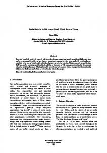
SIMULATIONS RESULTS Figures 2 and 3 compare the mean square range errors (MSREs) of the AOA based LS, WLS and CTLS algorithms as well as CRLB. The MSRE was defined as
Monte-Carlo simulations had been performed to evaluate the performance of the proposed AOA based CTLS location algorithm by compared with LS and WLS algorithms as well as Cramer-Rao lower bound (CRLB). For simplicity, we assumed that a ten-sensor geometry was employed with the sensors locating at [−42, −12], [−26, 30], [−8, 40], [16, 18], [36, 6], [24, −36], [−12, −24], [−20, 0], [15, −15], and [−30, −40] m in the presence of zero-mean and additive Gaussian noises in the AOA measurements. The source location was [xs, ys] = [0, 0] m. All results were averages of 10000 independent runs.
2 2 E xs xˆs ys yˆs , and its unit was m2. In Fig.
2, the minimum sensor number was 3, and the sensors were added successively. It is observed that the MSRE generally decreases as the sensor number increases in Fig. 2 and MSRE grows as the angle error variance increases in Fig. 3. Both Figs. 2 and 3 show that the proposed CTLS algorithm possesses the same performance as WLS and they both outperform LS. However, it is noticed that WLS requires a priori knowledge of the angle errors, which is usually not available or hard to be obtained in practical applications. Hence, CTLS algorithm is more suitable for practical location applications.
0.3
LS WLS CTLS CRLB
2
mean square range error (m )
0.25
V.
0.2
CONCLUSIONS
The AOA based CTLS location algorithm, which does not require a priori knowledge of the angle errors, has been proposed. Simulation results demonstrate that the performance of CTLS algorithm is close to the CRLB and CTLS algorithm is preferred compared with WLS algorithm in practical scenarios.
0.15
0.1
0.05
REFERENCES 0
3
4
5
6
7
8
9
[1]
10
number of sensors
[2]
Fig. 2 Mean square range error versus number of sensors under −40 dBrad2 angle error variance
[3] 0.1
LS WLS CTLS CRLB
0.08
2
mean square range error (m )
0.09
0.07
[4]
[5]
0.06 0.05 0.04
[6]
0.03 0.02 0.01 0 -50
-48
-46
-44
-42
-40
2
angle error variance (dBrad )
Fig. 3 Mean square range error for 6-sensor geometry
515
D.J. Torrieri, “Statistical theory of passive location systems,” IEEE Trans. Aerosp. Electron. Syst., vol. 20, no. 2, Mar. 1984, pp. 183-197. A. Pages-Zamora, J. Vidal, and D. H. Brooks, “Closed-form solution for positioning based on angle of arrival measurements,” Proc. PIMRC, Sep. 2002, pp. 1522–1526. K. W. Cheung, H. C. So, W. -K. Ma, and Y. T. Chan, “A constrained least squares approach to mobile positioning: Algorithms and optimality,” Eurasip J. Appl. Signal Process., vol. 2006, 2006, pp. 123. T. J. Abatzoglou, “Constrained total least squares applied to superresolution array processing,” Proc. MILCOM, 1990, pp. 11291132. T. J. Abatzoglou, J. M. Mendel, and G. A. Harada, “The constrained total least squares technique and its applications to harmonic superresolution,” IEEE Trans. Signal Process., vol. 39, no. 5, May 1991, pp. 1070-1087. K. Yang, J. An, X. Bu, and G. Sun, “Constrained Total Least-Squares Location Algorithm Using Time-Difference-of-Arrival Measurements,” IEEE Trans. Veh. Technol., vol. 59, no. 3, March 2010, pp. 1558-1562.