May 21, 2017 - ZEÃV RUDNICK AND EZRA WAXMAN. Abstract. Fermat showed that every ..... For these, the maximal gap is al- most surely of order log N/N, ...
ANGLES OF GAUSSIAN PRIMES
arXiv:1705.07498v1 [math.NT] 21 May 2017
´ RUDNICK AND EZRA WAXMAN ZEEV Abstract. Fermat showed that every prime p = 1 mod 4 is a sum of two squares: p = a2 + b2 . To any of the 8 possible representations (a, b) we associate an angle whose tangent is the ratio b/a. In 1919 Hecke showed that these angles are uniformly distributed as p varies, and in the 1950’s Kubilius proved uniform distribution in somewhat short arcs. We study fine scale statistics of these angles, in particular the variance of the number of such angles in a short arc. We present a conjecture for this variance, motivated both by a random matrix model, and by a function field analogue of this problem, for which we prove an asymptotic form for the corresponding variance.
Contents 1. Introduction 1.1. Angles of Gaussian primes 1.2. The number variance 1.3. A function field analogue 2. Repulsion between angles 2.1. Repulsion and its consequences 2.2. Deviations from randomness 2.3. The variance in the trivial regime 3. Almost all sectors contain an angle 3.1. A smooth count 3.2. Variance in the trivial regime 3.3. An upper bound 4. Relation to zeros of Hecke L-functions 4.1. Hecke characters and their L-functions 4.2. An Explicit Formula 4.3. Primes vs prime powers 4.4. Proof of Theorem 3.2 5. A random matrix theory model 5.1. The model 5.2. Proof of Proposition 5.3 6. A function field model 6.1. The group of sectors 6.2. Super-even characters and their L-functions Date: May 23, 2017. 1
2 2 3 5 7 7 8 8 10 10 11 12 13 13 14 17 20 20 21 23 24 24 26
´ RUDNICK AND EZRA WAXMAN ZEEV
2
6.3. A weighted count 6.4. The variance of Ψk,ν 6.5. Proof of Theorem 6.7 6.6. Relation between variance of Nk,ν and Ψk,ν 6.7. Proof of Lemma 6.11 References
27 29 31 31 33 34
1. Introduction 1.1. Angles of Gaussian primes. An odd prime p is a sum of two squares if and only if p = 1 mod 4, and in that case there are exactly 8 representations. Each representation corresponds to a Gaussian integer a + ib = √ iθa,b pe . We wish to understand the statistics of the resulting angles. It is useful to formulate the results in terms of prime ideals of the ring of Gaussian integers Z[i], which is the ring of integers of the imaginary quadratic field Q(i). The basic infra-structure that we need is complex conjugation z 7→ z¯, the norm map Norm : Q(i)× → Q× , Norm(z) = z z¯, and the norm one elements 1 SQ = {z ∈ Q(i) : Norm(z) = 1} = Q(i) ∩ S 1 .
For a Gaussian number α ∈ Q(i)× , we have a direction vector given by α u(α) := ( )2 ∈ S1Q α ¯ 4iθ so that u(α) = e , θ = arg α. Let p be a prime ideal in Z[i]. If p = hαi is generated by the Gaussian integer α, we associate a direction vector u(p) := u(α) ∈ S1Q . Since all generators of the ideal differ by multiplication by a unit Z[i]× = {±1, ±i}, the direction vector u(p) = ei4θp is well-defined on ideals, while the angle θp is only defined modulo π/2. We can choose θp to lie say in [0, π/2), corresponding to taking α = a + ib, with a > 0, b ≥ 0. Hecke [5] showed that as p varies over prime ideals of Z[i], the angles θp become uniformly distributed in [0, π2 ): For a fixed sector, defined by an interval I ⊆ [0, π2 ), (1.1)
#{Norm p ≤ x : θp ∈ I} |I| ∼ , #{Norm p ≤ x} π/2
x→∞
where |I| is the length of the interval I. The validity of (1.1) for shrinking sectors was studied by Kubilius and his school [11, 12, 10, 14, 15, 16], obtaining that (1.1) holds for any sector as long as |I| > x−δ for some 1/4 < δ < 1/2. See also [4] for existence of prime angles in somewhat smaller sectors without the full force of (1.1). Assuming the Generalized Riemann Hypothesis (GRH), we know that (1.1) holds for intervals with length(I) � x−1/2+o(1) . This regime is the limit of what can be expected to hold for individual sectors, because it is easy
ANGLES OF GAUSSIAN PRIMES
3
to see that there are no Gaussian integers (let alone primes) in the sector {a, b > 0 : a2 + b2 ≤ x, 0 < arctan ab < x−1/2 }. Hence for smaller sectors we can only hope for a statistical theory, rather than individual results. To formulate the theory, we introduce some notation: Given x � 1, let N be the number of prime ideals p ⊂ Z[i] of norm at most x x N := #{p prime : Norm p ≤ x} ∼ log x π by the Prime Ideal Theorem for Q(i). Given an interval IK (θ) = [θ − 4K , θ+ π ] of length π/(2K) centered at θ, define a sector 4K
Sect(θ, x) = {z ∈ C : Norm(z) = z z¯ ≤ x, arg(z) ∈ IK (θ)} √ of radius x and opening angle defined by IK (θ). Given K � 1, we divide the interval [0, π/2) into K disjoint arcs IK (θ1 ), . . . , IK (θK ) of equal length, which in turn define K disjoint sectors Sect(θj , x), and study the number of prime angles falling into each such sector. If the sectors are too small, in the sense that the number K of sectors is larger than the number N of angles involved, then the typical such sector will not contain any Gaussian prime. We want to show that in the range K � N 1−� , almost all sectors with opening angles of size ≈ 1/K contain at least one angle θp , Norm(p) ≤ x. We can do so assuming GRH (for the family of Hecke L-functions): Theorem 1.1. Assume GRH. Then almost all arcs of length 1/K contain at least one angle θp for a prime ideal with Norm(p) ≤ K(log K)2+o(1) . Unconditionally, one may use zero-density theorems as in [16] to obtain a result with Norm(p) < K 2−δ for some small δ > 0. It is surprising that something like Theorem 1.1 does not seem to have been considered long ago. It has come up independently in the recent work of Ori Parzanchevski and Peter Sarnak [17]. 1.2. The number variance. One way to obtain such an “almost-everywhere” result is by computing the variance of a suitable counting function. The study of the structure of the variance is the main point of this paper. Let (1.2)
NK,x (θ) = #{p prime, Norm p ≤ x, θp ∈ IK (θ)}
be the number of angles θp in IK (θ). The expected number is Z π/2 N dθ = . hNK,x i := NK,x (θ) π/2 K 0 We wish to study the number variance Z π/2 2 dθ Var(NK,x ) = N − hN i . K,x K,x π/2 0
´ RUDNICK AND EZRA WAXMAN ZEEV
4
If N = o(K), then for almost all intervals, we do not have any angles θp in the interval IK (θ). We can easily compute the variance in this “trivial” regime: N Var(NK,x ) ∼ , N = o(K) . K For the interesting range, when K � N 1−� , we expect: Conjecture 1.2. For 1 � K � N 1−o(1) log K N min(1, 2 ). Var(NK,x ) ∼ K log N For random angles (N uniform independent points in [0, π/2)), the variance would be ∼ N/K. Thus we expect the Gaussian angles to display a marked deviation from randomness, in that there is a crossover from purely random behaviour for very short intervals (K � N 1/2 ), to a saturation for moderately short intervals (1 � K � N 1/2 ), where the variance is smaller than that of random angles; so they display some measure of rigidity. See Figure 1 for numerical evidence. For an explanation of the underlying rigidity present here and for other deviations from randomness, see § 2. A related saturation effect was previously observed by Bui, Keating and Smith [2], in the context of computing the variance of sums in short intervals of coefficients of a fixed L-function of higher degree. 1.0
0.8
0.6
0.4
0.2
0.2
0.4
0.6
0.8
1.0
Figure 1. A plot of the ratio Var(NK,x )/E(NK,x ) versus β = log K/ log N , for X ≈ 108 . The smooth line is min(1, 2β). One of our main goals is to justify Conjecture 1.2. In § 3 we define a suitably smoothed version of the counting function NK,x and express the corresponding variance in terms of zeros of a family of Hecke L-functions. This enables us, in § 4, to use GRH to give an upper bound for this variance and consequently deduce the almost-everywhere result of Theorem 1.1. Moreover, in § 5 we go on to develop a suitable random-matrix theory model of this result, which gives a result corresponding to Conjecture 1.2. We now
ANGLES OF GAUSSIAN PRIMES
5
turn to formulating a similar problem in a function field setting, where we can prove an analogue of Conjecture 1.2. 1.3. A function field analogue. Let Fq be a finite field of cardinality q, from now on assumed to be odd. We want to write prime (irreducible monic) polynomials as P (T ) = A(−T )2 + T B(−T )2
(1.3)
which for monic primes P (T ) is equivalent to the constant term P (0) being a square in Fq (see e.g. [1]). If additionally P (0) 6= 0, then there are exactly four such representations, obtained from (1.3) by changing √ the signs√of A and B. This decomposition gives a factorization in Fq [T ][ −T ] = Fq [ −T ] as √ √ ˜ = (A + −T B)(A − −T B) P =p·p and the corresponding factorization of the ideal (P ) ⊂ Fq [T ] into a pair of √ −T ]. The number N of such prime polynoconjugate prime ideals of F [ q √ mials p( −T ) of degree ν with p(0) 6= 0 satisfies q ν/2 qν + O( ) ν ν √ by the Prime Polynomial Theorem in F [ −T ]. q √ √ Denote by S = −T and consider the quadratic extension Fq (T )( −T ) = Fq (S), which is still rational (genus zero). Let Fq [[S]] be the ring of formal power series. It is equipped with the Galois involution N=
σ : S 7→ −S,
σ(f )(S) = f (−S) ,
and the norm map Norm : Fq [[S]]× → Fq [[T ]]× ,
Norm(f ) = f (S)f (−S) .
We denote S1 := {g ∈ Fq [[S]]× : g(0) = 1, Norm(g) = 1} the formal power series with constant term 1 and unit norm. This is a group, which is our analogue of the unit circle. It is important to note that since q is odd, Hensel’s Lemma tells us that the square map u 7→ u2 is an 1 1 automorphism √ of S , and in particular each element of S admits a unique square root u. We put an absolute value |f | = q − ord(f ) on Fq [[S]], where ord(f ) = max(j : S j | f ). We then divide S1 into “sectors” Sect(u; k) = {v ∈ S1 : |v − u| ≤ q −k } . We denote by S1k = {f ∈ Fq [S]/(S k ) : f (0) = 1, Norm(f ) := f (−S)f (S) = 1 mod S k }
´ RUDNICK AND EZRA WAXMAN ZEEV
6
� �× the elements of unit norm and constant term unity in Fq [S]/(S k ) . The group S1k parameterizes the different sectors. The order of S1k is K := #S1k = q κ , where k κ := b c, 2
( 2κ + 1 so that k = 2κ
.
We next want to define the notion of√direction (essentially √ an angle) for any nonzero polynomial f = A(−T ) + −T B(−T ) ∈ Fq [ −T ]. To motive the definition below, recall that for a nonzero complex number α = |α|eiθ , we have α/α = e2iθ . To any nonzero f ∈ Fq [S] which is coprime to S, we associate a norm-one element U (f ) ∈ S1 via the map s f . (1.4) U : f 7→ σ(f ) Note that since f (0) 6= 0, f /σ(f ) has constant term p one, lies 1in Fq [[S]], and 1 has unit norm, that is f /σ(f ) ∈ S , and hence f /σ(f ) ∈ S exists and is unique. Moreover, U (cf ) = U (f ) for all scalars c ∈ F× q , so that if f ∈ Fq [S] then U (f ) only depends on the ideal (f ) ⊂ Fq [S] generated by f . We want to count the number of primes ideals (p) ⊂ Fq [S] with p(0) 6= 0, whose directions U (p) lie in a given sector. For u ∈ S1 , let Nk,ν (u) := # {(p) prime, p(0) 6= 0 : deg p = ν, U (p) ∈ Sect(u, k)} . The mean value is clearly hNk,ν i :=
N q ν /ν 1 X N (u) = ∼ . k,ν qκ K qκ 1 u∈Sk
For k ≤ ν we can show that as q → ∞, N + O(νq ν/2 ) (1.5) Nk,ν (u) = K which gives an asymptotic result if κ < ν/2. For larger values of κ, there are sectors which do not contain prime directions, as in the number field case, see Remark 6.6. Our main result is the computation, in the large q limit, of the number variance 2 1 X Var(Nk,ν ) := κ Nk,ν − hNk,ν i . q 1 u∈Sk
Theorem 1.3. Assume that κ ≥ 3, or if κ = 2 that 5 - q. Then as q → ∞, ( 2κ − 2, ν ≥ 2κ − 2 q ν−κ Var(Nk,ν ) ∼ 2 × ν ν − 1 + η(ν), κ ≤ ν ≤ 2κ − 2 where η(ν) = 1 if ν is even, and 0 otherwise.
ANGLES OF GAUSSIAN PRIMES
7
To compare it to our number field conjecture, here the number of sectors is K = q κ , the number of directions (i.e. of Gaussian prime ideals p of degree ν) is N ∼ q ν /ν, so that the expected value is N/K, and the variance satisfies, as q → ∞, log K q 2 1 2 logq N − logq N , logq K ≤ 2 logq N + 1 Var(Nκ,ν ) ∼ N/K 1 1 + η(logq N )−1 , log N 2 logq N + 1 ≤ logq K ≤ logq N . q
Our conjecture 1.2 for the number-field variance is Var(NK,N ) log K ∼ min(1, 2 ) N/K log N which is analogous to the above. Acknowledgments We thank Steve Lester, for his help in the beginning of the project, and Jon Keating and Peter Sarnak for their comments. The research leading to these results has received funding from the European Research Council under the European Union’s Seventh Framework Programme (FP7/2007-2013) / ERC grant agreement no 320755. 2. Repulsion between angles 2.1. Repulsion and its consequences. Let a be a nonzero ideal in Z[i]. If a = hαi is generated by the Gaussian integer α, we associate a direction vector u(p) := u(α) ∈ S1Q . Since all generators of the ideal differ by multiplication by a unit Z[i]× = {±1, ±i}, the direction vector u(a) = ei4θa is well-defined on ideals, while the angle θa is only defined modulo π/2. We can choose θa to lie say in [0, π/2), corresponding to taking α = a + ib, with a > 0, b ≥ 0. If a = hαi for non-zero α ∈ Z, then θa = 0. Lemma 2.1. i) If θa 6= 0 then 1 θa � √ Norm a ii) If p 6= q are ideals with distinct angles θp 6= θq then |θp − θq | ≥ √
1 Norm p Norm q
Proof. i) Write a = ha + ibi with a, b > 0. Then b 1 1 1 ≥ ≥√ =√ . 2 2 a a a +b Norm a √ Since we may assume that θa ∈ (0, π/4), we have tan θa ≤ 2θa which gives our claim. ii) Write p = ha + ibi, q = hc + idi, with a, b > 0 and c > 0, d ≥ 0. Consider the triangle having vertices at the origin, a + ib and c + id. Since tan θa =
8
´ RUDNICK AND EZRA WAXMAN ZEEV
θp 6= θq , its area is positive and being a lattice triangle, its area is at least 1/2. On the other hand, its area is given in terms of the angle θp − θq between the sides a + ib and c + id as p 1p area = Norm p Norm q sin |θp − θq | . 2 Thus we find p p Norm p Norm q| sin(θp − θq )| ≥ 1 and hence |θp − θq | ≥ sin |θp − θq | ≥ √
1 . Norm p Norm q �
√ Lemma 2.1 implies that the interval {0 < θ < 1/ x} will contain no angles θp for Norm p � x, so that the number NK,x of prime angles θp in this interval is zero. Hence we cannot expect an asymptotic formula NK,x ∼ N/K to hold for all intervals if K � N 1/2 , while it does hold (assuming GRH) for larger intervals. Theorem 1.1 guarantees that almost all intervals will contain angles if K � N 1−o(1) . 2.2. Deviations from randomness. The existence of a “big hole” as above displays a striking deviation from randomness of the angles, when compared to N random angles in [0, π/2). For these, the maximal gap is almost surely of order log N/N , while Lemma 2.1(i) guarantees a much larger gap, of size N −1/2−o(1) . Another statistic which indicates that Gaussian angles behave differently than random points is the minimal spacing statistic: For N random angles in [0, π/2) as above, the smallest gap is almost surely of size ≈ 1/N 2 [13]. In contrast, the minimal gap between the angles {θp 6= 0 : Norm p ≤ x} is by Lemma 2.1 1 1 min{|θp − θp0 | : Norm p, Norm p0 ≤ x, p 6= p0 } � ≈ x N log N which is much bigger than the random case. 2.3. The variance in the trivial regime. We want to study fluctuations in the number NK,x of angles falling in “random” short intervals. Take the interval length 1/K = o(1/x), equivalently the number K of intervals, is much larger than the number N ∼ x/ log x of angles: N = o(K). Then for almost all intervals, we do not have any angles θp in the interval IK (θ). Nonetheless we can compute the variance in this “trivial” regime. Proposition 2.2. If x = o(K) then Var(NK,x ) ∼
N K
ANGLES OF GAUSSIAN PRIMES
9
π Proof. We recall the definition (1.2): Given an interval IK (θ) = [θ − 4K ,θ+ π 1 4K ] of length π/2K centered at θ, let X NK,x (θ) = #{p prime, Norm p ≤ x : θp ∈ IK (θ)} = IK (θp − θ) Norm p≤x prime
be the number of prime angles θp in IK (θ). We will take the center θ of the interval to be random, i.e. uniform in (0, π/2). We compute the second moment of N = NK,x using its definition X X
2� N = hIK (θp − θ)IK (θq − θ)i Norm p≤x Norm q≤x
where throughout we use 1 hHi := π/2
Z
π/2
H(θ)dθ . 0
The contribution of pairs of inert primes, where θp = 0, p = hpi, p = 3 mod 4, Norm p = p2 ≤ x, is � � √ �2
#{p = 3 mod 4, p ≤ x} · IK (−θ)2 . 2 = I and Note that IK K
� length(IK ) 1 IK (−θ)2 = hIK (θ)i = = . π/2 K √ √ Moreover, the number of p = 3 mod 4, p�≤ x is �� x/ log x. Hence the x contribution of pairs of inert primes is O K(log . x)2 If p 6= q and at least one of p, q is not inert, so that θp 6= θq , then Lemma 2.1 gives 1 |θp − θq | ≥ . x For the integral hIK (θp − θ)IK (θq − θ)i to be nonzero, it is necessary that there be some θ so that both θp , θq ∈ IK (θ), which forces the distance between the two angles to be at most π/2K: π . |θp − θq | ≤ 2K Hence if x = o(K) then such off-diagonal pairs contribute nothing. We conclude that the second moments of NK,x is essentially given by the sum of the diagonal terms � � X
2� � x N = IK (θp − θ)2 + O K(log x)2 Norm p≤x � � N X 1 x = +O ∼ . K K(log x)2 K Norm p≤x
1We abuse notation and use the same symbol for the interval and its indicator function.
10
´ RUDNICK AND EZRA WAXMAN ZEEV
We can now compute the variance:
� N N Var(N ) = N 2 − hN i2 ∼ − ( )2 . K K Since N = o(K) we find N Var(N ) ∼ K as claimed.
�
3. Almost all sectors contain an angle 3.1. A smooth count. Our goal in this section is to prove Theorem 1.1, which claims (assuming GRH) that in the non-trivial range K � X 1−� , almost all arcs of size ≈ 1/K contain at least one angle θp , Norm(p) ≤ X. We can do so assuming GRH (for the family of Hecke L-functions). To count the number of angles θp lying in a short segment of [0, π/2), pick a window function f ∈ Cc∞ (R), which we take to be even and real valued, and for K � 1 define X π K (θ − j )) FK (θ) := f( π/2 2 j∈Z
which is π/2-periodic, and localized on a scale of 1/K. The Fourier expansion of FK is X k 1 (3.1) FK (θ) = FbK (k)ei4kθ , FbK (k) = fb( ) K K k∈Z R∞ where the Fourier transform is normalized as fb(y) = −∞ f (x)e−2πiyx dx. Note that since f is even and real valued, the same holds for fb. Let Φ ∈ Cc∞ (0, ∞). Now set X Norm p prime (θ) := Φ( ψK,X ) log Norm(p)FK (θp − θ) X p prime
the sum over all prime ideals of Z[i], which gives a smooth count of prime angles θp lying in a smooth window defined FK around θ. We also define X Norm a ψK,X (θ) := Φ( )Λ(a)FK (θa − θ) X a the sum over all powers of prime ideals, with the von Mangoldt function Λ(a) = log Norm(p) if a = pr is a power of a prime ideal p, and equal to zero otherwise. We next compute the mean value. prime Lemma 3.1. The mean values of ψK,X and ψK,X are asymptotically Z ∞ D E XZ ∞ prime (3.2) hψK,X i ∼ ψK,X ∼ f (x)dx Φ(u)du . K −∞ 0
ANGLES OF GAUSSIAN PRIMES
11
Moreover, D E X 1/2 prime . hψK,X i − ψK,X � K Proof. The mean value is hψK,X i =
X Norm p 1 b f (0) Φ( )Λ(p) . K X p prime
We can evaluate this using the Prime Ideal Theorem to obtain: Z Z ∞ X ∞ f (x)dx Φ(u)du , hψK,X i ∼ K −∞ 0 D E prime . If in addition we use GRH, we obtain a remainder and likewise for ψK,X 1/2
term of O( XK ) for both. We bound the difference by E D prime = hψK,X i − ψK,X
X
Λ(a)Φ(
a6=prime
�
1 K
X
Norm a fb(0) ) X K
Λ(a) �
Norm(a)�X a6=prime
X 1/2 K
which shows that the mean values are close.
�
Note that the inert primes p = hpi give angle θp = 0, but that Norm p = √ prime , we get a contribution of size X if θ ≈ 0. This is so that in ψK,X significantly larger than the mean value if K � X 1/2 .
p2
prime 3.2. Variance in the trivial regime. The variance of ψK,X in the trivial regime X = o(K) is:
(3.3)
prime Var(ψK,X ) ∼ Var(ψK,X ) ∼ c2 (f, Φ) ·
X log X , K
where Z
∞
c2 (f, Φ) :=
2
Z
f (y) dy −∞
∞
Φ(t)2 dt .
0
Indeed, if X = o(K) then the same argument of repulsion between angles as in § 2.3 allows us to compute the second moment as asymptotically equal to the sum over the diagonal pairs
�
� X Norm(a) 2 |ψK,X |2 ∼ |FK (θ)|2 Φ( ) Λ(a)2 . X a
´ RUDNICK AND EZRA WAXMAN ZEEV
12
By Parseval’s theorem, we have Z π/2 X
� 1 2 |FK (θ)| = |FK (θ)|2 dθ = |FbK (k)|2 π/2 0 k∈Z Z 1 ∞ 1 Xb k 2 = 2 f( ) ∼ f (y)2 dy K K K −∞ k∈Z
and X a
Norm(a) 2 Φ( ) Λ(a)2 ∼ X
Z
∞
Φ(t)2 dt · X log X
0
by the Prime Ideal Theorem. This gives the second moment as Z ∞ E Z ∞ D X log X prime 2 2 f (y) dy Φ(t)2 dt · |ψK,X | ∼ , K −∞ 0 and since X = o(K), we obtain (3.3) for Var(ψK,X ). The argument for prime ) is identical. Var(ψK,X 3.3. An upper bound. We will give an upper bound on the variance of prime ψK,X in the non-trivial regime K � X, assuming GRH: Theorem 3.2. Assume GRH. Then prime Var(ψK,X )�
X (log K)2 . K
From this bound we easily deduce Theorem 1.1: Proof. We use Chebyshev’s inequality and Theorem 3.2 to deduce: � � prime ) Var(ψK,X 1 prime prime prime Prob θ : |ψK,X (θ) − E(ψK,X )| > E(ψK,X ) ≤ 1 prime 2 2 4 (EψK,X )) �
X 2 K (log K) X 2 (K )
�
K(log K)2 . X
Taking X = K(log K)2+o(1) we find that for almost all θ, prime ψK,X (θ) �
X K
prime is nonzero. Therefore the sum defining ψK,X is non-empty, and since it is a sum over prime ideals giving angles θp in the arc of length ≈ 1/K around θ, we find that for almost all θ, such arcs contain an angle θp for a prime ideal with Norm(p) ≤ X = K(log K)2+o(1) . �
ANGLES OF GAUSSIAN PRIMES
13
4. Relation to zeros of Hecke L-functions 4.1. Hecke characters and their L-functions. The Hecke characters Ξk (α) = (α/¯ α)2k , k ∈ Z, give well defined functions on the ideals of Z[i]. In terms of the angles associated to ideals, we have ei4kθp = Ξk (p). To each such character Hecke [5] associated its L-function L(s, Ξk ) =
X 06=a⊆Z[i]
Y Ξk (a) (1 − Ξk (p)(Norm p)−s )−1 , = s (Norm a) p
Re(s) > 1 .
prime
Note that L(s, Ξk ) = L(s, Ξ−k ). Hecke showed that if k 6= 0, these functions have an analytic continuation to the entire complex plane, and satisfy a functional equation: (4.1)
ξk (s) := π −(s+2|k|) Γ(s + 2|k|)L(s, Ξk ) = ξk (1 − s) .
The completed L-function ξk (s) has all its zeros in the critical strip 0 < Re(s) < 1 (the non-trivial zeros of L(s, Ξk )), and the Generalized Riemann Hypothesis asserts that they all lie on the critical line Re(s) = 1/2. The growth of the number of nontrivial zeros of L(s, Ξk ) in a fixed rectangle is (4.2)
#{ρ : 0 ≤ Im(ρ) ≤ T0 } ∼
T0 log k , π
in other words, the density of zeros is
k → ∞,
T0 > 0 fixed,
log |k| π .
Lemma 4.1. (4.3)
ψK,X (θ) =
X
e−i4kθ
k
1 b k X Norm a f( ) Φ( )Λ(a)Ξk (a) K K a X
and (4.4)
prime ψK,X (θ) =
X
e−i4kθ
1 b k X Norm p f( ) Φ( )Λ(p)Ξk (p) . K K X p prime
k
Proof. Inserting the Fourier expansion (3.1) of FK gives prime ψK,X (θ) =
X k
e−i4kθ
1 b k X Norm p f( ) Φ( )Λ(p)ei4kθp . K K p X
Now note that ei4kθp = Ξk (p) is the Hecke character, to obtain (4.4). The same argument gives (4.3). � The zero mode k = 0 in (4.4) is the mean value (3.2). The same holds for ψK,X .
14
´ RUDNICK AND EZRA WAXMAN ZEEV
4.2. An Explicit Formula. Proposition 4.2. Let Φ ∈ Cc∞ (0, ∞), and Z ∞ dx ˜ Φ(x)xs Φ(s) = x 0 be its Mellin transform. Then for k 6= 0 and X �Φ 1, X X Norm(a) ρ ˜ Λ(a)Ξk (a)Φ( Φ(ρ)X )=− X a ξk (ρ)=0 � Z � 0 1 Γ Γ0 s ˜ + (s + 2|k|) + (1 − s + 2|k|) Φ(s)X ds 2πi (2) Γ Γ where the sum on the RHS is over all non-trivial zeros of L(s, Ξk ). Proof. Lk (s) := L(s, Ξk ). Using Mellin inversion Φ(x) = R We abbreviate 1 −s ds we obtain ˜ Φ(s)x 2πi Re(s)=2 Z X X Xs Norm(a) 1 ˜ Λ(a)Ξk (a) Λ(a)Ξk (a)Φ( )= Φ(s)ds s X 2πi Norm(a) (2) a a Z L0 1 s ˜ = − k (s)Φ(s)X ds . 2πi (2) Lk In terms of the completed L-function ξk (s), the logarithmic derivative of L(s, Ξk ) is L0 ξ0 Γ0 − k (s) = − log π + (s + 2|k|) − k (s) . Lk Γ ξk Inserting into the above gives Z Z � � L0k 1 Γ0 1 s s ˜ ˜ − (s)Φ(s)X ds = − log π + (s + 2|k|) Φ(s)X ds 2πi (2) Lk 2πi (2) Γ Z ξ0 1 s ˜ − k (s)Φ(s)X ds . + 2πi (2) ξk We shift the contour in the integral to Re(s) = −1, picking up the poles ξ0 of − ξkk (s), which are all simple poles with residue −1 at the non-trivial zeros of Lk (s), giving Z Z X ξk0 ξ0 1 1 s ρ s ˜ ˜ ˜ Φ(ρ)X + ds . − (s)Φ(s)X ds = − − k (s)Φ(s)X 2πi (2) ξk 2πi ξ k (−1) ρ Changing variables s 7→ 1 − s gives Z Z ξk0 ξ0 1 1 s ˜ ˜ − s)X 1−s ds . − (s)Φ(s)X ds = − k (1 − s)Φ(1 2πi (−1) ξk 2πi (2) ξk The functional equation (4.1) of L(s, Ξk ) implies −
ξk0 ξ0 (s) = k (1 − s) ξk ξk
ANGLES OF GAUSSIAN PRIMES
15
which gives Z Z ξk0 ξk0 1 1 1−s ˜ ˜ − s)X 1−s ds . − (1 − s)Φ(1 − s)X ds = (s)Φ(1 2πi (2) ξk 2πi (2) ξk Returning to the incomplete L-function gives Z ξk0 1 ˜ − s)X 1−s ds (s)Φ(1 2πi (2) ξk � Z � L0k 1 Γ0 ˜ − s)X 1−s ds = − log π + (s + 2|k|) + (s) Φ(1 2πi (2) Γ Lk Z Z Γ0 1 1 s s ˜ ˜ Φ(s)X ds + (1 − s + 2|k|)Φ(s)X ds = − log π 2πi (2) 2πi (2) Γ Z L0k 1 ˜ − s)X 1−s ds . + (s)Φ(1 2πi (2) Lk By Mellin inversion, 1 2πi
Z
1 s ˜ Φ(s)X ds = Φ( ) X (2)
which vanishes for X � 1 as Φ is compactly supported in (0, ∞). Likewise, 1 2πi
Z (2)
Z X L0k 1 Λ(a)Ξk (a) 1−s ˜ 1−s ˜ (s)Φ(1 − s)X ds = − X Φ(1 − s)ds Lk 2πi (2) a Norm(a)s X Λ(a)Ξk (a) 1 Z ˜ − s)(X Norm(a))1−s ds =− Φ(1 Norm(a) 2πi (2) a X Λ(a)Ξk (a) 1 =− Φ( )=0 Norm(a) X Norm(a) a
since each term vanishes for X � 1 (independently of a, since Norm(a) ≥ 1). Collecting terms, we find X
X Norm(a) ρ ˜ )=− Φ(ρ)X X ρ � Z � 0 1 Γ Γ0 s ˜ + (s + 2|k|) + (1 − s + 2|k|) Φ(s)X ds 2πi (2) Γ Γ
Λ(a)Ξk (a)Φ(
a
as claimed. Lemma 4.3. For k 6= 0, � Z � 0 1 Γ Γ0 X 1/2 log 2|k| s ˜ (s + 2|k|) + (1 − s + 2|k|) Φ(s)X ds � . 2πi (2) Γ Γ (log X)100
�
´ RUDNICK AND EZRA WAXMAN ZEEV
16
Proof. Note that the integrand is analytic in −2 < Re(s) < 3, so we may shift the contour of integration to Re(s) = 1/2. Let � 0 � Γ 1 Γ0 1 ˜ 1 + it) . hk (t) := ( + it + 2|k|) + ( − it + 2|k|) Φ( Γ 2 Γ 2 2 The integral is essentially X 1/2 times the Fourier transform b hk (log X), that is Z ∞ 1/2 1 X hk (t)eit log X dt . 2π −∞ We can estimate the derivatives of hk (t) by using Stirling’s formula and the ˜ 1 + it) as being bounded by rapid decay of Φ( 2 (j)
|hk (t)| �
log 2|k| . (1 + |t|)200
Hence integration by parts shows that the Fourier transform of hk is bounded by log 2|k| |b hk (log X)| � (log X)100 which proves the Lemma. � From Lemma 4.1, Proposition 4.2 and Lemma 4.3 we deduce: Corollary 4.4. Assume GRH. Then ψK,X (θ) − hψK,X i = −X 1/2
X
e−i4kθ
k6=0
1 b k f( ) K K
log K ˜ 1 + iγk,n )X iγk,n + O Φ( . 100 2 (log X) �
X
ξk ( 12 +iγk,n )=0
�
Averaging Corollary 4.4 over θ we find Corollary 4.5. Assume GRH. Then Var(ψK,X ) = 2
X X b k 2 f( ) K2 K k6=0
X ξk ( 12 +iγk,n )=0
log K ˜ 1 + iγk,n )X iγk,n + O Φ( . 2 (log X)100 �
Corollary 4.6. Assume GRH. Then Var(ψK,X ) �
X (log K)2 , K
Proof. We use GRH to obtain |X iγk,n | = 1 so that X 1 X iγ k,n ˜ ˜ 1 + iγk,n )| . (4.5) Φ( + iγk,n )X |Φ( ≤ n 2 2 n
�
ANGLES OF GAUSSIAN PRIMES
17
We use a standard bound for the number of zeros of L(s, Ξk ) in an interval (see [6, Proposition 5.7]): 1 #{n : Im(ρn,k ) ∈ [T − 1, T + 1]} � log(| + iT | + 2|k|) . 2
(4.6)
˜ decays rapidly in vertical strips, say: Note that Φ 1 ˜ 1 + iu)| �Φ |Φ( 2 (1 + |u|)100 which together with (4.6) gives | (4.7)
X n
˜ 1 + iγk,n )| ≤ Φ( 2
X
X
j∈Z n:j≤γk,n 0
as claimed.
�
4.3. Primes vs prime powers. We pass from a sum over prime ideals to a sum over all prime powers: Lemma 4.7. Assume GRH. For k 6= 0 such that log |k| � log X, X
Λ(a)Ξk (a)Φ(
a
� � X Norm(a) Norm(p) )= Λ(p)Ξk (p)Φ( ) + O X 1/3 . X X p prime
Proof. We denote Σprime (X, k, Φ) :=
X
Λ(p)Ξk (p)Φ(
p prime
Norm(p) ) X
and Σall (X, k, Φ) :=
X a
Λ(a)Ξk (a)Φ(
Norm(a) ). X
Assuming GRH, we have Σall (X, k, Φ) � X 1/2 log(2|k|) .
´ RUDNICK AND EZRA WAXMAN ZEEV
18
Indeed, from the Explicit Formula (Proposition 4.2), Lemma 4.3 and GRH we have X ˜ 1 + iγ)X 21 +iγ Σall (X, k, Φ) = − Φ( 2 ξk ( 21 +iγ)=0 � Z � 0 1 Γ Γ0 s ˜ + (s + 2k) + (1 − s + 2k) Φ(s)X ds 2πi (2) Γ Γ 1/2 X ˜ 1 + iγ)| + X log 2|k| � X 1/2 log(2|k|) |Φ( � X 1/2 2 (log X)100 1 ξk ( 2 +iγ)=0
on using the density of zeros of L(s, Ξk ) (4.2). Next we crudely bound the contribution Σ≥2 (X, k, Φ) to Σall (X, k, Φ) of the higher prime powers pj , j ≥ 2: X X Norm(pj ) ) Σ≥2 (X, k, Φ) := Λ(pj )Ξk (pj )Φ( X p prime j≥2
X
≤
log Norm(p)
j≥2
p prime
X
�
X
Φ(
Norm(p)j ) X
log Norm(p)
p prime Norm(p)�X 1/2
log X log Norm(p)
� X 1/2 . Therefore we obtain a crude a priori bound on the contribution of primes: (4.8)
Σprime (X, k, Φ) = Σall (X, k, Φ) − Σ≥2 (X, k, Φ) � X 1/2 log(2|k|) .
We now seek a more refined estimate. In the sum Σall (X, k, Φ) over all prime power, we separately treat the contributions of primes, of squares of primes, and of higher powers: Σall (X, k, Φ) = Σprime (X, k, Φ) + Σ2 (X, k, Φ) + Σ≥3 (X, k, Φ) where Σ≥3 (X, k, Φ) :=
X X
Λ(pj )Ξk (pj )Φ(
p prime j≥3
Norm(pj ) ) X
and Σ2 (X, k, Φ) =
X p prime
=
X p prime
Λ(p2 )Ξk (p2 )Φ(
Norm(p2 ) ) X
log Norm(p)Ξ2k (p)Φ(
Norm(p)2 ). X
By definition, Σ2 (X, k, Φ) = Σprime (X 1/2 , 2k, Φ2 )
ANGLES OF GAUSSIAN PRIMES
19
where Φ2 (u) = Φ(u2 ). Therefore inputting the a priori bound (4.8) (which uses GRH to get cancellation) gives Σ2 (X, k, Φ) � X 1/4 log(2|k|) . For the contribution of higher powers, we use X X Norm(p)j Φ( Σ≥3 (X, k, Φ) � log Norm(p) ) X j≥3
p prime
X
�
log Norm(p)
p prime Norm(p)�X 1/3
log X log Norm(p)
� X 1/3 . Thus we obtain Σall (X, k, Φ) = Σprime (X, k, Φ) + O(X 1/4 log(2|k|)) + O(X 1/3 ) . Assuming that log |k| � log X gives us the result.
�
Lemma 4.8. Assume GRH. E D X 2/3 prime 2 | � |ψK,X − ψK,X K Proof. We use Lemma 4.1 to write X 1 X −i4kθ b k Norm a prime ψK,X (θ) − ψK,X (θ) = e f( ) Λ(a)Φ( )Ξk (a) . K K X k
a6=prime
The term k = 0 is the difference between mean values, which by Lemma 3.1 is O(X 1/2 /K). Hence prime ψK,X (θ) − ψK,X (θ) =
X 1 X −i4kθ b k Norm a X 1/2 f( ) e Λ(a)Φ( )Ξk (a) + O( ) K K X K k6=0
a6=prime
X 1/2 ) K
� say. Hence it suffices to show that I 2 � X 2/3 /K. We have 2
2� Norm a 1 X b k 2 X f( ) Λ(a)Φ( )Ξk (a) . I = 2 K K X = I + O(
k6=0
a6=prime
By Lemma 4.7, the sum over a non prime is O(X 1/3 ) (assuming log K � log X), and therefore
2� 1 X b k 2 2/3 X 2/3 I � 2 f( ) X � K K K k6=0
as desired.
�
´ RUDNICK AND EZRA WAXMAN ZEEV
20
4.4. Proof of Theorem 3.2. We want to show that D E X prime prime prime Var(ψK,X ) = ||ψK,X − ψK,X ||22 � (log K)2 K where Z π/2 1 2 ||f ||2 = |f (θ)|2 dθ π/2 0 is the standard L2 norm on [0, π/2]. Using the triangle inequality, we have D E prime prime prime ||ψK,X − ψK,X ||2 ≤ ||ψK,X − ψK,X ||2 + ||ψK,X − hψK,X i ||2 D E prime + | hψK,X i − ψK,X |. By Lemma 4.8 E1/2 � X 2/3 �1/2 D prime 2 prime | � − ψK,X ||2 = |ψK,X − ψK,X ||ψK,X ; K by Corollary 4.6, �1/2 � �1/2 �X , ||ψK,X − hψK,X i ||2 = Var(ψK,X ) � (log K)2 K and by Lemma 3.1, the mean values are close: E D X 1/2 prime . hψK,X i − ψK,X � K Thus we obtain E � X 2/3 �1/2 � X D �1/2 X 1/2 prime prime ||2 � − ψK,X ||ψK,X (log K)2 + + K K K �1/2 �X � (log K)2 K hence X prime Var(ψK,X ) � (log K)2 K which proves Theorem 3.2.
�
5. A random matrix theory model In this section we present a conjecture for the variance of the smooth count ψK,X : Conjecture 5.1. Var(ψK,X ) ∼ c2 (f, Φ) where Z
X · min(log X, 2 log K) K
∞
c2 (f, Φ) = −∞
f (y)2 dy
Z 0
∞
Φ(t)2 dt .
ANGLES OF GAUSSIAN PRIMES
21
Note that Conjecture 5.1 coincides with our result (3.3) in the trivial regime range K � X. To recover Conjecture 1.2 from Conjecture 5.1, we can (at a heuristic level) pass to an actual count with sharp cutoffs: Taking f = 1[−1/2,1/2] and Φ = 1(0,1] , and replace the weight Λ(p) by log X throughout, and ignore the contribution of higher powers of primes. We use Corollary 4.5 with X = K α for α > 0, and note that since fb is even, and ξ−k (s) = ξk (s), we can pass to a sum over positive k’s, to obtain 2 2X X b k 2 X ˜ 1 Φ( + iγk,j )eiα log Kγk,j , f( ) (5.1) Var(ψK,X ) ∼ 2 K K 2 j
k>0
the inner sums over all non-trivial zeros of L(s, Ξk ); we have ignored the remainder term in Corollary 4.5 as it can be seen to be o(X/K) by using (4.7). Let (5.2)
n :=
α log K , 2 π
and Sn (Ξk ) =
X j
˜ 1 + iγk,j )e2πinγk,j . Φ( 2
Since the density of zeros of L(s, Ξk ) is about ≈ log |k|, the sum in Sn (Ξk ) is over O(log K) zeros. Conjecture 5.1 is clearly implied by Conjecture 5.2. Fix α > 0. Then as K → ∞, 2 2 X b k 2 (5.3) f ( ) Sn (Ξk ) ∼ c2 (f, Φ) log K min(α, 2) . K K k>0
5.1. The model. We model the sum Sn (Ξk ) by replacing the zeros of L(s, Ξk ) by the eigenvalues of a fictitious N × N (diagonal) unitary matrix U = diag(e2πiγj )j=1,...,N We may want to require that U be symplectic2, in which case N = 2g is even and the eigenphases γj will come in conjugate pairs γN −j = −γj , j = 1, . . . , g. We choose N so that the density of angles, namely N , matches the density of zeros of L(s, Ξk ) by requiring (5.4) 2or orthogonal
N≈
log K . π
´ RUDNICK AND EZRA WAXMAN ZEEV
22
˜ 1 + iγ) by a periodic function w(γ) = w(γ + 1), to get a We replace Φ( 2 linear statistic N X Sn (U ) := w(γj )e2πinγj . j=1
Expanding w(γ) = (5.5)
2πi`γ b `∈Z w(`)e
P
Sn (U ) =
X `
w(`) b
X
in a Fourier series we obtain X w(m b − n) tr(U m ) . e2πi(n+`)γj = m
j
We obtain the following model for the sum (5.3) 2 2 X b k 2 (5.3) ←→ f ( ) Sn (Uk ) K K k>0
where the unitary matrices Uk are picked uniformly and independently from a certain subgroup G(N ) ⊆ U (N ) of unitary N × N matrices, N ≈ π1 log K, say G(N ) = U (N ) is the full unitary group, or the symplectic group G(N ) = USp(N ) (possible only when N is even). 2 P b k 2 We now replace R the discrete average K k>0 f ( K ) H(Uk ) by the continuous average cf G(N ) H(U )dU with respect to the Haar probability measure on G(N ), with cf chosen so that the two averages coincide when the test function H(U ) ≡ 1 is constant, that is Z ∞ 2 Xb k 2 cf := lim f (y)2 dy f( ) = K→∞ K K −∞ k>0
(recalling that f is even and real valued). Therefore we model (5.3) by the matrix integral Z (5.6) (5.3) ←→ cf |Sn (U )|2 dU , G(N )
where n ≈ N grows linearly with the matrix size N , precisely so that under the correspondence (5.4) and (5.2), n ←→ α2 logπK is assumed to be an integer. We claim that for all the classical groups (G = U, USp, O) under these conditions the answer is Proposition 5.3. For G = U, USp, O, and n ≈ N , as N → ∞ Z Z 1 2 |Sn (U )| dU ∼ min(n, N ) |w(γ)|2 dγ . G(N )
0
Therefore we are led to conjecture 5.2, once we understand the analogue R1 ˜ 1 + iγ), which we can of 0 |w(γ)|2 dγ: Recall that w(γ) corresponded to Φ( 2 write in terms of φ(t) := Φ(et )et/2 as Z ∞ Z ∞ 1 dx b γ ). ˜ 1 + iγ) = Φ( Φ(x)x 2 +iγ = Φ(ey )ey/2 eiγy dy = φ(− 2 x 2π 0 −∞
ANGLES OF GAUSSIAN PRIMES
Hence
R1 0
23
|w(γ)|2 dγ corresponds to Z ∞ Z ∞ Z ∞ γ 2 2 b Φ(x)2 dx . φ(t) dt = 2π φ(− ) dγ = 2π 2π 0 −∞ −∞
Thus we obtain Conjecture 5.2 Z ∞ log K α (5.3) ∼ cf 2π Φ(x)2 dx · min( , 1) = c2 (f, Φ) · log K min(α, 2) . π 2 0 5.2. Proof of Proposition 5.3. Proof. We use the Fourier expansion (5.5) to obtain Z Z X 2 0 b − n) tr(U m )tr(U m0 )dU . |Sn (U )| dU = w(m b − n)w(m G(N )
G(N )
m,m0
We trivially have | tr U m | ≤ N , and since n ≈ N and w b is rapidly decreasing, only the terms with say m, m0 = n + O(log N ) contribute anything nonnegligible. Thus Z Z X tr(U m )tr(U m0 )dU . w(m b 0 − n) |Sn (U )|2 dU ∼ w(m−n) b G(N )
G(N )
m,m0 =n+O(log N )
The unitary case G(N ) = U (N ): We use Dyson’s lemma [3] ( Z N 2, m = m0 = 0 0 tr(U m )tr(U m )dU = δ(m, m0 ) min(|m|, N ), (m, m0 ) 6= (0, 0) U (N ) in particular only the diagonal terms contribute. In our case, m, m0 ∼ n are nonzero, hence we get Z X |Sn (U )|2 dU ∼ |w(m b − n)|2 min(|m|, N ) . U (N )
m=n+O(log N )
Since m varies very little around n, we can replace min(|m|, N ) by min(n, N ) with negligible error to obtain Z X |Sn (U )|2 dU ∼ min(n, N ) |w(m b − n)|2 U (N )
m=n+O(log N )
∼ min(n, N )
X all m
2
|w(m)| b = min(n, N )
Z
1
|w(γ)|2 dγ
0
by Plancherel. The symplectic case G(N ) = USp(2g): The expected values for the symplectic group (N = 2g) are [8, Lemma 2]
´ RUDNICK AND EZRA WAXMAN ZEEV
24
i) If m = n then 1≤n≤g n + η(n), n 2 | tr U | dU = n − 1 + η(n), g + 1 ≤ n ≤ 2g USp(2g) 2g, n > 2g
Z
ii) If 1 ≤ m < n η(m)η(n), m + n ≤ 2g Z η(m)η(n) − η(m + n), m < n ≤ 2g, m + n > 2g tr U m tr U n dU = −η(m + n), n > 2g, n − m ≤ 2g USp(2g) 0, n − m > 2g and in particular, if m 6= m0 (and neither is zero) then Z tr(U m )tr(U m0 )dU = O(1) (5.7) USp(N )
while for m = m0 6= 0 we obtain Z (5.8) | tr(U m )|2 dU = min(m, N ) + O(1) USp(N )
so that Z
|Sn (U )|2 dU ∼
USp(N )
X
|w(m b − n)|2 min(m, N )
m=n+O(log N )
+
X
w(m b − n)w(m b 0 − n)O(1) .
m,m0 =n+O(log N )
The second term is O(log N ), while the first is as in the unitary case, so that again we recover Z Z 1 |Sn (U )|2 dU ∼ min(n, N ) |w(γ)|2 dγ . USp(N )
0
For the orthogonal group G(N ) = SO(N ) with N even, we have the same result because (5.7), (5.8) are still valid (see [8, Lemma 2]). � 6. A function field model 6.1. The group of sectors. Our goal in this section is to formulate and prove an analogue of Conjecture 1.2 and of Conjecture 5.1 in the setting of the ring of polynomials over a finite field of q elements (q odd), in the limit of large q. Using the notation in the Introduction, we denote by3 S1k = {f ∈ Fq [S]/(S k ) : f (0) = 1, f (−S)f (S) = 1 mod S k } 3Katz [7, §2] denotes B × = H , and B × = S1 . k even k odd
ANGLES OF GAUSSIAN PRIMES
25
� �× the elements of unit norm and constant term 1 in Fq [S]/(S k ) , and o n � �× : f (−S) = f (S) mod S k Hk := f ∈ Fq [S]/(S k ) the subgroup of even polynomials. Lemma 6.1. [7, Lemma 2.1] i) We have a direct product decomposition � �× = Hk × S1k Fq [S]/(S k ) ii) The order of S1k is
#S1k = q κ , k where κ := k − 1 − b k−1 2 c = b 2 c, so that ( 2κ + 1 k= 2κ
.
Proof. i) is stated in [7] for k even, but the proof is valid for arbitrary k ≥ 1. ii) The order of Hk is #Hk = (q − 1)q b
k−1 c 2
since we can write any element of Hk as b k−1 c 2
h=
X
hj S
2j
=
X
hj S 2j ∈ Hk ,
h0 6= 0
j=0
0≤2j