Mar 29, 2015 - 9 Departamento de Física e Astronomia, Faculdade de Ciências da .... NNPDF2.3 PDF sets [16]. The full spin correlations ..... Tecnologia,. FCT.
Angular distributions in tt¯H(H → b¯b) reconstructed events at the LHC S.P. Amor dos Santos1 , J.P. Araque2 , R. Cantrill3 , N.F. Castro2,9 , M.C.N. Fiolhais1,4 , R. Frederix5 , R. Gonçalo3 , R. Martins2 , R. Santos7,8 , J. Silva6 , A. Onofre2 , H. Peixoto6 , A. Reigoto2 1
arXiv:1503.07787v2 [hep-ph] 29 Mar 2015
6
LIP, Departamento de Física, Universidade de Coimbra, 3004-516 Coimbra, Portugal 2 LIP, Departamento de Física, Universidade do Minho, 4710-057 Braga, Portugal 3 LIP, Av. Elias Garcia, 14-1, 1000-149 Lisboa, Portugal 4 Department of Physics, City College of the City University of New York, 160 Convent Avenue, New York 10031, NY, USA 5 PH Department, TH Unit, CERN, CH-1211 Geneva 23, Switzerland Centro de Física, Universidade do Minho, Campus de Gualtar, 4710-057 Braga, Portugal 7 Instituto Superior de Engenharia de Lisboa - ISEL, 1959-007 Lisboa, Portugal 8 Centro de Física Teórica e Computacional, Faculdade de Ciências, Universidade de Lisboa, Campo Grande, Edifício C8 1749-016 Lisboa, Portugal 9 Departamento de Física e Astronomia, Faculdade de Ciências da Universidade do Porto, Rua Campo Alegre 687, 4169 - 007 Porto, Portugal
The associated production of a Higgs boson and a top-quark pair, tt¯H, in proton-proton collisions is addressed in this paper for a center of mass energy of 13 TeV at the LHC. Dileptonic final states of tt¯H events with two oppositely charged leptons and four jets from the decays t → bW + → b`+ ν` , t¯ → ¯bW − → ¯b`− ν¯` and h → b¯b, are used. Signal events, generated with MadGraph5_aMC@NLO, are fully reconstructed by applying a kinematic fit. New angular distributions of the decay products as well as angular asymmetries are explored in order to improve discrimination of tt¯H signal events over the dominant irreducible background contribution, tt¯b¯b. Even after the full kinematic fit reconstruction of the events, the proposed angular distributions and asymmetries are still quite different in the tt¯H signal and the dominant background (tt¯b¯b).
I.
INTRODUCTION
On July 4th 2012 the ATLAS [1] and CMS [2] collaborations announced the discovery of a scalar particle at CERN’s Large Hadron Collider (LHC). This new particle with a mass of about 125 GeV was later identified as the Higgs boson, responsible for the generation of all particle masses through the mechanism of spontaneous symmetry breaking [3]. So far, the measured properties of the Higgs boson have shown a remarkable consistency with those predicted by the Standard Model (SM) of particle physics. Nevertheless, it is by now clear that the SM cannot explain all the observed physical phenomena, as for instance it fails to provide a candidate for dark matter or a means to explain the matter anti-matter asymmetry in the Universe. However, as more data is being accumulated and analysed at the LHC, it becomes increasingly clear that any new physics theory has to resemble very much the SM at the electroweak scale. In the first run, the ATLAS and CMS collaborations have studied in great detail the main four Higgs production modes at the LHC [4], namely gluon fusion (including b¯b fusion), Vector Boson Fusion (VBF), associated production (V H, with V = W, Z) and tt¯H production, with centre of mass energies of 7 and 8 TeV. For each production mode several decay channels were considered and analysed in great detail. The production of the Higgs boson in association with a top quark-anti-quark pair, pp → tt¯H [5], constitutes the only way (together with single top plus Higgs which has an even smaller cross section) to directly probe the top-quark Yukawa couplings. Moreover, it is also con-
taminated by a huge background coming mainly from pp → tt¯ + jets. For this particular production process several decay channels have been studied [6–8]. The very complex final states, together with the huge backgrounds to the process, makes it the most difficult Higgs channel to study at the LHC. Nevertheless, with just a few events, both collaborations have reach a sensitivity down to about 2 – 3 times the SM value which constitutes a remarkable achievement. The current studies [6–8], use the kinematic information of the events to separate the signal from the backgrounds. In this work we advocate the introduction of new variables that make use of the information from (lack of) spin correlations in the signal and background processes [9, 10]: the top and anti-top quarks are natural spin analysers of this process. We will show that part of the spin information that is present in the matrix elements survives the parton showering, detector simulation, event selection and event reconstruction. These new variables could play an important role in background discrimination, possibly leading to an improvement in the precision of the measurement of the top-quark Yukawa coupling. Even though we will consider only the irreducible tt¯b¯b background, without a highly-optimized event-reconstruction method, we will argue that our findings are also valid in a more general and realistic case. We should also note that the type of variables proposed in this work can then be used to probe the CP nature of the top-Yukawa coupling [11]. In many models like the CP-violating two-Higgs doublet model [12] (the status of this model after the LHC run 1 was recently presented in [13]), CP violation appears explicitly in the Higgs sector via mixing of CP-even and CP-odd states.
2 The determination of the CP nature of the Higgs boson and its interactions is of the utmost importance at the LHC. Finally one should note that tt¯H production can be studied at future linear colliders such as the ILC, which will lead to a tremendous improvement in the precision of measurements of the Yukawa couplings [14].
II.
SIGNAL AND BACKGROUND GENERATION AT THE LHC
Given that the goal of this work is to study how well spin information can be used to improve the current search strategies, we only consider the signal and its dominant irreducible background. The signal (tt¯H) and background (tt¯b¯b) processes were generated, at leading order (LO), using MadGraph5_aMC@NLO [15] with the NNPDF2.3 PDF sets [16]. The full spin correlations information of the t → bW + → b`+ ν` , t¯ → ¯bW − → ¯b`− ν¯` and h → b¯b decays, with l± ∈ {e± , µ± }, was retained by allowing MadSpin [10] to perform the decay of the heavy particles. Although other decay modes of the top quarks and Higgs boson could be considered, in this paper we focus on the most challenging leptonic decay channel i.e., the dileptonic decay of the tt¯ system together with a Higgs decaying to the dominant SM decay (H → b¯b). We argue the full kinematical reconstruction of the undetected neutrinos in such events, even if difficult, still preserves the angular distributions that could help in discriminating signal from irreducible backgrounds. The events were generated for the LHC with a centre of mass energy of 13 TeV with the default dynamic factorization and renormalization scales, setting the masses of the top quark and the SM Higgs boson to 172.5 GeV and 125 GeV, respectively. We do not attempt to investigate possible departures from the SM nature of the Higgs boson in this paper, assumed to be a scalar particle (CP = 1). The generated events were then passed to PYTHIA 6 [17] for shower and hadronization. In order to obtain more realistic results, for example for differential cross sections and efficiencies, we passed the generated events through Delphes [18] to perform a fast detector simulation of a general-purpose collider experiment at the LHC. We used the ATLAS default card for the simulation and performed the analysis of the generated and simulated events with MadAnalysis 5 [19] in the expert mode [20] . The full kinematical reconstruction of tt¯H events is very challenging in the dileptonic decays of the tt¯ system, since both undetected neutrinos need to be reconstructed. In this paper, we explore the advantages of fully reconstructing the tt¯H system in the dileptonic topology, by applying a kinematic fit to the events using mass constraints and energy-momentum conservation. Events, after detector simulation, are accepted if they had at least four reconstructed jets and two charged leptons with transverse momentum pT ≥ 20 GeV and pseudo-rapidity η ≤ 2.5. No cuts are applied to the events transverse
missing energy (/ ET ). In the following we will normalise the distributions of signal and background to equal area, irrespective of their (fiducial) cross sections and efficiencies: for our goal it suffices to show which observables are sensitive to the difference in spin information in the signal and background events and how well this information can be retained in a realistically reconstructed event. For the same reason we also abstain from performing a careful analysis of the uncertainties in the event generation as well as the inclusion of next-to-leading order corrections in the strong coupling. III. RECONSTRUCTION OF DILEPTON tt¯H EVENTS AFTER DETECTOR SIMULATION
As previously stated we will perform tt¯H event reconstruction in final states with two charged leptons and at least four jets, after Delphes simulation. We do not attempt to tag the flavour of jets from the hadronization of b quarks, i.e., we do not use any b-tagging tool to help with the identification of the heavy flavour component of jets; a task left outside the scope of this paper. The full kinematical reconstruction requires the knowledge of the jet and charged lepton momenta, together with the transverse missing energy. We use the W and the top quark masses as constraints. The Higgs boson mass (mH = 125 GeV) is used to maximise the probability of the best combination of two jets chosen among the ones which were not utilised in the tt¯ system kinematical reconstruction. The transverse missing energy is re-fitted to improve the resolution of the experimental measurement. After applying the constraints, six unknowns need to be fully reconstructed in the dileptonic tt¯H events, which are the 3-momenta of the two neutrinos present in the events. To find a kinematic solution we assume the neutrinos are responsible for the missing transverse energy, i.e., pνx + pνx¯ = E / x, pνy + pνy¯ = E / y.
(1) (2)
In addition we apply the following mass constraints to the tt¯ system of the events, (p`+ + pν )2 (p`− + pν¯ )2 (pW + + pb )2 (pW − + p¯b )2
= m2W , = m2W , = m2t , = m2t .
(3) (4) (5) (6)
While E / x and E / y represent the x and y components of the transverse missing energy, p`+ and p`− (pb and p¯b ) correspond to the two lepton (two b-jets) four momenta, respectively, from the t (t¯) decays. mW and mt are the W -boson and top quark masses, respectively. The mass of the W -boson was set to 80.4 GeV. We study the performance of the reconstruction with respect to the generated parton-level Monte Carlo in-
3 formation. To make sure the kinematical reconstruction produces sensible results, the reconstruction is first applied to truth-matched objects, i.e., jets and leptons which are matched to their parton-level generated quarks and charged leptons, using a ∆R criterion (the minimum distance in the pseudorapidity-azimuthal angle plane, ∆R, between the reconstructed jet or lepton and the parton-level quark or charged lepton, ensures the matching). Even though we use a rather simple kinematical reconstruction method the efficiency using truth-matched objects is 62%. In figure 1 the neutrino (left) and antineutrino (right) pT from signal events are shown. The generated distributions (filled histograms) are compared with the truth-match reconstructed ones (solid lines). In the bottom plot, the ratio between the two distributions is shown. Although a slight slope is visible in the ratio plot, more significant at high pT due to radiation effects not explicitly corrected for at the moment, good agreement between the reconstructed distributions is observed with respect to the parton-level neutrino distributions, making clear that the full kinematical reconstruction of tt¯H events is possible. In figures 2 and 3 the pT distributions of the t (t¯) quarks and W + (W − ) bosons are shown, respectively, for the tt¯H events. Once again we see a similar behaviour as observed for the neutrino pT distributions, i.e., good agreement between the reconstructed kinematic distributions and the corresponding ones at parton level, in spite of the slight slope for higher pT values, in the ratio plot. Although the kinematical fit can correct, to a large extend, the effects of radiation, at high values the differences between reconstructed and generated distributions may require an additional correction. Even though this would not difficult to implement, we have decide not to apply it here once it may depend on the exact experimental environment conditions and does not contribute significantly to the main discussion of the paper. In a second step, the truth match condition is dropped, bringing the analysis closer to what can be done at collider experiments. For this particular case we perform all possible combinations of reconstructed jets and charged leptons (after detector simulation) in order to reconstruct the top and anti-top quarks, together with the Higgs boson. For the tt¯ system reconstruction we used the same procedure based on equations eq. (1)-(6). We calculate the probability Ptt¯ that the event is compatible with the equations, using probability density functions for the neutrino and anti-neutrino pT distributions, the top and anti-top quarks mass distributions as well as the W + and W − bosons mass distributions, obtained at parton level. To identify the two-jet combination, among the ones not used in the tt¯ reconstruction, that best matches the jets from the Higgs boson decay, we associate to each combination, a weight PH , q PH = 1/| (pi + pj )2 − mH |, (7) related to how close the Higgs boson mass (mH = 125 GeV) is to the invariant mass of each particular jet-
pair combination. The solution with highest Ptt¯ × PH is chosen as the right one for the full kinematical reconstruction of the events. This fixes completely the assignment of jets and charged leptons to their parent t, t¯ quarks and Higgs boson. Due to the increase in the number of possible combinations which can satisfy eq. (1)-(7), 88% of all events are reconstructed by the kinematic fit. This will obviously lead to an increase of the combinatorial background but, as we will see later, the kinematics are in most cases distinct from the right combinations. In figures 4 and 5 we show the pT distributions of the top quarks and W bosons, respectively. The kinematically reconstructed pT , with no jets and leptons truth match, is compared with the parton-level distribution. We see a good correlation between the kinematically reconstructed distributions with respect to the parton-level ones, thus ensuring that the reconstruction works fairly well. We did not attempt to further optimise the event reconstruction because, again, the main goal here is to show that a reconstruction is possible with a reasonable efficiency. IV.
ANGULAR DISTRIBUTIONS
We will focus on angular distributions in fully reconstructed tt¯H events involving three-dimensional angles between the decay products of the tt¯H dileptonic final states. Following the full reconstruction of events, we define two reference frames: • Frame 1: the full tt¯H centre-of-mass system, built by using the laboratory four-momenta and, • Frame 2: the t¯H centre-of-mass system recoiling against the t quark, in the tt¯H system (i.e., in Frame 1 as defined above). For the generated distributions (with and without the pT and η cuts applied in the event selection), we use the parton-level four-momenta of all relevant objects. For the reconstructed distributions (with and without truth match), we use the four-momenta obtained after applying the kinematic fit reconstruction. We define the angle between the Higgs momentum direction (in the t¯H centre-of-mass) with respect to the t¯H direction (in the t¯H tt¯H system) as θH and the angle of the Y top quarks or Higgs decay products (W + ,W − ,`+ ,`− , b and ¯b jets) momentum (in the Higgs centre-of-mass system) with respect to the Higgs direction (in the t¯H system) as θYH . We should stress the fact that, when boosting Y to the centre of mass of the Higgs boson, the laboratory fourmomenta were used (in a direct, rotation-free boost). In figure 6 we show distributions at parton level, witht¯H out any cuts, for the product of cos (θH ), and cos (θYH ), for Y = `+ (left) and Y = `− (right). We can see the distributions are quite different between signal and background events. The effect of applying the pT and η cuts to jets and leptons is seen in figure 7. A clear reduction on the number of events is observed due to the cuts
4 applied. In figure 8 we can see the effect of the kinematic fit reconstruction, still with the truth match information. The information on the angular distribution is preserved to a large extent, even after the full kinematical reconstruction. As we will see this is also true when the reconstruction is performed without truth match. In figure 9 we show the reconstructed product (without truth t¯H match) of cos (θH ) and cos (θYH ), for Y = `+ (left) and − Y = ` (right). In figures 10 and 11 we show the same distributions but with the charged leptons replaced by the W -bosons and b-quarks from the Higgs decay, respectively. It is quite apparent that some of the angular distributions allow discrimination between signal and background even after the full kinematical reconstruction without the truth match. Since we did not try to optimise the kinematical reconstruction, it is foreseeable that better results could be obtained in the future. V.
FORWARD-BACKWARD ASYMMETRIES
Based on the angular distributions introduced in the previous section, we propose to use several forwardbackward asymmetries (AYF B ) in this paper, defined using the double angular product ¯
tH xY = cos (θH ) × cos (θYH ).
(8)
The asymmetries can be easily calculated, both at parton level and after the kinematic fit reconstruction, and are defined as, AYF B =
N (xY > 0) − N (xY < 0) , N (xY > 0) + N (xY < 0)
(9)
where N (xY > 0) and N (xY < 0) correspond to the total number of events in the corresponding angular distribution with xY above and below zero, respectively. These asymmetries can be quite different between the signal tt¯H and the irreducible background tt¯b¯b. In Table I we present the values of the asymmetries, with no cuts applied to the events, at parton level (and at LO) for different choices of the final state particle (Y ) that is boosted to the centre of mass of the Higgs boson. As we can see, there are clear differences for some of the asym=`− =W − =¯ b ¯ metries i.e., AYF B , AYF B , AYF B (b from t¯), between signal and background. We show in figure 12 an example of two-binned angular distributions for Y = `− and Y = `+ , respectively, evaluated at parton level without any pT or η cuts applied to the events. In Table I we also show the values of the asymmetries after all cuts and the kinematic fit reconstruction (without truth match), for different choices of the final state particle (Y ) boosted to the centre of mass of the Higgs boson. As we can see, even after the kinematical reconstruction there are clear differences for some of the asym=`− =W − =¯ b ¯ metries i.e., AYF B , AYF B , AYF B (b from t¯), between signal and background. Note that the two asymmetries Y =b Y =¯ b ¯ AF B (b from H) and AF B (b from H) are zero at the
(Asymmetries @ LO)
Parton level tt¯H
tt¯b¯b
Reconstruction tt¯H
tt¯b¯b
Y =`+ AF B
−0.157 −0.137 −0.141 −0.268
Y =`− AF B
+0.291 +0.056 +0.331 +0.118
=W + AYF B Y =W − AF B Y =b AF B (b Y =¯ AF B b (¯b Y =b AF B (b Y =¯ AF B b (¯b
−0.154 −0.119 −0.119 −0.275 +0.317 +0.067 +0.348 +0.127 −0.155 −0.141 −0.179 −0.306
from t) from t¯)
+0.293 +0.053 +0.334 +0.117
from H)
+0.000 +0.001 +0.086 −0.048
from H)
+0.000 −0.001 −0.086 +0.048
TABLE I. Values for the asymmetry for tt¯H and tt¯b¯b events at the LHC. The second and third column show the observed asymmetries at the parton level (without any cuts), while the fourth and last column show same asymmetries after applying the selection cuts and the kinematical reconstruction (without truth match).
parton level, but non-zero at the reconstructed level due to a non-perfect reconstruction of the event. We show in figure 13 the two-binned angular distributions for Y = `− and Y = `+ , respectively, obtained after all cuts and full kinematical reconstruction of events. Although distortions (that may be corrected for) are visible as a consequence of the cuts applied and kinematical reconstruction, some of the angular distributions and asymmetries show significant differences between the signal and dominant background, even after reconstruction (see Table I). One last comment is in order in what concerns the reconstructed mass of the Higgs boson. Even after the full kinematical reconstruction and possible contamination from the combinatorial background arising whenever the reconstruction is performed without truth match, it is still possible to recognise, in the mb¯b variable, the mass peak corresponding to the right combination of b-quarks coming from the Higgs boson. In figure 14 we show a fit of the Higgs mass in signal events, just to guide the eye, performed with RooFit [21] using a Chebychev polynomial (to parametrise the combinatorial background) and a Gaussian distribution (to describe the Higgs mass reconstructed from two b-quarks). Once again no optimisation is performed in the fit. The effect of the combinatorial background is clearly visible as a shoulder towards lower values of the invariant mass distribution which extends to higher values with a long continuous tail. We argue that it is important to understand the different components of the combinatorial background and dedicated studies must be performed to minimise the effect of its uncertainties, but this is largely outside the scope of this paper.
5 VI.
CONCLUSIONS
In this paper the tt¯H production in proton-proton collisions at the LHC is addressed, for a centre of mass energy of 13 TeV. Fully reconstructed, dileptonic final state tt¯H events, from the decays t → bW + → b`+ ν` , t¯ → ¯bW − → ¯b`− ν¯` and h → b¯b, are used to probe new angular distributions and asymmetries that allow better discrimination between the signal and the main irreducible background. We show that it is possible to fully reconstruct tt¯H final states in the dileptonic topology and, even with a reconstruction which is not optimised, still be sensitive to the new angular distributions and asymmetries, which seem to be quite different between the signal and background even after full reconstruction. One should again stress that current experimental results on the pp → tt¯H are already very impressive even though, essentially, kinematic variables are used. We have shown that the use of new variables that make use of the spin information of signal and background processes can further improve the results for the cross section measurement. Furthermore, the spin information that is
[1] G. Aad et al. [ATLAS Collaboration], Phys. Lett. B 716 (2012) 1, arXiv:1207.7214 [hep-ex]; [2] S. Chatrchyan et al. [CMS Collaboration], Phys. Lett. B 716 (2012) 30, arXiv:1207.7235 [hep-ex]; [3] P. W. Higgs, Phys. Lett. 12, 132 (1964), Phys. Rev. Lett. 13, 508 (1964) and Phys. Rev. 145, 1156 (1964); F. Englert and R. Brout, Phys. Rev. Lett. 13, 321 (1964); G.S. Guralnik, C.R. Hagen and T.W. Kibble, Phys. Rev. Lett. 13, 585 (1964). [4] G. Aad et al. [ATLAS Collaboration], Phys. Lett. B 726 (2013) 88 [Erratum-ibid. B 734 (2014) 406], arXiv:1307.1427 [hep-ex]; G. Aad et al. [ATLAS Collaboration], Phys. Lett. B 726, 120 (2013), arXiv:1307.1432 [hep-ex]; G. Aad et al. [ATLAS Collaboration], arXiv:1501.04943 [hep-ex]; V. Khachatryan et al. [CMS Collaboration], arXiv:1412.8662 [hep-ex]; S. Chatrchyan et al. [CMS Collaboration], Nature Phys. 10, 557 (2014) arXiv:1401.6527 [hep-ex]; V. Khachatryan et al. [CMS Collaboration], arXiv:1411.3441 [hep-ex]. [5] J. N. Ng and P. Zakarauskas, Phys. Rev. D 29, 876 (1984); Z. Kunszt, Nucl. Phys. B 247, 339 (1984); W. J. Marciano and F. E. Paige, Phys. Rev. Lett. 66, 2433 (1991); J. F. Gunion, Phys. Lett. B 261, 510 (1991); J. Goldstein et al., Phys. Rev. Lett. 86, 1694 (2001), [hep-ph/0006311]; W. Beenakker et al., Phys. Rev. Lett. 87, 201805 (2001), [hep-ph/0107081] and Nucl. Phys. B 653, 151 (2003), [hep-ph/0211352]; L. Reina and S. Dawson, Phys. Rev. Lett. 87, 201804 (2001), [hep-ph/0107101]; S. Dawson et al., Phys. Rev. D 67, 071503 (2003), [hep-ph/0211438]; S. Dawson et al., Phys. Rev. D 68, 034022 (2003) [hep-ph/0305087]; S. Dittmaier, M. Kramer, and M. Spira, Phys. Rev. D 70, 074010 (2004) [hep-ph/0309204]; R. Frederix et al., Phys. Lett. B 701, 427 (2011) [arXiv:1104.5613 [hepph]]; M. V. Garzelli et al., Europhys. Lett. 96 (2011)
present in the matrix elements survives showering, detector simulation, selection and reconstruction, even in the most challenging decay channel of dileptonic tt¯H events.
ACKNOWLEDGEMENTS
This work was partially supported by Fundação para a Ciência e Tecnologia, FCT (projects CERN/FP/123619/2011 and EXPL/FISNUC/1705/2013, grants SFRH/BI/52524/2014 and SFRH/BD/73438/2010, and contracts IF/00050/2013 and IF/00014/2012). The work of M.C.N. Fiolhais was supported by LIP-Laboratório de Instrumentação e Física Experimental de Partículas, Portugal (grant PestIC/FIS/LA007/2013). The work of R.S. is supported in part by FCT under contract PTDC/FIS/117951/2010. Special thanks go to Juan Antonio Aguilar-Saavedra for all the fruitful discussions and a long term collaboration.
[6] [7] [8] [9]
[10] [11]
[12]
11001 [arXiv:1108.0387 [hep-ph]]; H. B. Hartanto et al., arXiv:1501.04498 [hep-ph]; S. Frixione, V. Hirschi, D. Pagani, H. S. Shao and M. Zaro, JHEP 1409 (2014) 065 [arXiv:1407.0823 [hep-ph]]; Y. Zhang, W. G. Ma, R. Y. Zhang, C. Chen and L. Guo, Phys. Lett. B 738 (2014) 1 [arXiv:1407.1110 [hep-ph]]. G. Aad et al. [ATLAS Collaboration], Phys. Lett. B 740 (2015) 222, arXiv:1409.3122 [hep-ex]. G. Aad et al. [ATLAS Collaboration], arXiv:1503.05066 [hep-ex]. V. Khachatryan et al. [CMS Collaboration], arXiv:1502.02485 [hep-ex]. J. Ellis et al., JHEP 1404, 004 (2014) [arXiv:1312.5736 [hep-ph]]; S. Biswas et al., JHEP 1407, 020 (2014) [arXiv:1403.1790 [hep-ph]]; F. Demartin et al., Eur. Phys. J. C 74, no. 9, 3065 (2014) [arXiv:1407.5089 [hep-ph]]; F. Boudjema et al., arXiv:1501.03157 [hep-ph]. P. Artoisenet et al., JHEP 1303, 015 (2013), arXiv:1212.3460 [hep-ph]. F. Boudjema, R. M. Godbole, D. Guadagnoli and K. A. Mohan, arXiv:1501.03157 [hep-ph]; S. Berge, W. Bernreuther and S. Kirchner, Eur. Phys. J. C 74, no. 11, 3164 (2014), arXiv:1408.0798 [hepph]; S. Berge, W. Bernreuther and H. Spiesberger, arXiv:1208.1507 [hep-ph]; S. Berge, W. Bernreuther, B. Niepelt and H. Spiesberger, Phys. Rev. D 84, 116003 (2011), arXiv:1108.0670 [hep-ph]; S. Berge, W. Bernreuther and J. Ziethe, Phys. Rev. Lett. 100, 171605 (2008), arXiv:0801.2297 [hep-ph]; S. Khatibi and M. M. Najafabadi, Phys. Rev. D 90 (2014) 7, 074014 [arXiv:1409.6553 [hep-ph]]. G. C. Branco, P. M. Ferreira, L. Lavoura, M. N. Rebelo, M. Sher, and J. P. Silva, Phys. Rept. 516 (2012) 1, arXiv:1106.0034 [hep-ph].
6 [13] D. Fontes, J. C. Romão, R. Santos and J. P. Silva, arXiv:1502.01720 [hep-ph]. [14] J. A. Aguilar-Saavedra, M. C. N. Fiolhais and A. Onofre, JHEP 1207, 180 (2012) arXiv:1206.1033 [hep-ph]; M. C. N. Fiolhais, J. Phys. Conf. Ser. 447, 012032 (2013). [15] J. Alwall et al., JHEP 1407, 079 (2014), arXiv:1405.0301 [hep-ph]. [16] R. D. Ball et al., Nucl. Phys. B 867, 244 (2013), arXiv:1207.1303 [hep-ph]. [17] T. Sjostrand, S. Mrenna and P. Z. Skands, JHEP 0605, 026 (2006), hep-ph/0603175. [18] J. de Favereau et al. [DELPHES 3 Collaboration], JHEP 1402, 057 (2014), arXiv:1307.6346 [hep-ex]. [19] E. Conte, B. Fuks and G. Serret, Comput. Phys. Commun. 184, 222 (2013), arXiv:1206.1599 [hep-ph]. [20] E. Conte et al., Eur. Phys. J. C 74, no. 10, 3103 (2014), arXiv:1405.3982 [hep-ph]. [21] W. Verkerke and D. P. Kirkby, eConf C 0303241, MOLT007 (2003), [physics/0306116].
0.1
LHC, s = 13 TeV MadGraph5_aMC@NLO
1 dN N dPT
1 dN N dPT
7
ttH (gen.), m =125 GeV H ttH (rec.) , m =125 GeV
dilepton channel (e+µ)
0.1
H
0.06
0.06
0.04
0.04
0.02
0.02
2
0
50
100
150
200
250
300
350
400
1 0 − 10
50
100
150
200
250
300
350
Gen./Rec.
0.08
Gen./Rec.
0.08
2
0
LHC, s = 13 TeV MadGraph5_aMC@NLO
ttH (gen.), m =125 GeV H ttH (rec.) , m =125 GeV
dilepton channel (e+µ)
H
50
100
150
200
250
300
50
100
150
200
250
300
350
400
350
400
1 0 − 10
400
PT (ν l) GeV
PT (ν l) GeV
0.04
LHC, s = 13 TeV MadGraph5_aMC@NLO
1 dN N dPT
1 dN N dPT
FIG. 1. Neutrino (left) and antineutrino (right) pT distributions. The generated distribution (shadowed region) is compared with the kinematical fit reconstruction with truth match (full line) distribution.
ttH (gen.), m =125 GeV H ttH (rec.) , m =125 GeV
dilepton channel (e+µ)
0.04
H
0.02
0.02
0.01
0.01
2
0
100
200
300
400
500
600
700
1 0 − 10
100
200
300
400
500
600
Gen./Rec.
0.03
Gen./Rec.
0.03
2
0
LHC, s = 13 TeV MadGraph5_aMC@NLO
ttH (gen.), m =125 GeV H ttH (rec.) , m =125 GeV
dilepton channel (e+µ)
H
100
200
300
400
500
600
100
200
300
400
500
600
700
1 0 − 10
700
PT (t) GeV
700
PT (t) GeV
1 dN N dPT
0.06
LHC, s = 13 TeV MadGraph5_aMC@NLO
1 dN N dPT
FIG. 2. Same as in figure 1, but for the top (left) and anti-top quarks (right) pT distributions.
0.06
ttH (gen.), m =125 GeV H ttH (rec.) , m =125 GeV
dilepton channel (e+µ)
0.02
100
200
300
400
500
600
700
1 0 − 10
100
200
300
400
500
600
700
Gen./Rec.
Gen./Rec.
0
H
0.04
0.02
2
ttH (gen.), m =125 GeV H ttH (rec.) , m =125 GeV
dilepton channel (e+µ)
H
0.04
LHC, s = 13 TeV MadGraph5_aMC@NLO
2
0
100
200
300
400
500
100
200
300
400
500
600
700
600
700
1 0 − 10
PT (W+) GeV
FIG. 3. Same as in figure. 1, but for the W + (left) and W − (right) pT distributions.
PT (W-) GeV
600
LHC, s = 13 TeV MadGraph5_aMC@NLO dilepton channel (e+µ)
Prec. (t ) GeV T
Prec. T (t) GeV
8
ttH (gen.), m =125 GeV H
600
400
400
200
200
0 0
100
200
300
400
500
600
gen.
0 0
700
LHC, s = 13 TeV MadGraph5_aMC@NLO dilepton channel (e+µ)
100
200
ttH (gen.), m =125 GeV H
300
400
500
600
gen.
PT (t) GeV
700
PT (t ) GeV
600
LHC, s = 13 TeV MadGraph5_aMC@NLO dilepton channel (e+µ)
Prec. T (W-) GeV
Prec. T (W+) GeV
FIG. 4. Reconstructed top (left) and anti-top (right) quark pT using the kinematical fit (without truth match) as a function of the pT at parton level.
ttH (gen.), m =125 GeV H
600
400
400
200
200
0 0
100
200
300
400
500
600
gen.
700
0 0
LHC, s = 13 TeV MadGraph5_aMC@NLO dilepton channel (e+µ)
100
200
ttH (gen.), m =125 GeV H
300
400
500
PT (W+) GeV
FIG. 5. Same as in figure. 4, but for the W + (left) and W − (right) pT distributions.
600
gen.
700
PT (W-) GeV
0.08
LHC, s = 13 TeV MadGraph5_aMC@NLO dilepton channel (e+µ)
1 dN N dxY
1 dN N dxY
9
0.05
ttbb (LO) ttH (LO), m =125 GeV H
LHC, s = 13 TeV MadGraph5_aMC@NLO dilepton channel (e+µ)
ttbb (LO) ttH (LO), m =125 GeV H
0.04
0.06
0.03
0.04
0.02
0.02
−1
0.01
−0.5
0
0.5
−1
1
(Gen.) x =cos(θtHH).cos(θHl+)
−0.5
0
0.5
1
(Gen.) x =cos(θtHH).cos(θHl- )
Y
Y
0.08
LHC, s = 13 TeV MadGraph5_aMC@NLO dilepton channel (e+µ)
1 dN N dxY
1 dN N dxY
FIG. 6. Generated product of the cosine of the angle between the Higgs momentum direction (in the t¯H centre-of-mass) with respect to the t¯H direction (in the tt¯H system), and the cosine of the angle of the `+ (left) and `− (right) momentum (in the Higgs centre-of-mass system) with respect to the Higgs direction (in the t¯H system).
0.05
ttbb (LO) ttH (LO), m =125 GeV H
LHC, s = 13 TeV MadGraph5_aMC@NLO dilepton channel (e+µ)
ttbb (LO) ttH (LO), m =125 GeV H
0.04
0.06
0.03
0.04
0.02
0.02
−1
0.01
−0.5
0
0.5
−1
1
(Gen.) x =cos(θtHH).cos(θHl+)
−0.5
0
0.5
1
(Gen.) x =cos(θtHH).cos(θHl- )
Y
Y
0.08
LHC, s = 13 TeV MadGraph5_aMC@NLO dilepton channel (e+µ)
1 dN N dxY
1 dN N dxY
FIG. 7. Same as in figure. 6, but after applying the acceptance cuts.
ttbb (LO) ttH (LO), m =125 GeV
0.04
H
LHC, s = 13 TeV MadGraph5_aMC@NLO dilepton channel (e+µ)
ttbb (LO) ttH (LO), m =125 GeV H
0.03 0.06
0.02 0.04
0.01
0.02
−1
−0.5
0
0.5
(Rec.) x =cos(θtHH).cos(θHl+) Y
1
−1
−0.5
0
0.5
(Rec.) x =cos(θtHH).cos(θHl- )
FIG. 8. Same as in figure. 7, but using reconstructed objects with truth match.
Y
1
0.08
LHC, s = 13 TeV MadGraph5_aMC@NLO dilepton channel (e+µ)
1 dN N dxY
1 dN N dxY
10
ttbb (LO) ttH (LO), m =125 GeV
0.04
H
LHC, s = 13 TeV MadGraph5_aMC@NLO dilepton channel (e+µ)
ttbb (LO) ttH (LO), m =125 GeV H
0.03 0.06
0.02 0.04
0.01
0.02
−1
−0.5
0
0.5
−1
1
(Exp.) x =cos(θtHH).cos(θHl+)
−0.5
0
0.5
1
(Exp.) x =cos(θtHH).cos(θHl- )
Y
Y
0.08
LHC, s = 13 TeV MadGraph5_aMC@NLO dilepton channel (e+µ)
1 dN N dxY
1 dN N dxY
FIG. 9. Same as in figure. 8, but without truth match.
ttbb (LO) ttH (LO), m =125 GeV
0.04
H
0.06
0.03
0.04
0.02
0.02
0.01
−1
−0.5
0
0.5
−1
1
(Exp.) x =cos(θtHH).cos(θHW+)
LHC, s = 13 TeV MadGraph5_aMC@NLO dilepton channel (e+µ)
−0.5
ttbb (LO) ttH (LO), m =125 GeV H
0
0.5
1
(Exp.) x =cos(θtHH).cos(θHW-)
Y
Y
0.1
LHC, s = 13 TeV MadGraph5_aMC@NLO dilepton channel (e+µ)
1 dN N dxY
1 dN N dxY
FIG. 10. Reconstructed product (without truth match) of the cosine of the angle between the Higgs momentum direction (in the t¯H centre-of-mass) with respect to the t¯H direction (in the tt¯H system), and the cosine of the angle of the W + (left) and W − (right) momentum (in the Higgs centre-of-mass system) with respect to the Higgs direction (in the t¯H system).
ttbb (LO) ttH (LO), m =125 GeV
0.1
H
0.08
0.08
0.06
0.06
0.04
0.04
0.02
0.02
−1
−0.5
0
0.5
(Exp.) x =cos(θtHH).cos(θHb ) Y
H
1
−1
LHC, s = 13 TeV MadGraph5_aMC@NLO dilepton channel (e+µ)
−0.5
ttbb (LO) ttH (LO), m =125 GeV H
0
0.5
(Exp.) x =cos(θtHH).cos(θHb ) Y
1
H
FIG. 11. Reconstructed product (without truth match) of the cosine of the angle between the Higgs momentum direction (in the t¯H centre-of-mass) with respect to the t¯H direction (in the tt¯H system), and the cosine of the angle of the Higgs b-quark(left) and t¯-quark(right) momentum (in the Higgs centre-of-mass system) with respect to the Higgs direction (in the t¯H system).
1
LHC, s = 13 TeV MadGraph5_aMC@NLO dilepton channel (e+µ)
1 dN N dxY
1 dN N dxY
11
ttbb (LO) ttH (LO), m =125 GeV
1
H
LHC, s = 13 TeV MadGraph5_aMC@NLO dilepton channel (e+µ)
ttbb (LO) ttH (LO), m =125 GeV H
0.8 0.8 0.6 0.6
0.4 0.4
0.2
0 −1
0.2
−0.5
0
0.5
0 −1
1
(Gen.) x =cos(θtHH).cos(θHl+)
−0.5
0
0.5
1
(Gen.) x =cos(θtHH).cos(θHl- )
Y
Y
1
LHC, s = 13 TeV MadGraph5_aMC@NLO dilepton channel (e+µ)
1 dN N dxY
1 dN N dxY
FIG. 12. Two binned generated product of the cosine of the angle between the Higgs momentum direction (in the t¯H centre-ofmass) with respect to the t¯H direction (in the tt¯H system), and the cosine of the angle of the `+ (left) and `− (right) momentum (in the Higgs centre-of-mass system) with respect to the Higgs direction (in the t¯H system).
ttbb (LO) ttH (LO), m =125 GeV
1
H
0.8
ttbb (LO) ttH (LO), m =125 GeV H
0.8
0.6
0.6
0.4
0.4
0.2
0.2
0 −1
LHC, s = 13 TeV MadGraph5_aMC@NLO dilepton channel (e+µ)
−0.5
0
0.5
(Exp.) x =cos(θtHH).cos(θHl+) Y
1
0 −1
−0.5
0
0.5
1
(Exp.) x =cos(θtHH).cos(θHl- ) Y
FIG. 13. Two binned reconstructed product (without truth match) of the cosine of the angle between the Higgs momentum direction (in the t¯H centre-of-mass) with respect to the t¯H direction (in the tt¯H system), and the cosine of the angle of the `+ (left) and `− (right) momentum (in the Higgs centre-of-mass system) with respect to the Higgs direction (in the t¯H system).
12
Events / ( 5 GeV )
mH fit from ttH signal (rec. with no truth match) 1200
Madgraph5_aMC@NLO LHC @ 13TeV mH=125GeV
1000
800
600
400
200
50
100
150
200
250
300
350
400 450 mH (GeV)
FIG. 14. Higgs reconstructed mass (without truth match) fit (see text for details). The dashed line correspond to the signal and shaded region the combinatorial background.