Phys. 110, 4101 1999. 16 H. Watanabe and A. Morita, Adv. Chem. Phys. 56, 255 1984. 17 J. L. Déjardin, Yu. P. Kalmykov, and P. M. Déjardin, Adv. Chem. Phys.
THE JOURNAL OF CHEMICAL PHYSICS 126, 174903 共2007兲
Anisotropic rotational diffusion and transient nonlinear responses of rigid macromolecules in a strong external electric field Yuri P. Kalmykov Laboratoire de Mathématiques et Physique des Systèmes, Université de Perpignan, 52 Avenue Paul Alduy, 66860 Perpignan Cedex, France
Sergey V. Titov Institute of Radio Engineering and Electronics of the Russian Academy of Sciences, Vvedenskii Square 1, Fryazino, Moscow Region 141190, Russian Federation
共Received 15 November 2006; accepted 14 March 2007; published online 3 May 2007兲 Nonlinear transient responses of polar polarizable particles 共macromolecules兲 diluted in a nonpolar solvent to a sudden change in magnitude of a strong external dc field are evaluated using the anisotropic noninertial rotational diffusion model. The relaxation functions and relaxation times appropriate to the transient dynamic Kerr effect and nonlinear dielectric relaxation are calculated by solving the infinite hierarchy of differential-recurrence equations for statistical moments 共ensemble averages of the Wigner D functions兲. The calculations involve matrix continued fractions, which ultimately yield the exact solution of the infinite hierarchy of differential-recurrence relations for the first- and second-order transient responses. © 2007 American Institute of Physics. 关DOI: 10.1063/1.2723090兴 I. INTRODUCTION
Nonlinear dielectric and Kerr effect relaxation of fluids springs from the rotational motion of molecules in the presence of external electric fields and thermal agitation 共see, e.g., Refs. 1 and 2兲. Interpretation of these phenomena is usually based on the rotational diffusion model in the noninertial limit that relies on the solution of the appropriate Langevin or Fokker-Planck equations. The Fokker-Planck equation describes the time evolution of the orientational distribution function of molecules in configuration space. The Langevin equation is a stochastic vector differential equation for angular variables describing the orientational dynamics of a molecule. Both approaches are completely equivalent and all observables of interest can be calculated both from the Fokker-Planck and the Langevin equations. The solution of either the Fokker-Planck equation or the Langevin equation for the rotational diffusion can be reduced to that of solving differential-recurrence equations for statistical averages describing the dynamic behavior of appropriate physical quantities. In order to solve these equations, one can use various mathematical methods, which allow one to obtain solutions in a tractable form. In the most general formulation, namely, anisotropic rotational diffusion of asymmetric tops in an electric field 共in the low field strength limit兲, a concise theory has been developed by Perrin3 and others 共see, e.g., Refs. 4–15兲 for the analysis of orientation relaxation of molecules in liquids by various spectroscopic methods 共such as dielectric and Kerr effect relaxation, NMR relaxation, fluorescent depolarization, dynamic light scattering, etc.兲. The majority of these attempts to calculate linear and/or nonlinear responses of a system of molecules to an external field use perturbation theory. Thus it is assumed that the potential energy of a molecule in electric fields is less than the thermal energy so that a small parameter exists. 0021-9606/2007/126共17兲/174903/11/$23.00
However, perturbation theory may only be used for the calculation of the response of a system where there is a small parameter. The response to a field of arbitrary strength is an intrinsically nonlinear problem as small parameters no longer exist so that perturbation theory may not be applied. A deep insight into nonlinear response theory has been gained in the last few decades 共see Refs. 16 and 17 and references cited therein for a review兲, because the nonlinear response of the rise, decay, and rapidly rotating field transient dielectric relaxation and Kerr effect arising from arbitrary sudden changes of the external electric field has been calculated. However, the treatment is confined for the most part to isotropic rotational diffusion of spherical top molecules. Recently further progress in the theoretical treatment of nonlinear responses of a system of asymmetric top molecules in strong electric fields has been achieved for the anisotropic noninertial rotational diffusion model18,19 共see also Ref. 20, Chap. 7兲. The approach developed in Refs. 18 and 19 involves transformation of the angular variables in the underlying Langevin equation for the anisotropic rotational diffusion of Brownian particles and subsequent direct averaging of the stochastic differential equation so obtained. This method allows one to derive an infinite hierarchy of differential-recurrence equations for the statistical moments 共averaged Wigner’s D functions or appropriate relaxation functions21兲 describing the orientational relaxation of molecules in electric fields. The resulting system of moment equations can be solved by direct matrix diagonalization which involves calculating the eigenvalues and eigenvectors of the system matrix or by a computationally efficient matrix continued fraction method.20 The solution so obtained may be used for the evaluation of both transient and ac nonlinear responses in strong electric fields. We remark that methods of solution of nonlinear response problems in strong electric
126, 174903-1
© 2007 American Institute of Physics
Downloaded 04 May 2007 to 194.167.138.212. Redistribution subject to AIP license or copyright, see http://jcp.aip.org/jcp/copyright.jsp
174903-2
J. Chem. Phys. 126, 174903 共2007兲
Yu. P. Kalmykov and S. V. Titov
fields are very similar to those used in the theory of orientational relaxation of molecules in liquid crystals. The orientational relaxation of molecules in liquid crystals is usually interpreted in the context of the rotational diffusion model of a molecule in a mean field potential V 共see, for example, Refs. 22–25 and references cited therein兲. Here the ratio of the mean field potential strength V and thermal energy may also take an arbitrary value. For rotational diffusion in a mean field potential, the corresponding Fokker-Planck equation has the same mathematical form as that for rotational diffusion in an external electric field.20 The solution of this Fokker-Planck equation can also be reduced to that of an infinite hierarchy of differential-recurrence equations for averaged Wigner’s D functions.22,23,25 Thus theoretical methods developed in the theory of orientational relaxation in liquid crystals 共such as straightforward matrix diagonalization,22 matrix continued fractions,20,26 etc.兲 can be applied with some modifications in nonlinear response theory of macromolecules in solutions.20 In the present paper, the problem of evaluation of the transient dynamic birefringence and nonlinear dielectric relaxation responses of polar and polarizable macromolecules when the magnitude of a dc electric field is suddenly changed is treated. This problem is truly nonlinear, because the changes in the magnitude of the field may be considerable. Nevertheless, the hierarchy of differential-recurrence equations for the statistical moments can be obtained by averaging the corresponding Langevin equation over its realizations without recourse to the Fokker-Planck equation. By solving this system of moment equations via matrix continued fractions, we calculate the relaxation functions and relaxation times, which describe nonlinear transient responses. Furthermore, we show that the nonlinear decay transient responses can be evaluated in an analytic form.
II. TRANSIENT RESPONSES
Dielectric and Kerr effect relaxation of macromolecules in liquid solutions is usually interpreted using as model the noninertial rotational Brownian motion of a rigid body in an external electric field.4,12,14,20 Here the relevant quantities are statistical averages involving Wigner’s D functions defined as21 D M,M ⬘共⍀兲 = e−iM ␣d MM ⬘共兲e−iM ⬘␥ , J
dJMM ⬘共兲
VN共⍀兲 = − · EN − 21 EN · ˆ · EN + ¯ = − Z共⍀兲EN − 21 ZZ共⍀兲EN2 + ¯ 1
= − EN
1 共− 1兲m共−m兲D0,m 共⍀兲 兺 m=−1 2
E2 E2 2 − N 兺 共− 1兲m共−m兲D0,m 共⍀兲 + N Tr ˆ + ¯ , 3 m=−2 6 共1兲 where and ˆ are the dipole moment vector and electrical polarizability tensor of the molecule, respectively, Z共⍀兲 and ZZ共⍀兲 are the projections of and ˆ on the Z axis of the laboratory coordinate systems XYZ,
共0兲 = z,
共±1兲 = ⫿
1
冑2 共 x ± i y 兲
are the spherical components of in terms of the Cartesian components x, y, and z in the molecular coordinate system xyz, 共±2兲 =
冑
共±1兲 = ⫿
3 共xx − yy ± 2ixy兲, 8
冑
3 共xz ± iyz兲, 2
1 共0兲 = 共3zz − Tr ˆ 兲 2
are the spherical components of ˆ ,13 and Tr ˆ = xx + xx + zz. Here the effects due to the hyperpolarizability of molecules are ignored; however, they may also be included in the theory by adding the corresponding terms in Eq. 共1兲.17 We are interested in the relaxation of a system of molecules starting from an equilibrium state I with the distribution function WI 共t 艋 0兲 to another equilibrium state II with the distribution function WII 共t → ⬁兲. The initial distribution function in equilibrium state I is given by the Boltzmann distribution 共2兲
WI = ZI−1e−VI/kT;
having altered the field, the distribution function approaches at t → ⬁ to a new equilibrium state II with a Boltzmann distribution
J
is a real function with various explicit forms where given, for example, in Ref. 21 and ⍀ = 兵␣ ,  , ␥其 are the Euler angles, which determine the orientation of the molecular 共body-fixed兲 coordinate system xyz with respect to the laboratory coordinate system XYZ. We suppose that the magnitude of an externally uniform dc electric field is suddenly altered at time t = 0 from EI to EII 共the electric fields EI and EII are assumed to be applied parallel to the Z axis of the laboratory coordinate systems兲. The potential energy VN共⍀兲 共N = I , II兲 of a dipolar polarizable molecule is given by13
共3兲
WII = ZII−1e−VII/kT .
Here k is Boltzmann’s constant, T is the temperature, and ZI and ZII are the partition functions defined as ZN = 兰e−VN共⍀兲/kTd⍀. The main objective is to calculate the time-dependent Z components of the electric polarization PZ共t兲 and birefringence 共optical anisotropy兲 ⌬␣共t兲. The PZ共t兲 and ⌬␣共t兲 are defined in terms of Wigner’s D functions as12,13,20 1
1 PZ共t兲 = N0具Z典共t兲 = N0 兺 共− 1兲 p共−p兲具D0,p 典共t兲,
共4兲
p=−1
Downloaded 04 May 2007 to 194.167.138.212. Redistribution subject to AIP license or copyright, see http://jcp.aip.org/jcp/copyright.jsp
174903-3
⌬␣共t兲 = 具␣ZZ − ␣XX典共t兲 2
=
J. Chem. Phys. 126, 174903 共2007兲
Rotational diffusion in electric fields
兺
m=−2
再
2* 具D0m 典共t兲 −
1
冑6
冎
ˆ = D
2* 2* 关具D2m 典共t兲 + 具D−2m 典共t兲兴 ␣共m兲 ,
共5兲 where N0 is the concentration of macromolecules, Z and ␣ZZ, ␣XX are the components of the permanent dipole moment of molecule and optical polarizability tensor ␣ˆ in the laboratory coordinate systems XYZ, ␣共m兲 are the spherical components of the optical polarizability tensor ␣ˆ given by13
␣共±2兲 =
冑
␣共±1兲 = ⫿
3 共␣xx − ␣yy ± 2i␣xy兲, 8
冑
3 共␣xz ± i␣yz兲, 2
1 ␣共0兲 = 共3␣zz − Tr ␣ˆ 兲, 2
Tr ␣ˆ = ␣xx + ␣xx + ␣zz, and the asterisk means the complex conjugate. Hitherto PZ共t兲 and ⌬␣共t兲 have been frequently evaluated assuming low field strengths by perturbation theory 共see, e.g., Refs. 12 and 14 and references cited therein兲. For arbitrary field strengths, the calculations have been usually made for isotropic rotational diffusion of spherical top molecules. 16,17
III. RECURRENCE RELATIONS FOR STATISTICAL AVERAGES
According to Eqs. 共4兲 and 共5兲, the dielectric relaxation and dynamic Kerr effect of 共macro兲molecules of an arbitrary shape in strong electric fields is completely described by the 1 典共t兲 and first and second rank relaxation functions 具Dn,m 2 具Dn,m典共t兲, respectively. Thus a theoretical treatment of these 1 典共t兲 and responses should proceed by calculating 具Dn,m 2 具Dn,m典共t兲. This can be accomplished by averaging the Langevin equation.18–20 The Langevin equation for noninertial rotational Brownian motion of a rigid body in a potential V共⍀兲 for Wigner’s j 关⍀共t兲兴 is18–20 function Dn,m
冉
冊
0
0
Dyy
0
0
0
Dzz
冣
共8兲
.
Dii = kT/ii = iJkT/Iii . Here Iii is the principal moment of inertia about the i axis, ii is component of friction tensor, and iJ is the angular velocity correlation time about that axis 共which can be measured experimentally using NMR techniques8兲. The principal axis ˆ for an asymmetric top molsystem of the diffusion tensor D ecule may not coincide, in general, with the principal axis system diagonalizing the inertia tensor ˆI.8 Thus if the orientation of the diffusion tensor principal axis system is unknown, the nondiagonalized diffusion tensor form must be used. In writing Eqs. 共6兲 and 共7兲, it was assumed that the suspension of Brownian particles 共molecules兲 is monodisperse, nonconducting, and sufficiently dilute to avoid interparticle correlation effects. Rototranslational effects which are important for charged particles with complex shape 共like long bent rods兲 were also ignored. These effects can also be incorporated in the theory as in the low field strength limit.14 Equation 共6兲 is a stochastic differential equation for which one should use the Stratonovich interpretation27 共see also Ref. 20, Sec. 2.3兲 as that interpretation always constitutes the mathematical idealization of the physical stochastic process of orientational relaxation in the noninertial limit.20 By averaging Eq. 共6兲 共as described in detail in Refs. 18–20兲, we have an equation of motion for the expectation value of j 关⍀共t兲兴, viz., Dn,m 1 d j j j 具D 典 = 具ⵜ2⍀Dn,m 关具ⵜ2⍀共VDn,m 典− 兲典 dt n,m 2kT j j 典 − 具Dn,m ⵜ2⍀V典兴, − 具Vⵜ2⍀Dn,m
共9兲
where the angular brackets denote an ensemble averaging and the operator ⵜ2⍀ is given by 2 ˆ Jˆ = − 共D Jˆ2 + D Jˆ2 + D Jˆ2兲 = − Jˆ D ⵜ⍀ xx x yy y zz z
共6兲
where ⵜ ⬅ ␦ / ␦ is the orientation space gradient operator, ␦ is an infinitesimal rotation vector, and 共t兲 = ␦ / ␦t is the angular velocity. The latter is given by ˆ 兵共t兲 − ⵜV关⍀共t兲,t兴其/kT. 共t兲 = D
0
ˆ may be The diagonal components Dxx, Dyy, and Dzz of D estimated using either the so-called hydrodynamic approach8,9 or in terms of microscopic molecular parameters8
d j + ˙ + ␥˙ D j 关⍀共t兲兴 D 关⍀共t兲兴 = ␣˙ ␣  ␥ n,m dt n,m j 关⍀共t兲兴, = 共 · ⵜ兲Dn,m
冢
Dxx
=−
where Jˆ 2 = Jˆ2x + Jˆ2y + Jˆz2, and Jˆx, Jˆy, and Jˆz are the components of Jˆ in the molecular coordinate system defined as21
共7兲
Here 共t兲 is a random white torque noise imposed by the heat bath, T is the temperature, k is Boltzmann’s constant, ˆ is the rotational diffusion tensor. It is convenient to and D use the molecular coordinate system xyz in which the diffuˆ is diagonal. sion tensor D
1 ˆ2 兵J + 2⌬Jˆz2 + ⌶关共Jˆ+1兲2 + 共Jˆ−1兲2兴其, 2D
1 ˆ −1 ˆ +1 Jˆx = 冑2 共J − J 兲,
i ˆ −1 ˆ +1 Jˆy = − 冑2 共J + J 兲,
Jˆz = Jˆ0
and
冋
册
1 i ⫿i␥ e , ±cot  + i ⫿ Jˆ±1 = 冑2 ␥  sin  ␣
Downloaded 04 May 2007 to 194.167.138.212. Redistribution subject to AIP license or copyright, see http://jcp.aip.org/jcp/copyright.jsp
174903-4
J. Chem. Phys. 126, 174903 共2007兲
Yu. P. Kalmykov and S. V. Titov
Jˆ0 = − i . ␥
Cn共t兲 =
Here
D = 共Dxx + Dyy兲−1 Dxx − Dyy ⌶= Dxx + Dyy
1 Dzz − , ⌬= Dxx + Dyy 2
共11兲
are dimensionless parameters characterizing the anisotropy ˆ . We have also noted that the orienof the diffusion tensor D tation space gradient operator ⵜ can be expressed in terms of the angular momentum operator Jˆ as ⵜ = iJˆ .4,9,21 For any potential V共⍀ , t兲, which may be expanded in Wigner’s D funcR 共⍀兲, one can further simtions as V共⍀ , t兲 = 兺Q,S,RvR,S,Q共t兲DS,Q plify Eq. 共9兲 and so one may obtain an infinite hierarchy of linear differential-recurrence equations for the expectation j values of Wigner’s D functions 具Dnm 典共t兲, viz., 共see Refs. 18–20 for details兲
兺
d j⬘,n⬘,m⬘具Dn⬘⬘,m⬘典共t兲. j,n,m
⬘,n⬘,m⬘
j
ˆ Jˆ W − 1 Jˆ D ˆ WJˆ V W = − Jˆ D t kT 1 2 关Wⵜ2⍀ − Vⵜ⍀ W + ⵜ2⍀共VW兲兴. 2kT
We emphasize that the Langevin and Fokker-Planck equation methods are entirely equivalent and yield the same results.20 Due to the cylindrical symmetry about the Z axis only j 典共t兲 with n = 0 are required in the calculathe moments 具Dn,m tion of the transient responses. For the potential given by Eq. 共1兲, we obtain from Eq. 共12兲 a 31-term recurrence equation j j 典共t兲 − 具D0,m 典II 共j 艌 1, for the relaxation functions c j,m共t兲 = 具D0,m −j 艋 m 艋 j兲, viz., 2
3
d j⬘,m⬘ D c j,m共t兲 = 兺 兺 e j,m c j+j⬘,m+m⬘共t兲, dt j =−2 m =−3 ⬘
c2n共t兲
冊
,
c j共t兲 =
冢 冣
共n 艌 1兲,
c j,j共t兲
共14兲
with C0共t兲 = 0. Now, the recurrence Eq. 共13兲 can be transformed into the matrix three-term recurrence equation d D C j共t兲 = Q−j C j−1共t兲 + Q jC j共t兲 + Q+j C j+1共t兲 dt
t⬎0
共13兲
⬘
j⬘,m⬘ are listed in the Appendix A兲. Here we 共the coefficients e j,m j have also noted that the equilibrium averages 具D0,m 典II satisfy
j+j⬘ 3 the recurrence equation 兺2j =−2兺m 典 = 0. The e j⬘,m⬘具D0,m+m ⬘ ⬘=−3 j,m ⬘ II recurrence Eq. 共13兲 can be solved in terms of matrix continued fractions.20,26
IV. MATRIX CONTINUED FRACTION SOLUTION OF EQUATION „13…
We introduce column vectors C j共t兲 defined as
共j 艌 1兲, 共15兲
where the matrices Q±j and Q j are given in Appendix A. Invoking the general method for solving the matrix recursion ˜ 共兲 and C ˜ 共兲 Eq. 共15兲, we obtain an exact solution for C 1 2 20 as
再
⬁
˜ 共兲 = ⌬II共兲 C 共0兲 + 兺 C 1 D 1 1 j=2
冉兿
冊
j
k=2
II ˜ 共兲 = ⌬II共兲Q−C ˜ C 2 2 2 1共 兲 + D⌬ 2 共 兲
再
⬁
⫻ C2共0兲 + 兺 j=3
冉兿
冎
+ Qk−1 ⌬IIk 共兲 C j共0兲 ,
共12兲
are expressed in terms of Here the matrix elements d jj,n,m ⬘,n⬘,m⬘ the Clebsch-Gordan coefficients;21 explicit equations for the are given in Refs. 18–20. We remark that Eq. 共12兲 d jj,n,m ⬘,n⬘,m⬘ may also be obtained from the corresponding Fokker-Planck 共Smoluchowski兲 equation for the distribution function W共⍀ , t兲 of the orientations of macromolecules in configuration space, which is4,20
= ⵜ2⍀W +
c2n−1共t兲,
共10兲
is the characteristic relaxation time, and
d j 具D 典共t兲 = dt n,m j
冉
c j,−j共t兲 c j,−j+1共t兲 ]
j
冊
冎
+ Qk−1 ⌬IIk 共兲 C j共0兲 ,
k=3
共16兲
共17兲
where the matrix continued fractions ⌬IIk 共兲 are defined by the following recurrence equation II − 共兲Qk+1 兴−1 , ⌬IIk 共兲 = 关iDIk − Qk − Q+k ⌬k+1
共18兲
where Ik is the unity matrix, and the tilde denotes the onesided Fourier transform, viz., ˜F共兲 = 兰⬁0 F共t兲e−itdt. The initial condition vectors C j共0兲 can also be calculated using the matrix continued fractions ⌬Ik共0兲 and ⌬IIk 共0兲 共see Appendix A兲. The matrix continued fraction solution 关Eqs. 共16兲 and 共17兲兴 so obtained is very convenient for the purpose of computation. All the matrix continued fractions and series involved converge very rapidly; thus, 8–12 downward iterations in calculating these continued fractions and 8–12 terms in the ˜ 共兲 and C ˜ 共兲 at series are enough to estimate the spectra C 1 2 an accuracy not ⬍6 significant digits in the majority of cases. ˜ 共兲 and C ˜ 共兲, one can calculate Having determined C 1 2 the spectra ˜c j,m共兲 of the first and second rank relaxation 1 1 典共t兲 − 具D0,m 典II 共m = 0 , ± 1兲 and c2,m共t兲 functions c1,m共t兲 = 具D0,m 2 2 = 具D0,m典共t兲 − 具D0,m典II 共m = 0 , ± 1 , ± 2兲, and the corresponding integral relaxation times int j,m defined as the area under the corresponding normalized relaxation functions, viz.,20
int j,m =
1 c j,m共0兲
冕
⬁
0
c j,m共t兲dt =
˜c j,m共0兲 . c j,m共0兲
Thus one can estimate from Eqs. 共4兲 and 共5兲 the overall behavior of the dynamic Kerr effect and nonlinear dielectric relaxation of macromolecules in terms of the components of the diffusion tensor and the external field parameters for various transient responses.
Downloaded 04 May 2007 to 194.167.138.212. Redistribution subject to AIP license or copyright, see http://jcp.aip.org/jcp/copyright.jsp
174903-5
J. Chem. Phys. 126, 174903 共2007兲
Rotational diffusion in electric fields
V. DECAY TRANSIENT RESPONSE WITH EII = 0
Let us first calculate the decay transient response when a dc field EI is suddenly switched off at instant t = 0. We are interested in the relaxation of a system of molecules starting from an equilibrium state I with the distribution function WI = ZI−1e−VI/kT 共t 艋 0兲 to another equilibrium state II with the isotropic distribution function WII = 1 / 共82兲 共t → ⬁兲. The step-off transient response with EII = 0, i.e., the force-free diffusion, is of greatest interest because this solution serves as the basis of perturbation theory. Here the recurrence equations for the relaxation functions c j,m共t兲 with different j are decoupled so that the analysis of the relaxation behavior is simplified. For j = 1 and 2, Eq. 共13兲 becomes
Dc˙ 1共t兲 = q01c1共t兲,
共19兲
Dc˙ 2共t兲 = q02c2共t兲, where the matrices by
10共t兲 =
1 典共t兲 具D0,0 1 具D0,1 典共0兲
共20兲
兩q01 = q1兩EII=0
1 ±1 共t兲 =
,
and
兩q02 = q2兩EII=0
are given
1 1 典共t兲 ± 具D0,−1 典共t兲 具D0,1 1 1 具D0,1 典共0兲 ± 具D0,−1 典共0兲
q01
q02
=−
=−
冢
1+⌬ 0 0
1
⌶/2
冢
⌶/2 0
0 1+⌬
冣
共21兲
,
3 + 4⌬
0
冑3/2⌶
0
0
3+⌬
0
3⌶/2
0
3
0
冑3/2⌶
0
3+⌬
0
0
3 + 4⌬
冑3/2⌶ 0
3⌶/2
0
0
冑3/2⌶
0 0
冣
.
共22兲
One can easily solve the systems of linear first-order differ1 2 ential Eqs. 共19兲 and 共20兲 for 具D0,m 典共t兲 and 具D0,m 典共t兲 关see Ap1 典共t兲 and pendix B, where the explicit solutions for 具D0,m 2 具D0,m典共t兲 are given by Eqs. 共B1兲–共B5兲兴. However, the simplest form of the solution can be given in terms of two sets of the normalized relaxation functions mj共t兲 共j = 1 , 2兲 defined as
共23兲
,
for j = 1 and
20共t兲 =
2 2 典共t兲 − 具D0,−2 典共t兲 具D0,2 2 2 具D0,2 典共0兲 − 具D0,−2 典共0兲
2 ±1 共t兲 =
2 −2 共t兲 =
22共t兲 =
,
2 2 典共t兲 ± 具D0,−1 典共t兲 具D0,1 2 2 具D0,1 典共0兲 ± 具D0,−1 典共0兲
,
2 2 2 典共t兲 − 冑3/8⌶关具D0,2 典共t兲 + 具D0,−2 典共t兲兴 共⌬ + 冑⌬2 + 3⌶2/4兲具D0,0
2 2 2 共⌬ + 冑⌬2 + 3⌶2/4兲具D0,0 典共0兲 − 冑3/8⌶关具D0,2 典共0兲 + 具D0,−2 典共0兲兴
2 2 2 冑3/2⌶具D0,0 典共t兲 + 共⌬ + 冑⌬2 + 3⌶2/4兲关具D0,2 典共t兲 + 具D0,−2 典共t兲兴 , 2 2 2 2 2 冑 冑3/2⌶具D0,0 典共0兲 + 共⌬ + ⌬ + 3⌶ /4兲关具D0,2典共0兲 + 具D0,−2典共0兲兴
for j = 2. The obvious advantage of using the normalized rej 典共t兲 is that the decay laxation functions mj共t兲 instead of 具D0,m transient solution is given by the single formula
mj共t兲 = e
j −t/m
共25兲
,
where the relaxation times mj are given in Appendix B, Eqs. 共B6兲 and 共B7兲. 1 2 典共t兲 and 具D0,m 典共t兲, one can Having determined 具D0,m evaluate the time-dependent electric polarization PZ共t兲 and the optical anisotropy ⌬␣共t兲 from Eqs. 共4兲 and 共5兲 as 1
PZ共t兲 =
,
1 −t/ am e 兺 m=−1
1 m
,
共26兲
共24兲
2
⌬␣共t兲 =
2 −t/ am e 兺 m=−2
2 m
,
共27兲
where the amplitudes amj are listed in Appendix B. Here only the amplitudes amj depend on the field strength E; the relaxation times mj depend on the diagonal components of the ˆ . In the low field limit, E → 0, the above diffusion tensor D equation for PZ共t兲 and ⌬␣共t兲 can be reduced to known results.3,14,20 Thus just as for low field strengths,12,14,20 the decay transients of PZ共t兲 and ⌬␣共t兲 are characterized, in general, by three and five exponentials, respectively, with distinct relaxation times. It should be mentioned, however, that ˆ the refor typical values of the diagonal components of D j j laxation times m and −m 共for particular j and m兲 are of the same order of magnitude; thus it is difficult to separate the
Downloaded 04 May 2007 to 194.167.138.212. Redistribution subject to AIP license or copyright, see http://jcp.aip.org/jcp/copyright.jsp
174903-6
J. Chem. Phys. 126, 174903 共2007兲
Yu. P. Kalmykov and S. V. Titov
FIG. 1. 3D plots of Re关˜m1 共兲兴, m = 0 , ± 1, as functions of the normalized frequency D and field parameter II for the step-on transient response with I = 0, ux = uy = 1 / 2, uz = 1 / 冑2, ⌬ = 3, ⌶ = −1 / 3, and ␣sr = 0, s , r = x , y , z 共pure permanent dipole response兲.
contributions of the corresponding relaxation modes to the decay transients PZ共t兲 and ⌬␣共t兲. The overall behavior of PZ共t兲 and ⌬␣共t兲 can be characterized by the integral relax1 2 and int defined as the area under the normalation times int ized decay functions PZ共t兲 / PZ共0兲 and ⌬␣共t兲 / ⌬␣共0兲, viz., 1 int =
冕
⬁
0
2 int =
冕
⬁
0
1
PZ共t兲 1 1 dt = 兺 m am PZ共0兲 m=−1 2
冒兺 冒兺
⌬␣共t兲 2 2 dt = 兺 m am ⌬␣共0兲 m=−2
1
1 am ,
共28兲
˜ 共兲 = i 关SII共0兲SII共0兲 − SII共兲SII共兲兴, C 2 1 2 1 2
共29兲
m=−1
2
2 am ,
m=−2
1 1 2 2 am and ⌬␣共0兲 = 兺m=−2 am . For isotropic where PZ共0兲 = 兺m=−1 rotational diffusion 关when ⌬ = ⌶ = 0, Eq. 共11兲兴, the decay transients PZ共t兲 and ⌬␣共t兲 are described by a single exponential, viz.,
PZ共t兲 = PZ共0兲e−t/D,
˜ 共兲 = i 关SII共0兲 − SII共兲兴, C 1 1 1
⌬␣共t兲 = ⌬␣共0兲e−3t/D ,
where D is given by Eq. 共10兲.
VI. RISE TRANSIENT RESPONSE WITH EI = 0
Let us now suppose that a strong constant electric field EII is suddenly switched on at time t = 0, so that EI = 0. Here we are interested in the relaxation of a system of molecules starting from an equilibrium state I with the isotropic distribution function WI = 1 / 共82兲 共t 艋 0兲 to another equilibrium state II with the distribution function WII = ZII−1e−VII/kT 共t j ⌬IIk 共0兲Q−k 共see Appendix A兲, → ⬁兲. Noting that C j共0兲 = −兿k=1 Eqs. 共16兲 and 共17兲 can be considerably simplified and are given by
where SIIk 共兲 = ⌬IIk 共兲Q−k . Equations 共28兲 and 共29兲 allow one 1 典共t兲 and to calculate the step-on transient responses 具D0,m 2 1 2 具D0,m典共t兲. Having determined 具D0,m典共t兲 and 具D0,m典共t兲, one can also calculate the spectra of the normalized relaxation functions mj共t兲 defined by Eqs. 共23兲 and 共24兲. The results of the calculation of Re关˜mj共兲兴 versus the normalized frequency D and nonlinear parameter EII are shown in the threedimensional 共3D兲 plot Figs. 1 and 2. As the electric field strength EII increases, the dispersion curves are shifted to higher frequencies and the amplitude decreases due to saturation. For the rise transients, the relaxation functions mj共t兲 contain an infinite number of decaying exponentials. In the low field strength limit, EII → 0, the analysis of the relaxation behavior is considerably simplified. Noting that in this limit c j,m共t兲 ⬃ EIIj ,17 so that for the calculation of the firstand second-order responses, Eq. 共15兲 reduces to two matrix equations only
Dc˙ 1共t兲 = q01c1共t兲,
共30兲
Dc˙ 2共t兲 = q−2 c1共t兲 + q02c2共t兲,
共31兲
where the matrices q01 and q02 are defined by Eqs. 共21兲 and 共22兲 and the matrix q−2 is
Downloaded 04 May 2007 to 194.167.138.212. Redistribution subject to AIP license or copyright, see http://jcp.aip.org/jcp/copyright.jsp
174903-7
J. Chem. Phys. 126, 174903 共2007兲
Rotational diffusion in electric fields
FIG. 2. The same as in Fig. 1 for Re关˜m2 共兲兴, m = 0 , ± 1 , ± 2.
q−2
冑3
冉 冊
EII = 10 kT
冢
u−⌶ − u+共3 + 4⌬兲 3uz
冑3/2共u− − u+⌶兲 u z⌶ 0
冑2uz⌶
0
冑1/2关2u−⌶ − u+共3 + 2⌬兲兴 u z⌶ 冑 冑 3/2共u−⌶ − u+兲 2 3uz 冑1/2关u−共3 + 2⌬兲 − 2u+⌶兴 3uz − 冑2uz⌶ u 共3 + 4⌬兲 − u+⌶
u± = ux ± iuy, and ux, uy, and uz are the components of the unit vector u = / 兩兩 directed along the dipole moment of molecule. One can readily solve Eqs. 共30兲 and 共31兲 for 1 2 典共t兲 and 具D0,m 典共t兲 just as for decay transients. The solu具D0,m 1 tions for the first-order response functions 具D0,m 典共t兲, which determine the rise transient of electric polarization PZ共t兲, coincide with those given in Appendix B for the decay transients with the only difference appearing in the initial condi1 tions 具D0,m 典共0兲. These initial conditions are evaluated analytically just as for the decay transients. The solution for the birefringence rise transient response ⌬␣共t兲 differs from the decay transient solution obtained in Sec. IV. The main difference is that the rise transient of ⌬␣共t兲 depends on the 1 典共t兲. Here we do not first-order response functions 具D0,m
冣
,
present the solutions for ⌬␣共t兲 explicitly because this solution can be readily obtained from those previously given by Wegener,14 who showed that at low field strengths, the rise transient of ⌬␣共t兲 is characterized, in general, by eight expo1 2 and m defined by nentials with distinct relaxation times m Eqs. 共B6兲 and 共B7兲. VII. CONCLUSIONS
In the present paper, we have given the exact solution 共in terms of matrix continued fractions兲 for nonlinear transient response problems encountered in dielectric relaxation and dynamic Kerr effect when the magnitude of a dc electric field is suddenly changed at time t = 0 from EI to EII. Various
Downloaded 04 May 2007 to 194.167.138.212. Redistribution subject to AIP license or copyright, see http://jcp.aip.org/jcp/copyright.jsp
174903-8
J. Chem. Phys. 126, 174903 共2007兲
Yu. P. Kalmykov and S. V. Titov
particular transient relaxation problems such as transient responses in step-on, step-off, or suddenly reversing fields can be evaluated in the context of the approach developed. The advantage of our approach is that it does not assume low field strengths. In the limit of small field strengths, the results are in complete agreement with those obtained by perturbation procedures. The theory may be applied to the interpretation of experimental data on nonlinear transient responses of dilute solutions of polar macromolecules in dielectric and Kerr effect relaxation at arbitrary field strengths. Thus it allows one to carry out a quantitative comparison of theoretical predictions with experiments on nonlinear response, where the perturbation approach can no longer be applied. Moreover, it will be possible to achieve a comparison of the theory with available Brownian dynamics computer simulation data for transient responses in strong fields 共see, e.g., Refs. 28–30兲. The use of computer simulation data is preferable for testing the theory, as in computer simulation it is much easier 共than in real experiments兲 to achieve large values of the electric field. The theory developed can be applied 共with small modifications兲 to the calculation of the nonlinear magnetic response of magnetic systems such as magnetotactic bacteria in aqueous solutions and ferrofluids 共colloidal suspensions of fine magnetic particles兲, where the dynamics are governed by equations very similar to Eq. 共1兲.31–33
Qn =
Q−n =
− q2n
q2n
− r2n−1 q2n
0
r2n
冊
,
Q+n =
冉
s2n−1
0
+ q2n
s2n
冊
,
冊
and the matrix elements of the submatrices q j, q±j , s j, and r j are defined as 0,−2 0,−1 共q j兲n,m = ␦n,m+3e0,−3 j,−j+2+m + ␦n,m+2e j,−j+1+m + ␦n,m+1e j,−j+m 0,1 0,2 + ␦n,me0,0 j,−j−1+m + ␦n,m−1e j,−j−2+m + ␦n,m−2e j,−j−3+m
+ ␦n,m−3e0,3 j,−j−4+m , 1,−1 1,0 共q+j 兲n,m = ␦n,m+1e1,−2 j,−j+m + ␦n,me j,−j−1+m + ␦n,m−1e j,−j−2+m 1,2 + ␦n,m−2e1,1 j,−j−3+m + ␦n,m−3e j,−j−4+m , −1,−1 −1,0 共q−j 兲n,m = ␦n,m+3e−1,−2 j,−j+2+m + ␦n,m+2e j,−j+1+m + ␦n,m+1e j,−j+m −1,2 + ␦n,me−1,1 j,−j−1+m + ␦n,m−1e j,−j−2+m , 2,−2 2,−1 共s j兲n,m = ␦n,m+1e2,−3 j,−j+m + ␦n,me j,−j−1+m + ␦n,m−1e j,−j−2+m 2,1 + ␦n,m−2e2,0 j,−j−3+m + ␦n,m−3e j,−j−4+m 2,3 + ␦n,m−4e2,2 j,−j−5+m + ␦n,m−5e j,−j−6+m ,
ACKNOWLEDGMENT
The authors thank Professor W. T. Coffey for stimulating discussions and useful comments.
−2,−2 −2,−1 共r j兲n,m = ␦n,m+5e−2,−3 j,−j+4+m + ␦n,m+4e j,−j+3+m + ␦n,m+3e j,−j+2+m −2,1 −2,2 + ␦n,m+2e−2,0 j,−j+1+m + ␦n,m+1e j,−j+m + ␦n,me j,−j−1+m
APPENDIX A: MATRICES Q−n, Qn, and Q+n AND INITIAL CONDITION VECTORS Cj„0…
The elements of the matrices Q−n , Q+n , and Qn are defined by
e0,0 j,m = −
冉 冉
+ q2n−1 q2n−1
+ ␦n,m−1e−2,3 j,−j−2+m , j⬘,m⬘ where ␦n,m is Kronecker’s delta. The coefficients e j,m are given by
j共j + 1兲 II共2zz − xx − yy兲关j共j + 1兲 − 3m2兴 − ⌬m2 + 2 4共2j − 1兲共2j + 3兲
+ ⌶II
e0,±1 j,m = ± II
共xx − yy兲关j共j + 1兲 − 3m2兴 + 2ixym关2j共j + 1兲 − 2m2 − 1兴 , 4共2j − 1兲共2j + 3兲
冑共j ⫿ m兲共j ± m + 1兲 4共2j − 1兲共2j + 3兲
兵共xz ⫿ iyz兲共2m ± 1兲共2m⌬ ⫿ 3兲 − ⌶共xz ± iyz兲关j共j + 1兲 − 3共m ± 1兲2兴其,
冋
2 2 2 冑 2 e0,±2 j,m = 关j − 共m ± 1兲 兴关共j + 1兲 − 共m ± 1兲 兴 −
册
共xx ⫿ 2ixy − yy兲共4m⌬ ⫿ 3兲 − ⌶共2zz − xx − yy兲共2m ± 3兲 ⌶ ± II , 4 8共2j − 1兲共2j + 3兲
e0,±3 j,m = ⫿
⌶II共xz ⫿ iyz兲 冑关j2 − 共m ± 1兲2兴关j2 − 共m ± 2兲2兴共j ⫿ m兲共j ± m + 3兲, 4共2j − 1兲共2j + 3兲
e±1,0 j,m = ⫿
IIuz共2j + 1 ⫿ 1兲 冑共2j + 1 ± 1兲2 − 4m2 , 8共2j + 1兲
Downloaded 04 May 2007 to 194.167.138.212. Redistribution subject to AIP license or copyright, see http://jcp.aip.org/jcp/copyright.jsp
174903-9
e−1,±1 j,m = II
e1,±1 j,m = II e−1,±2 j,m =
J. Chem. Phys. 126, 174903 共2007兲
Rotational diffusion in electric fields
冑共j ⫿ m兲共j ⫿ m − 1兲 4共2j + 1兲
关共±ux − iuy兲共j + 1 ⫿ 2⌬m兲 + 共⫿ux − iuy兲⌶共j + 1 ± m兲兴,
冑共j ± m + 1兲共j ± m + 2兲 4共2j + 1兲
关共±ux − iuy兲共j ± 2⌬m兲 + 共⫿ux − iuy兲⌶共j ⫿ m兲兴,
IIuz⌶ 冑 2 关j − 共m ± 1兲2兴共j ⫿ m − 2兲共j ⫿ m兲, 4共2j + 1兲
e1,±2 j,m = −
IIuz⌶ 冑 关共j + 1兲2 − 共m ± 1兲2兴共j ± m + 3兲共j ± m + 1兲, 4共2j + 1兲
e±2,0 j,m = ⫿ II
冑关共j + 1 ± 1兲2 − m2兴关共j ± 1兲2 − m2兴
e−2,±1 j,m = ± II
e2,±1 j,m = ±
8共2j ± 1兲共2j + 2 ± 1兲
冑共j2 − m2兲共j ⫿ m − 1兲共j ⫿ m − 2兲 2
2共4j − 1兲
关共2zz − xx − yy + ⌶共xx − yy兲兲共2j + 1 ⫿ 1兲 ⫿ 4⌶ixym兴,
冋
册
3 共xz ⫿ iyz兲共j + 1 ⫿ m⌬兲 − ⌶共xz ± iyz兲共j ± m + 1兲 , 4
冋
册
II冑关共j + 1兲2 − m2兴共j ± m + 2兲共j ± m + 3兲 3 共xz ⫿ iyz兲共j ± m⌬兲 − ⌶共xz ± iyz兲共j ⫿ m兲 , 4 2共2j + 1兲共2j + 3兲
e−2,±2 j,m = II
冑共j ⫿ m兲共j ⫿ m − 1兲共j ⫿ m − 2兲共j ⫿ m − 3兲 8共4j2 − 1兲
⫻关共xx ⫿ 2ixy − yy兲共j + 1 ⫿ 2m⌬兲 + ⌶共2zz − xx − yy兲共j + 1 ± m兲兴, e2,±2 j,m = − II
e−2,±3 j,m = ±
e2,±3 j,m = ±
冑共j ± m + 1兲共j ± m + 2兲共j ± m + 3兲共j ± m + 4兲 8共2j + 1兲共2j + 3兲
关共xx ⫿ 2ixy − yy兲共j ± 2m⌬兲 + ⌶共2zz − xx − yy兲共j ⫿ m兲兴,
⌶II共xz ⫿ iyz兲 2 冑关j − 共m ± 1兲2兴共j ⫿ m兲共j ⫿ m − 2兲共j ⫿ m − 3兲共j ⫿ m − 4兲, 8共4j2 − 1兲
⌶II共xz ⫿ iyz兲 冑关共j + 1兲2 − 共m ± 1兲2兴共j ± m + 1兲共j ± m + 3兲共j ± m + 4兲共j ± m + 5兲, 8共2j + 1兲共2j + 3兲
where ux, uy, and uz are the components of the unit vector u = / 兩兩 directed along the dipole moment of molecule, II = EII / 共kT兲, and II = EII2 / 共kT兲. The initial condition vectors Cn共0兲 can also be calculated via matrix continued fractions as well. In the equilibrium states I and II, one can write N N + QnRNn + Q+n Rn+1 = 0, Q−n Rn−1
=
N SNn 共0兲Rn−1
= 兿 SNk 共0兲, k=1
where SNk 共0兲 = ⌬Nk 共0兲Q−k . Noting that the components c j,m共0兲 of the initial condition column vectors Cn共0兲 are j j 典I − 具D0,m 典II , c j,m共0兲 = 具D0,m
the Cn共0兲 are given by Cn共0兲 = RIn − RIIn .
where
RN0 = 共1兲,
n
RNn
RNn =
冉 冊 N r2n−1 N r2n
冢 冣
In particular, for n = 1 we have C1共0兲 = SI1共0兲 − SII1 共0兲.
j 具D0,−j 典N
,
rNj =
j 具D0,−j+1 典N
]
j 具D0,j 典N
The solution of the above equation is given by
.
APPENDIX B: EXPLICIT SOLUTIONS FOR THE DECAY 1 2 ‹„t… AND ŠD0,m ‹„t… TRANSIENTS ŠD0,m j j Noting that 具D0,m 典II⫽0 and c j,m共t兲 = 具D0,m 典共t兲, the solution of the first-order differential equations 共19兲 and 共20兲 are given by
Downloaded 04 May 2007 to 194.167.138.212. Redistribution subject to AIP license or copyright, see http://jcp.aip.org/jcp/copyright.jsp
174903-10
J. Chem. Phys. 126, 174903 共2007兲
Yu. P. Kalmykov and S. V. Titov 1
1 1 具D0,0 典共t兲 = 具D0,0 典共0兲e−t/0 ,
共B1兲
1 a±1 =
1
1 1 1 1 典共t兲 = 21 关具D0,1 典共0兲 + 具D0,−1 典共0兲兴e−t/1 ± 21 关具D0,1 典共0兲 具D0,±1 1
1 − 具D0,−1 典共0兲兴e−t/−1 ,
2 具D0,0 典共t兲 =
2 典共0兲 −t/2 −t/2 具D0,0 ⌬ 共e 2 + e −2兲 − 2 冑 2 4⌬ + 3⌶2
再
2 ⫻ 具D0,0 典共0兲 − 2
a20 = i
共B2兲
⌶冑6 2 2 关具D0,2 典共0兲 + 具D0,−2 典共0兲兴 4⌬
2
⫻共e−t/2 − e−t/−2兲,
2 = a±1
冎
2 = a±2
共B3兲 2
2
共B4兲 2
+ +
+
⌬
2冑4⌬2 + 3⌶2
2 2 具D0,−2 典共0兲兴共e−t/2
冋 册
+e
2 −t/−2
10 = D,
D , 20 = 3 + 4⌬
兲
2 ±2 =
共B5兲
.
Equations 共B6兲 and 共B7兲 for the relaxation times with the known results for free asymmetric tops. The amplitudes amj in Eqs. 共26兲 and 共27兲 are given by 1 a10 = z具D0,0 典共0兲,
再
8
2 2 共␣xx − ␣yy兲兵共1 ± f兲关具D0,−2 典共0兲 + 具D0,2 典共0兲兴
冕
j D0,m 共⍀兲e−VI共⍀兲d⍀.
E I共 x ± i y 兲
1 具D0,0 典共0兲 =
EI z, 3kT
2 典共0兲 = 具D0,0
2z2 − 2x − 2y EI2 3zz − Tr ˆ + , 30kT kT
2 典共0兲 = 具D0,±2
1 具D0,±1 典共0兲 = ⫿
3冑2kT
冉
2 典共0兲 = ⫿ 具D0,±1
mj coincide 3,7,8,14
⌬␣共t兲 =
冑6
共B6兲
共B7兲
3 + 2⌬ ± 冑4⌬2 + 3⌶2
i␣yz 2 2 关具D0,−1 典共0兲 ± 具D0,1 典共0兲兴, 2 ␣xz
In the low field limit, EI → 0, the initial condition values j 典共0兲 can be calculated analytically, viz., 具D0,m
D 2 , ±1 = 3 + ⌬ ± 3⌶/2 D
冉 冊
with f = 2⌬ / 冑4⌬2 + 3⌶2 and g = 冑6⌶ / 冑4⌬2 + 3⌶2. The initial j 典共0兲 can be evaluated as condition values 具D0,m
where the characteristic relaxation times mj are defined as
D 1 , ±1 = 1 + ⌬ ± ⌶/2
冑6
2 2 ␣xy关具D0,−2 典共0兲 − 具D0,2 典共0兲兴,
j j 具D0,m 典共0兲 = 具D0,m 典I = ZI−1
2 2 具D0,−2 典共0兲 + 具D0,2 典共0兲
⌶冑6 2 2 2 + 具D0,0典共0兲 共e−t/2 − e−t/−2兲, 2⌬
2
2 2 2 典共0兲 + 具D0,2 典共0兲兴 ± 2共1 ⫿ f兲具D0,0 典共0兲其, ⫻兵g关具D0,−2
2 2 2 典共t兲 = ± 21 关具D0,2 典共0兲 − 具D0,−2 典共0兲兴e−t/0 具D0,±2 1 2 4 关具D0,2典共0兲
冑6
2 典共0兲其 ± 81 共3␣zz − Tr ␣ˆ 兲 ± g具D0,0
2 2 2 2 具D0,±1 典共t兲 = 21 关具D0,1 典共0兲 + 具D0,−1 典共0兲兴e−t/1 ± 21 关具D0,1 典共0兲 2 − 具D0,−1 典共0兲兴e−t/−1 ,
冉 冊
1 i y 1 1 冑2 x 关具D0,−1典共0兲 ± 具D0,1典共0兲兴,
冊
EI2
5冑6kT EI2
10冑6kT
,
冋
冋
xz ± iyz +
册
z共 x ± i y 兲 , kT
xx − yy ± ixy +
册
共x ± i y兲2 . kT
Thus our decay transient solutions for PZ共t兲 and ⌬␣共t兲, Eqs. 共26兲 and 共27兲, reduce to the known results,3,14,20 viz., PZ共t兲 =
1 1 N0EI 2 −t/1 共x e 1 + 2y e−t/−1 + z2e−t/0兲 3kT
and
冉
冊
冉
冊
冉
冊
EI2 xz −t/2 yz −t/2 xy −t/2 1 ␣xz xz + e −1 + ␣yz yz + e 1 + ␣xy xy + e 0 + 关共␣xx − ␣yy兲␦− + 共3␣zz − Tr ␣ˆ 兲␦+兴 8 5kT kT kT kT 2
2
⫻共e−t/2 + e−t/−2兲 +
共␣xx − ␣yy兲共2⌬␦− + 3⌶␦+兲 + 共3␣zz − Tr ␣ˆ 兲共⌶␦− − 2⌬␦+兲 8冑4⌬ + 3⌶ 2
where ␦− = xx − yy + 共2x − 2y 兲 / 共kT兲 and ␦+ = zz − Tr共ˆ / 3兲 + 共2z2 − 2x − 2y 兲 / 共3kT兲. For isotropic rotational diffusion 关when ⌬ = ⌶ = 0, Eq.
2
2
2
冎
共e−t/2 − e−t/−2兲 ,
共11兲兴 of symmetric tops with xx = yy ⫽ zz, ij = 0, i ⫽ j, and ␣xx = ␣yy ⫽ ␣zz, ␣ij = 0, i ⫽ j, the above equations for PZ共t兲 and ⌬␣共t兲 are simplified to
Downloaded 04 May 2007 to 194.167.138.212. Redistribution subject to AIP license or copyright, see http://jcp.aip.org/jcp/copyright.jsp
174903-11
J. Chem. Phys. 126, 174903 共2007兲
Rotational diffusion in electric fields
PZ共t兲 =
N 0E I 2 共 + 2y + z2兲e−t/D , 3kT x
⌬␣共t兲 =
2 − 共2x + 2y 兲/2 −3t/ 共␣zz − ␣xx兲EI2 D. zz − xx + z e 15kT kT
冋
册
P. Debye, Polar Molecules 共Chemical Catalog, New York, 1929兲. E. Fredericq and C. Houssier, Electric Dichroism and Electric Birefringence 共Clarendon, Oxford, 1973兲. 3 F. Perrin, J. Phys. Radium 5, 497 共1934兲; 7, 1 共1936兲. 4 D. L. Favro, Phys. Rev. 119, 53 共1960兲. 5 J. H. Freed, J. Chem. Phys. 41, 2077 共1964兲. 6 D. Ridgeway, J. Am. Chem. Soc. 88, 1104 共1966兲. 7 R. Pecora, J. Chem. Phys. 50, 2650 共1969兲. 8 W. T. Huntress, Adv. Magn. Reson. 4, 1 共1970兲. 9 H. Brenner and D. W. Condiff, J. Colloid Interface Sci. 41, 228 共1972兲. 10 T. J. Chuang and K. B. Eisenthal, J. Chem. Phys. 57, 5094 共1972兲. 11 B. J. Berne and R. Pecora, Dynamic Light Scattering with Applications to Chemistry, Biology and Physics 共Wiley, New York, 1976兲. 12 V. Rosato and G. Williams, J. Chem. Soc., Faraday Trans. 2 77, 1767 共1981兲. 13 W. A. Wegener, R. M. Dowben, and V. J. Koester, J. Chem. Phys. 70, 622 共1979兲. 14 W. A. Wegener, J. Chem. Phys. 84, 5989 共1986兲; 84, 6005 共1986兲. 15 K. Hosokawa, T. Shimomura, H. Furusawa, Y. Kimura, K. Ito, and R. Hayakawa, J. Chem. Phys. 110, 4101 共1999兲. 16 H. Watanabe and A. Morita, Adv. Chem. Phys. 56, 255 共1984兲. 17 J. L. Déjardin, Yu. P. Kalmykov, and P. M. Déjardin, Adv. Chem. Phys. 1 2
117, 275 共2001兲. Yu. P. Kalmykov, Phys. Rev. E 65, 021101 共2002兲. 19 Yu. P. Kalmykov, in Nonlinear Dielectric Phenomena in Complex Liquids, Nato Science Series II: Mathematics, Physics and Chemistry, edited by S. J. Rzoska and V. Zhelezny 共Kluwer, Dordrecht, 2004兲, Vol. 157, pp. 31–44. 20 W. T. Coffey, Yu. P. Kalmykov, and J. T. Waldron, The Langevin Equation with Applications in Physics, Chemistry and Electrical Engineering, 2nd ed. 共World Scientific, Singapore, 2004兲. 21 D. A. Varshalovich, A. N. Moskalev, and V. K. Khersonskii, Quantum Theory of Angular Momentum 共World Scientific, Singapore, 1998兲. 22 P. L. Nordio, G. Rigatti, and U. Segre, J. Chem. Phys. 56, 2117 共1971兲; Mol. Phys. 25, 129 共1973兲. 23 R. Tarroni and C. Zannoni, J. Chem. Phys. 95, 4550 共1991兲; E. Berggren, R. Tarroni, and C. Zannoni, ibid. 99, 6180 共1993兲; A. Brognara, P. Pazini, and C. Zannoni, ibid. 112, 4836 共2000兲. 24 A. V. Zakharov and R. Y. Dong, Phys. Rev. E 63, 011704 共2000兲. 25 W. T. Coffey and Yu. P. Kalmykov, Adv. Chem. Phys. 113, 487 共2000兲. 26 H. Risken, The Fokker-Planck Equation, 2nd ed. 共Springer-Verlag, Berlin, 1989兲. 27 R. L. Stratonovich, Conditional Markov Processes and Their Application to the Theory of Optimal Control 共Elsevier, New York, 1968兲. 28 J. Antosiewicz and D. Porschke, J. Phys. Chem. 97, 2767 共1993兲. 29 B. Gómez, A. P. Belmonte, M. C. L. Martínez, and J. G. de la Torre, J. Phys. Chem. 100, 9900 共1996兲. 30 H. E. P. Sánchez, J. G. de la Torre, and F. G. Baños, J. Chem. Phys. 122, 124902 共2005兲. 31 M. I. Shliomis and V. I. Stepanov, Adv. Chem. Phys. 84, 1 共1994兲. 32 N. G. van Kampen, J. Stat. Phys. 80, 23 共1995兲. 33 C. Scherer and H. G. Matuttis, Phys. Rev. E 63, 011504 共2001兲. 18
Downloaded 04 May 2007 to 194.167.138.212. Redistribution subject to AIP license or copyright, see http://jcp.aip.org/jcp/copyright.jsp