1
Anomaly Detection and Diagnosis Algorithms for Discrete Symbol Sequences with Applications to Airline Safety Suratna Budalakoti, Member, IEEE, Ashok N. Srivastava, Member, IEEE, Matthew E. Otey, Member, IEEE
The final draft of this work was submitted for publication on August 22, 2008 to the IEEE Transactions on Systems Man and Cybernetics, Part C
Abstract—We present a set of novel algorithms which we call sequenceMiner that detect and characterize anomalies in large sets of high-dimensional symbol sequences that arise from recordings of switch sensors in the cockpits of commercial airliners. While the algorithms we present are general and domain-independent, we focus on a specific problem that is critical to determining the system-wide health of a fleet of aircraft. The approach taken uses unsupervised clustering of sequences using the normalized length of the longest common subsequence (nLCS) as a similarity measure, followed by detailed outlier analysis to detect anomalies. In this method, an outlier sequence is defined as a sequence that is far away from the cluster centre. We present new algorithms for outlier analysis that provide comprehensible indicators as to why a particular sequence is deemed to be an outlier. The algorithms provide a coherent description to an analyst of the anomalies in the sequence when compared to more normal sequences. In the final section of the paper we demonstrate the effectiveness of sequenceMiner for anomaly detection on a real set of discrete sequence data from a fleet of commercial airliners. We show that sequenceMiner discovers actionable and operationally significant safety events. We also compare our innovations with standard Hidden Markov Models, and show that our methods are superior. 1 Index Terms—Discrete symbols, sequences, anomaly detection, fault detection, diagnosis, integrated system health management
1 S. Budalakoti (
[email protected]) is currently with the University of Texas, Austin. This work was performed while he was a student at the University of California Santa Cruz. A. N. Srivastava (
[email protected]) is with the Intelligent Systems Division at NASA Ames Research Center. Matt Otey (
[email protected]) is currently with Google. This work was perfomed while he was with Mission Control Technologies. This work was supported by the NASA Aviation Safety Program, Integrated Vehicle Health Management project.
I. I NTRODUCTION A comprehensive approach to the health management of the complex air transportation system requires the ability to analyze large sets of discrete sequences for anomalies. These discrete sequences can arise from sensors or actuators in the system or from actions of multiple humans in the system. In the latter case, for example, a pilot and co-pilot activates a sequence of switches inside the cockpit to help maneuver the airplane for a safe landing. This paper addresses the problem of identifying anomalous switching events given a large set of them. This paper overviews sequenceMiner, a novel set of fast, scalable algorithms developed to discover anomalies in large sets of sequences of discrete symbols. We compare the results of the new algorithms to standard implementations of Hidden Markov Models. More formally, we consider the problem of finding anomalies in a set S = {S1 , S2 , ..., Sn } of n discrete sequences. We assume all symbols are drawn from a finite but large alphabet A = {a1 , a2 , . . . , aM } with M symbols, and that sequence Si has length li . The length of a sequence is simply the number of characters in the sequence. We divide the problem of finding anomalies in sequences into two parts: 1) Anomaly Detection: Given a set of sequences S, identify anomalous sequences, that is, sequences that are considerably different from the other sequences in S. 2) Anomaly Characterization: For a sequence Si in set S that is already identified as anomalous, describe the reasons why Si was, or should be, identified as anomalous. These two problems address two different levels of granularity: the first problem is to identify anomalous
NASA developed a distributed archive of flightrecorded data retained at seven participating airlines. The airlines are currently adding over 100,000 flights per month to this archive. The archive currently has over 1,000,000 flights. This national archive was transferred to the FAA in September 2007 and is expected to be used to study events and trends in the performance of the air transportation system from the system-wide perspective across airlines. For the algorithms to gain adoption in the aviation safety community, the uniqueness, repeatability, comprehensibility, robustness, and scalability of the solution are critical for safety analysis. Algorithms or methods that do not meet these criteria are less desirable. The set of algorithms described here can be used for studying a variety of safety related issues, including change-in-runway maneuvers, mode confusion, and pilot fatigue issues. We consider this work to be an important extension to Integrated System Health Management (ISHM) [4] capabilities for aircraft systems as the goal is to evaluate the overall system health of a given class of aircraft at a particular destination.
sequences, while the latter task is to identify anomalies within sequences. This formulation of the problem is general and independent of any specific domain. Thus, the resulting algorithms are general in their scope. We have built this methodology to address a key question in the aviation safety domain. We assume that we are given a set of sequences that correspond to n landings of a specific aircraft make and model at a specific airport. The symbols that are recorded correspond to the switches in the cockpit of the airplane. As the pilot undergoes maneuvers to land the airplane, he or she flips switches and manipulates other control mechanisms. The sequence of switches that a pilot flips during the course of the landing phase of the flight corresponds to the sequence Si . Notice that in this scenario the duration of the landing phase can vary from flight to flight and not all switches in the set A need to be flipped in each flight. Therefore, the sequence length is variable, as is the set of symbols that appear in a given flight. A recent paper [1] discusses the domain problem in more detail and elucidates some of the difficulties in addressing it using standard methods. An example of the kind of anomalies the system targets for detection are mode awareness problems, such as confusion about the current state of cockpit automation. In our application, we are analyzing a set of data that arises from a fleet of commercial aircraft, where n ≈ 8000, M ≈ 1100, and li varies from about 100 to over 10, 000. The nature of this application domain requires that the algorithm work under several key constraints given a fixed data set S. We require that the system be:
II. BACKGROUND
AND
R ELATED W ORK
There are a number of data analysis problems where the data set consists of sequences of discrete symbols, and the sequential nature of the data is important to the analysis. The discrete symbols may represent: •
•
Unique The system should find a unique solution.
•
•
Repeatable The system must provide a repeatable solution. Thus, each time the system is run it should identify exactly the same set of outliers.
•
•
Comprehensible If the system identifies a set of outliers, it must also generate an explanation as to why the sequences were called outliers.
•
Robust The performance of the system should not be critically dependent on the quality and amount of expert input. The initial solution should be as off-the-shelf as possible.
•
Scalable The system performance should not substantially degrade as the number of sequences increases. Thus, the complexity of the algorithm must be better than an O(n2 ) computation.
• • •
commands and calls to a system, such as a computer network [2] sequences of transactions, such as data from online banking transactions and supermarket purchase data [3] biological information, such as gene protein data and medical events [5][6] sensor recordings from machines, such as discrete sensors in aircraft [7] online navigation patterns from website click stream data [8] discretized time series data from astronomical or geological data [9]
The most common methods of analyzing sequential data are based on unsupervised learning algorithms such as clustering, followed by anomaly detection. Anomaly characterization is usually not analyzed formally as a separate problem, though some approaches to anomaly detection are more amenable to a subsequent step of anomaly characterization than others. Most clustering and anomaly detection in sequential data can be performed using two classes of methods [10] known as 2
an interpretable model for the data. Once the parameters Θ are learned the resulting model can be interpreted in numerous ways. For example, suppose we are trying to detect anomalies using an HMM in a data set of sequences. If we discover that a particular sequence has been assigned a low probability by the HMM, one can study the transition matrix A in order to determine which state transitions were instrumental in reducing the likelihood of the sequence. However, HMM based approaches suffer from a number of drawbacks that violate the requirements of the research topic of this paper, namely that they often do not scale to real life data sets [10], and that the training may require significant manual intervention, experience with the data, and judicious selection of the model, the parameters, and initialization values of the parameters [11][12]. In this paper, we characterize the scalability of HMMs and their sensitivity to initial conditions. In the absence of sufficient input from domain experts, the training phase may result in the system converging to a local minimum. While some variance in the results may be acceptable, in the worst case, separate runs on the same data set may result in the system converging to substantially different minima, resulting in substantially different anomalies being flagged each time. This might undermine the confidence of the end-users in the results given by the system. In a later section of this paper, we demonstrate the use of the HMMs on the problem domain discussed in this paper and compare it to the methods that we develop here.
parametric or model-based approaches and discriminative approaches. We briefly describe these approaches in the next two sections and provide a discussion of their respective advantages and disadvantages. A. Parametric and Model-based Approaches A parametric or model-based clustering approach learns a generative model from the data. This model typically has a formal mathematical structure and is parameterized by a set of parameters Θ. The most natural and commonly used models for sequential data are Hidden Markov Models (HMMs) [11]. Hidden Markov Models are a natural parametric approach for modeling sequential data. In his oft-cited paper, Rabiner [11] gives an excellent overview of the model and its associated learning algorithms, which we summarize here. The HMM is parameterized by the tuple Θ = (N, M, A, π, B) (this notation is derived from Rabiner’s paper, and the symbol M has a different meaning from that defined in Section 1). N is the number of states in the model. M is the number of symbols generated by each state. A is an N × N matrix of transition probabilities where Aij is the probability of transition from state j to state i. π is an N × 1 vector of initial state probabilities. Finally B is an N × M matrix that gives the probability of observing a particular symbol given that the system is in one of the N states. Rabiner gives the following intuitive example of sequences generated from HMMs. Suppose that someone is given N urns, each containing a different distribution of M colored balls. Suppose that he/she then chooses the first urn (representing the first state) according to the probability distribution π, and then draws a ball out of the the chosen urn, notes the color of the ball, and replaces it in the urn. Then, according to the transition matrix A, the person chooses the next urn, draws a ball, and notes the color. If this process is repeated T times, the resulting string of colors would represent a sequence generated from a Hidden Markov Model. To address the problem in this paper with a Hidden Markov Model, one would need to learn the parameters Θ = (N, M, A, π, B) given a set of sequences. Once the parameters of an HMM have been learned, we can compute numerous important quantities, such as the probability of observing a new sequence and the most likely sequence using the standard algorithms discussed in [11]. Parametric approaches such as HMMs are wellresearched and theoretically well-motivated. They are interpretable, and are known to outperform other approaches for certain anomaly detection tasks [13]. Another advantage of these approaches is that they provide
B. Discriminative approaches Complementary to the parametric approach are the socalled discriminative approaches, which rely on a similarity function K(Si , Sj ) that measures the similarity between two sequences. Once a similarity function K is established, most clustering methods work by allocating sequences to one of C possible clusters in such a way that the within-cluster similarity is maximized, while the between-cluster similarity is minimized. There are a multitude of algorithms to accomplish this task. Hay et al. [8] and Banerjee et al. [14] discuss traditional clustering methods based on the use of a similarity measure. The most common similarity measures used for sequences are the edit or Levenshtein distance [15], and the length of the longest common subsequence (LCS) [16]. For anomaly detection, after clustering is completed, the sequences which have low similarity scores when compared to other sequences may be flagged as anomalous. This implicitly assumes that the clusters that are found are stable, that is to say, that the inter-run 3
reliability of the clustering is high. In the event that this assumption is violated, one clustering run may indicate a set of anomalies which are not corroborated by another subsequent run. The chief advantage of discriminative approaches lies in their scalability. With data sets consisting of a large number of sequences, or those that have long sequences, discriminative approaches are often the only option. However, the significant disadvantage of discriminative approaches is the comparative lack of interpretability. While these algorithms can be used to find anomalous sequences, they provide no clues on how to interpret the anomalies. The results need to be interpreted manually by experts, which can have high overhead costs and may result in a highly subjective analysis. Algorithms for discriminative clustering of sequential data can fall into one of the following categories. 1) Graph-based clustering [14][17]: These methods perform either agglomerative or partitional clustering. 2) Representative sequence based clustering approaches [2]: A representative sequence, usually the sequence with the highest average similarity to other sequences in its cluster, is chosen during each iteration. 3) Indirect Clustering [18]: A set of features is extracted from the sequences. The results depend greatly on the features extracted. Another approach is that of using classifiers to detect anomalies, such as is done by Szymanski and Zhang [19] and Evangelista et al. [20]. In this approach they examine sequences of Unix user commands by finding dominant patterns in sequences, replacing them with symbols, and then recursively finding the next set of dominant patterns, et cetera. They then extract statistical features describing these re-encoded strings and use a support vector machine to discriminate between normal sequences and intrusion sequences.
set. The search space is restricted to reduce the computational expense. The most common randomized algorithms are CLARA [21] and CLARANS [22]. Though these algorithms were initially designed for spatial data and are generally used for very large data sets we find them to be very useful for clustering sequential data sets because they do not require the data to be embedded in a vector space. Moreover, they attempt to minimize the number of comparisons between data points. This is important even for medium-sized sequential data sets due to the potential of O(n2 ) computation (where n is the number of sequences in the dataset). We prefer them to density-based algorithms such as DBSCAN [23] and LOF [24] for the same reason. Our use of randomized clustering algorithms may conflict with our uniqueness and repeatability requirements, but we note that if one were willing to sacrifice speed, one could substitute a longer running deterministic clustering algorithm such as hierarchical clustering for the randomized clustering algorithm. In any case, given a clustering of sequences, no matter how those clusters were derived, our anomaly characterization techniques are deterministic and so meet our uniqueness and repeatability requirements. The approach described in this paper is to create a set of clusters using the length of the longest common subsequence similarity measure and then identify anomalous sequences as those that have low average similarities to the clusters that were discovered. We then develop a principled approach to the problem of anomaly characterization based on this similarity measure. The capability to characterize the identified anomaly is key to enable decision makers to understand the nature of the anomaly. The main steps of the approach are the following: 1) Cluster the sequences into groups using the normalized longest common subsequence (weighted edit distance metric) as the similarity measure. The clustering algorithm we use is the randomized kmedoids clustering algorithm CLARA [21]. 2) For each cluster, rank order the sequences in increasing order based on their similarity score with the cluster medoid. 3) Identify a certain percentage of the lowest scoring sequences as anomalies. 4) Identify the regions in the most anomalous sequences that deviate most compared to the other sequences in the cluster.
III. O UR A PPROACH We use a discriminative approach for the task of anomaly detection. This gives us the traditional advantage of scalability provided by these approaches. We develop new algorithms for the task of anomaly characterization to improve the interpretability of the methods. To further improve the speed and scalability, we use a randomized clustering based approach, which is a novel method for analyzing large repositories of sequential data. In randomized clustering we search for medoids that represent a randomly chosen region of the entire data
The next section describes the longest common subsequence similarity measure, which is key to the clustering and anomaly detection algorithms discussed in this pa4
exists with algorithms that attempt to improve the running time for inputs with certain properties. A survey of LCS algorithms by Bergroth et al. [31] divides such algorithms into three groups and compares their results empirically. The comparison turns up no clear winners. We used a variation of the Hunt-Szymanski algorithm, which remains the most popular group of LCS algorithms, since it is relatively easy to implement. Details related to the Hunt-Szymanski algorithm can be found in [28].
per.
A. Longest Common Subsequence The longest common subsequence (LCS) is a popular measure in the string analysis and intrusion detection communities. We use the normalized length of the longest common subsequence (nLCS) as the similarity measure for comparing two sequences. Given two sequences X and Y of lengths lX and lY respectively, we calculate the nLCS(X, Y ) by the formula: |LCS(X, Y )| √ nLCS(X, Y ) = lX lY
IV. A NOMALY C HARACTERIZATION (1)
We define anomaly characterization as the task of identifying the reasons why a particular data point (sequence) was labeled as an anomaly. This is an essential step if we have to meet our requirement of comprehensibility. For data embedded in a vector space or following a known statistical distribution anomaly characterization can often be performed easily. For example, in a vector space if a data point is considered anomalous it can be because it has an abnormally high/low value along one or more dimensions which can be discovered through manual inspection. On the other hand, if we are using a generative model such as an HMM, it is possible to characterize an anomaly using the transition and output matrices. However, when using discriminative approaches based on a similarity measure it is often difficult by inspection alone to determine what aspect of the sequence makes it anomalous after a sequence has been identified as anomalous. In cases where the data set consists of relatively short sequences of say 10 to 15 symbols it may be possible to characterize a sequence as anomalous based on manual analysis. However, as the length of sequences increases this becomes increasingly difficult. This is because most sequence clustering algorithms treat the edit distance-based similarity measures as a black box. For Integrated System Health Management (ISHM) applications in particular, it is necessary to know what makes a particular sequence anomalous to enable diagnosis and possible recovery. Manual analysis can be time prohibitive and may require significant domain expertise. This section describes our approach to automatically characterize anomalies within a given sequence. Our system provides detailed information about the atypical events inside the sequence. The non-ordinal nature of the symbols in discrete sequences influences the kind of anomalies that can be found in this type of data. We classify the kind of anomalies that can be found in this data into two categories, with a third case corresponding to a composite of the other two categories:
In order to understand this formula, we begin with a few definitions. Given two sequences X and Z, Z is a subsequence of X if removing some symbols from X will produce Z. Z is a common subsequence of two sequences X and Y if Z is a subsequence of X and Y . The longest such subsequence between X and Y is called the longest common subsequence and is denoted as LCS(X, Y ). We represent the length of LCS(X, Y ) as |LCS(X, Y )|. The length of the LCS is a very effective measure because it measures similarity between two sequences without restricting itself to a location-based one-to-one match. The longest common subsequence can be seen as a special type of edit distance. Given two sequences, the edit distance between them is defined as the number of operations required to transform one sequence to another, multiplied by the cost of each operation. The three commonly recognized operations are addition, deletion, and substitution. Maximizing the LCS for two sequences is equivalent to minimizing an edit distance function where the cost of addition and cost of deletion are both equal to 1, and the cost of substitution is equal to 2 [25]. For the other common edit distance, the Levenshtein distance [15], the cost of insertion, deletion and substitution are all equal to 1. The LCS metric has an optimal substructure property, which is the foundation of a well-known dynamic programming algorithm [16]. Given two sequences X and Y , the algorithm constructs a two-dimensional table L of size lX by lY . An entry L(i, j) in the table gives the length of the LCS between the first i symbols of X and the first j symbols of Y . More information on the optimal substructure property and the dynamic programming algorithm can be found in [16]. The time complexity of the algorithm is O(l2 ) (where l is the average length of a sequence in the dataset), which makes the algorithm computationally intensive for long sequences. A vast amount of literature [28][29][30] 5
1) Missing symbols: A symbol was expected at a position in the sequence but was not present. In terms of our domain problem, this corresponds to situations where a pilot was expected to press a switch at a certain point in the flight sequence, but did not do so. 2) Excess symbols: A symbol was not expected at a given position in the sequence but was present. This corresponds to a case where a pilot presses a switch but was not expected to press it given the observed flight sequence.
C=
S1 =
S2 =
S3 =
O=
In the third case a pilot presses the correct switches with respect to the flight sequence but in the wrong order. This case is covered by the above two cases as follows: suppose that there are two switches, A and B, and switch A is supposed to be pressed before switch B. However, it could happen that a pilot presses B before A. In such a case, we can say that B is missing from its location after A and an excess B is present before A. The approach we take to identify such anomalies inside a sequence consists of the following steps: first, we define an objective function F to help identify outlier sequences. The value of F for a given sequence O is a function that evaluates the similarity of O with the cluster to which it has been assigned. A reasonable objective function is a weighted mean of the normalized longest common subsequence score (nLCS) of the outlier sequence with all the sequences in the cluster. Alternatively, we construct a generative model for the sequences in a cluster and derive F from this model. In the second step, we identify modifications (adding or deleting symbols) in an anomalous sequence that generate higher values of the objective function. We use the term profitable for such changes. That is, a modification to a sequence is said to be profitable if it increases the objective function score for the sequence.
Fig. 1. A depiction of the Bayesian network used for the objective function. The probability of an outlier O is dependent on the cluster member sequences Si , which in turn are dependent on the centroid C of the cluster.
For a cluster Z, let C ∈ Z be the centroid, O ∈ Z be the outlier we need to analyze for anomalies. Then let Z ′ = {S1 , S2 , . . . , SN } be all the sequences in Z except O. In this case, we want to maximize the probability that O is generated from C, that is to say, P (O|C). As mentioned earlier, the length of Si is represented as li . Similarly, the length of O is represented as lO and that of C as lC . Using the Bayesian Tree framework, we note that P (O|C) =
N X i=1
P (O|Si ) · P (Si |C)
(2)
This is the Bayesian Tree depicted in Figure 1. Assuming P (O|Si ) ∝ nLCS(O, Si ) and P (Si |C) ∝ nLCS(C, Si ), we obtain: P (O|C) ∝
N X
nLCS(O, Si ) · nLCS(C, Si )
i=1
(3)
Hence, in the case of a Bayesian Tree based model for a cluster, the objective function to be maximized is given by:
A. Bayesian Model for the Objective Function We construct a simple generative probabilistic model for a cluster using a Bayesian Tree framework. We assume that the probability of generation of the outlier from each sequence is proportional to the normalized LCS score between the sequence and the outlier. We model each sequence in the cluster as being generated from the centroid sequence with a certain probability. The centroid sequence is a sequence identified from within the cluster as most representative of the entire cluster. The clustering step using CLARA provides as a side-product a candidate centroid sequence. We use this sequence as the centroid.
F (O, Z ′ )
=
N X
=
i=1 N X i=1
=
√
nLCS(O, Si ) · nLCS(C, Si ) |LCS(O, Si )| |LCS(Si , C)| √ √ · lO li li lC
1 lO lC
N X |LCS(O, Si )||LCS(Si , C)| i=1
li
We can ignore lC as the length of the centroid is 6
O that maximize Fˆ (O, Z ′ ), we can set all αi = 1 and seed O with a dummy sequence of length 1, containing a single character that does not exist in any of the other sequences. When our algorithm discovers the additions and deletions required, performing these operations on O will give us the median string. Informally, we can say that the problem of finding changes in O that maximize Fˆ (O, Z ′ ) and the problem of finding the median string for a set of sequences Z ′ , are equivalent. However, the median string problem is known to be a difficult problem: the decision problem corresponding to the median string problem has been shown to be NPcomplete for unbounded alphabets[27] and for bounded alphabets [26] for the Levenshtein distance. While a similar proof does not exist for the LCS metric or for our nLCS metric, no fast polynomial time algorithm is known to the best of our knowledge to optimize this function for any popular distance measure. For this reason, we are pessimistic that we could find an algorithm to find an optimal solution to the function Fˆ (O, Z ′ ). Hence, we take the approach of developing algorithms that do not try to find the global minimum but that converge to a local minimum in bounded time.
constant.Hence, the objective function is given by: N 1 X |LCS(O, Si )||LCS(Si , C)| F (O, Z ′ ) = √ (4) li lO i=1
In general, an objective function based on a Bayesian Tree model is more effective when the cluster is large and can be said to contain small sub-clusters because the Bayes net model optimizes with respect to the sequences most similar to the outlier. We now discuss another objective function which may be used in place of the Bayesian Tree model. Given an outlier sequence O and a cluster Z ′ = Z − {O, C}, a weighted mean-based objective function Fˆ can be given by: Fˆ (O, Z ′ ) =
N X i=1
αi · nLCS(O, Si )
(5)
Here N is the number of sequences in the cluster. The weight αi can be set as equal for all sequences, or alternatively, it may be set as proportional to some score (such as the nLCS score) of the sequence with the centroid. Expanding the value of nLCS(O, Si ), we get: N 1 X |LCS(O, Si )| √ Fˆ (O, Z ′ ) = √ · αi · lO i=1 li
V. A LGORITHMS FOR A NOMALY C HARACTERIZATION
(6)
We now analyze the impact on the objective function given different kinds of changes to the anomalous sequences. This analysis will help us find the changes that will improve the objective function. The algorithms we discuss identify changes that will improve the objective function until it reaches a local maximum. The changes discovered will point in the direction of the anomalies in the sequence being analyzed. We focus on identifying two kinds of changes:
The weighted mean-based objective function can offer better performance when the clusters are small and homogenous since it assumes that the outlier is approximately equidistant from the cluster sequences. B. Objective function: Discussion The objective function Fˆ (O, Z ′ ) described in equation (5) can be seen as a more general case of equation (4). Our task now is to develop algorithms that will identify changes in any outlier sequence O, to maximize its similarity Fˆ (O, Z ′ ) to a cluster. Let us now consider a special case: if we set αi = 1 for all sequences, this problem becomes closely related to the median string problem. The problem of finding the string that maximizes the similarity (or minimizes the distance) to all the sequences in a given set/cluster is known as the median string problem [26][25]. It is an important problem in areas such as bioinformatics and pattern recognition. It is easy to see that the median string problem for nLCS is at least as hard as the problem of finding the changes to make to a sequence O to maximize Fˆ (O, Z ′ ): if we have an algorithm that can identify changes to a sequence
1) Profitable deletions: These changes indicate the non-essential symbols in the anomalous sequence. 2) Profitable additions: These changes point us to the missing symbols in the anomalous sequence. In our analysis below we use the Bayesian Tree based objective function F given in equation 4. The analysis for the weighted-mean based objection function Fˆ in equation 6 is very similar. A. Identifying profitable deletions in an anomalous sequence In order to compute the change in the objective function F (O, Z ′ ) of an outlier/anomalous sequence O with a set of sequences Z ′ and centroid C, if a symbol h 7
is removed from the sequence, we begin with the value of F before h is removed. This function is given by:
or not. If the deletion is found to be profitable, the deletion is ‘accepted’, that is, it is assumed that the deletion is made and the values of F and lO are updated accordingly.
N 1 X |LCS(O, Si )||LCS(Si , C)| F (O, Z ′ ) = √ (7) li lO i=1
Algorithm Complexity: For simplicity, let the length of all the sequences in the cluster be l. Let the number of sequences be n. Step 2 compares the outlier sequence with all the sequences in the cluster and has a worstcase complexity of O(nl2 ). Here O(l2 ) is the worstcase time taken to compare two sequences. Since the number of symbols that can be removed from the outlier sequences is bound by l, the upper bound on the number of times steps 3 and 4 are executed is l. The time taken by these steps is also bounded by O(l). Hence the overall complexity of these steps is O(l2 ) and the complexity of the algorithm is given by O(nl2 ).
Now remove a single symbol h from O. The change would have the following impact: • • •
The length of O will decrease by 1. The lengths of LCS(O, Si ), for which h is a part of LCS(O, Si ), will decrease by 1. The LCS lengths for all other sequences will remain unchanged.
Let the value of the objective function that arises as a result of the deletion of h be represented by F ′ (O, Z ′ ). Then F ′ (O, Z ′ ) will be given by: 1 F ′ (O, Z ′ ) = √ lO − 1 X (|LCS(O, Sj )| − 1) · |LCS(Sj , C)| ×[ lj {Sj |h∈LCS(O,Sj )}
+
X {Sk |h∈LCS(O,S / k )}
B. Detecting profitable additions in an anomalous sequence We start with a simple example to explain our approach to calculating profitable additions. We focus only on improving the LCS score (ignoring nLCS for now) and also assume all sequences are weighed equally irrespective of length and distance from centroid. Suppose we are analyzing an outlier sequence O = ABDE and we are comparing it to a single sequence S1 = AF GDE to identify what additions we can make to O to improve our similarity with S1 . The LCS between O and S1 is ADE. We can insert characters at five locations in ABDE: immediately before A, B, D, or E, or immediately after E. Two possible profitable additions are F and G both of which can be inserted immediately before either B or D. Note that because B is not part of the LCS between O and S1 , any character that can be inserted before D can also be inserted before B. Now suppose there is another sequence in the cluster S2 = AF DE. The LCS of this sequence with O is ADE. The only profitable additions to O with respect to S2 are F before B, or F before D. Hence F before B or D is a more profitable addition than G before B or D because the insertion of F improves the score with respect to both S1 and S2 . We need to introduce some notation to formalize this intuition. For any sequence Si , we refer to the pth character in the sequence as Si (p). For a character Si (p) that is part of the LCS between Si and Sj , we define the S match of p in Sj written as MSji (p). This is the character in Sj that was matched with the character at location p in Si as part of the LCS computation. For example, let S1 = ABCED and S2 = P BDQ. The LCS between
|LCS(O, Sk )| · |LCS(Sk , C)| ] lk
N X |LCS(O, Si )||LCS(Si , C)| 1 =√ [ li lO − 1 i=1 X |LCS(Sj , C)| − ] lj {Sj |h∈LCS(O,Sj )}
P LCS(Sj ,C) . Substituting bh Let bh = {Sj |h∈LCS(O,Sj )} lj ˆ and F (O, Z) in the above equation: p 1 F ′ (O, Z ′ ) = √ ( lO · F (O, Z ′ ) − bh ) (8) lO − 1
It can be shown that, given k symbols at different locations, all with same value of bh = b: p 1 F ′ (O, Z ′ ) = √ · ( lO · F (O, Z ′ ) − k · b) (9) lO − k A simple algorithm to find all profitable deletions from an anomalous sequences can be seen in Figure 2. Step 2 of the algorithm calculates the objective function F for the outlier/anomalous sequence O. It also calculates bh (defined above) for each symbol. The smaller the value of bh for a symbol h, the greater the probability that removing it will increase the value of F . Hence the algorithm searches for bmin , the smallest value for bh in each iteration, and calculates whether deleting the symbols with bh = bmin shall be profitable 8
Input: Outlier sequence O, centroid sequence C and sequences Z ′ = {S1 , . . . , SN } Output: D, the list of profitable deletions in O, in decreasing order of importance. Step 1: Declare array b of length lO . b[1 . . . lO ] = 0.
S
1≤p p such that MSji (p′ ) 6= 0 that is Si (p′ ) has a nonzero match with Sj . Formally we write this as:
Step 2: calculate F (O, Z ′ ), and bh . for i:= 1 to n Get the LCS of O with Si . For each h ∈ LCS(O, Si ), i )| Set b[h] = b[h] + |LCS(C,S . li |LCS(C,Si )| √ Set F = F + |LCS(O, Si )| · . l l i
S
λSji (p) = max MSji (p′ ) ′
Algorithm to Detect Profitable Deletions
ˆbpq =
X S
Si |aq ∈ηOi (p)
these two sequences is given by BD. Then, MSS21 (2) = 2, MSS12 (3) = 5. For characters that do not have a match in the other sequence, we set the match value to 0. In the above example, we say MSS21 (3) = 0. We also define S MSji (li + 1) = lj + 1.
|LCS(Si , C)| li
(12)
An analysis similar to the one used to derive equation (8) shows that adding a symbol aq , before O(p) changes the objective function F (O, Z ′ ) as follows: p 1 F ′ (O, Z ′ ) = √ · ( lO · F (O, Z ′ ) + ˆbpq ) (13) lO + 1
We define the lower neighborhood of Si (p) with Sj as the match of the largest p′ < p such that Si (p′ ) has a nonzero match with Sj . If there is no such character, we set the lower neighborhood to 0. In the example above, the lower neighborhood for S1 (3) with respect to S2 is 2. We write this as λSS21 (3) = 2. Also, λSS21 (2) = 0, as there is no character before S1 (2) that matches with a character in S2 . Formally we can define the lower neighborhood as:
Similarly, adding k symbols to a sequence at various locations, such that all k symbols have the same value of ˆbpq = ˆb, will give change F (O, Z ′ ) as follows: p 1 F ′ (O, Z ′ ) = √ · ( lO · F (O, Z ′ ) + k · ˆb (14) lO + k We can now construct a two dimensional matrix ˆb, 9
Input: Outlier sequence O and centroid C, and sequences Z ′ = {S1 , . . . , SN } Output: D, the list of profitable additions to O. in decreasing order of importance.
with (lO + 1) rows and M columns (M is the alphabet size, A = {a1 , a2 , . . . , aM }). ˆbpq represents the improvement in score as a result of inserting character aq immediately before the character at location p in O (except for the last row, which contains scores for insertions immediately after the last character). We can then construct an algorithm that calculates ˆbpq for all values of p and q, and then selects the character with the best value of ˆbpq at each step. Such an algorithm is given in Figure 3.
Step 1: Declare array ˆb of size lO by M . Set b[1 . . . lO ][1 . . . M ] = 0 Set l′ = lO , U [1 . . . M ] = 0. Step 2: Calculate F (O, Z ′ ), and ˆbpq for O. for i = 1 to n Get the LCS of O with Si . i )| √ . Set F = F + |LCS(O, Si )| · |LCS(C,S li lO for p = lO to 1 if MSOi (p) 6= 0 Si if aq ∈ ηO i )| U[q] = |LCS(C,S . li else U[q] = 0. b[p][1 . . . M ] = b[p][1 . . . M ] + U [1 . . . M ].
Algorithm Complexity: Again, let the length of all the sequences in the cluster be l, and the number of sequences be n, and the the total number of unique characters be M . The comparison step and the construction of b will take O(nl2 ) as discussed for the previous algorithm. The next step requires searching for the largest value in b an array of size M × l. This step can be sped up by sorting the array in descending order, which can be done in time O(M l · log(M l)). Hence the overall complexity is O(n · l2 + M l · log(M l)).
Step 3: Repeat: a)Find the next set of missing symbols. Find bmax = max(b). Find H = all (p, q) pairs s.t. b[p][q] = bmax . Set k = |H|.
C. Reconstructing Missing Symbol Sequences The algorithm given in Figure 3 can only detect the symbols that should be inserted between two symbols in a sequence, but does not detect the order in which they might be inserted. For example, the algorithm might say that symbols D and E should be inserted between symbols A and C in a given outlier sequence, but not whether DE or ED should be inserted. The algorithm in Figure 4 reconstructs the missing sequence of symbols in the gaps in the original sequence. Essentially the algorithm in Figure 4 accepts the most profitable addition suggested by the algorithm to detect profitable additions (Figure 3) at each step and updates the current outlier sequence accordingly. In this way the algorithm is able to make reasonable suggestions about the likely sequence of the missing symbols identified by algorithm 3. Our empirical experience shows that the algorithm provides reasonable reconstructions.
b)Calculate new value of F using eq. 9. Set Fold = F .√ F = √l′1+k · ( l′ · F + k · ˆb) If F > Fold Add (p, q) ∈ H to D. Set b[p][q] = 0∀(p, q) ∈ H. Set l′ = l′ + k. until F ≤ Fold . Step 4. All missing symbols and their locations are stored in D. Return D. Fig. 3.
Algorithm to Detect Profitable Additions
at least once in any one of the sequences S1 . . . Sn , the maximum number of such characters is bounded by O(nl). Thus the maximum number of iterations steps 2-5 shall be executed is given by O(nl) and the overall complexity can be described as O(n2 l3 ). However, in our experiments, we found that the number of characters that met the insertion criterion of Step 2.d was usually of the order O(l), and not O(nl). Hence, the running time of the algorithm was usually of the order O(nl3 ).
Algorithm Complexity: We can perform a worst case complexity analysis of the algorithm as follows: let the length of all the sequences in the cluster be l and the number of sequences be n. Let the total number of unique characters be c. The complexity of Step 2 as calculated earlier is given by O(nl2 ). Since any character to be added at any location in the outlier sequence in Step 5 has to occur 10
Input: Outlier O,centroid C, and Z ′ = {S1 , . . . , SN }, and A = {a1 , . . . , aM }. Output: The subsequences missing in O.
is the reversal of one of the seed sequences. The final size of the data set is therefore 2001 sequences. 2) Efficacy of sequenceMiner: When we run this synthetic data through sequenceMiner it is able to discover each of the four clusters. SequenceMiner does not insert subsequences into sequences incorrectly. As expected, sequenceMiner gives lower scores to those sequences with a greater amount of mutation, since they are more anomalous. The results are summarized in the table in Figure 5. By looking at the mean and standard deviation of the sequence scores in Figure 5 for each cluster and for each degree of mutation, we see that there is a significant difference in anomaly scores between the different degrees of mutation, and that the scores are consistent across the clusters. We also calculate the anomaly score for the outlier point to be 0.18, showing that sequenceMiner can easily distinguish a distinct outlier in the data set. 3) Comparison with HMMs: Next, we run Hidden Markov Models (HMMs) [32] on the same data set. We run two sets of experiments for the HMMs. HMMs have no way of clustering the sequences prior to learning the model. Thus, in the first set of experiments we simply supply the HMM learner with all 2001 points. As a result we have a single HMM modeling the entire data set. In the second set of experiments, we divide the data set into four subsets corresponding to the clusters discovered by sequenceMiner. We then generate four HMMs, each corresponding to a specific cluster. For both sets of experiments, we varied the number of states in the HMM between 3 and 48, and perform five different runs for each set of parameters. We use at most 30 iterations while training, though in some cases the algorithm converges in fewer iterations. We use the log likelihood of each sequence as the anomaly score for a sequence with smaller values indicating more anomalous sequences. We would hope that the outlier sequence in our synthetic data set would be marked as the most abnormal since it is the reversal of a seed sequence. However, in our experiments using a single HMM to model the entire data set the outlier is only marked consistently ((that is to say, for all 5 runs for a given set of parameters) as the most abnormal when there are 32 or more states in the HMM. When we use an HMM for each cluster, since each of the HMMs is trained on a relatively homogenous cluster, the outlier is consistently marked as the most abnormal with respect to all 4 HMMs when there are at least 12 states in the HMMs. 4) Drawbacks of Hidden Markov Models: We noted in section I that we require that our system meet five constraints: it must find a unique solution, it must provide
Step 1: Set O′ = O. Step 2: Repeat: a)Run Step 2 of the profitable additions algorithm in Figure 3 to get values of F (O, Z ′ ) and the array ˆb. b)Find bmax = (p, q), the location in array b with the maximum value. c)Calculate the new value of F. Set Fold = F . p F = √ 1 · ( |O| · F + k · b) |O|+k
d) If F < Fold , update O′ by inserting aq before O(p). until F ≥ Fold . Step 3: Compare O and O′ , to get the newly inserted subsequences. Fig. 4.
Algorithm to Reconstruct Missing Sequences
VI. E XPERIMENTAL R ESULTS We ran our experiments on two sets of data. The first is a synthetic data set which we use to demonstrate the advantages sequenceMiner has over HMMs. The second is a real data set consisting of switch activations for a set of airline flights which we use to demonstrate the efficacy of sequenceMiner in a real-life scenario. A. Synthetic Data Experiments 1) Setup: We generate synthetic data containing four clusters of sequences. Each cluster is defined by a seed sequence that is a random permutation of 100 unique symbols. The seed sequences are then mutated slightly to provide some variation. Mutations include the insertion, deletion, or the transposition of symbols in the sequence. We use four different degrees of mutation: 5%, 10%, 20%, and 30%. Here the percentages represent the number of mutations (i.e. single deletions, insertions, transpositions) divided by the length of the seed sequence. Each cluster contains 500 sequences, and there are 125 sequences for each degree of mutation. In this data set, we also include one outlier sequence which 11
Cluster 1 2 3 4 Fig. 5.
mean 0.958 0.954 0.958 0.943
5% std. dev. 0.0156 0.0148 0.0175 0.0151
mean 0.926 0.924 0.925 0.914
10% std. dev. 0.0205 0.0195 0.0224 0.0198
mean 0.862 0.862 0.863 0.850
20% std. dev. 0.0272 0.0246 0.0264 0.0253
30% std. dev. 0.0278 0.0310 0.0303 0.0313
Statistics for the outlier scores for each cluster and each level of mutation.
Number of Iterations versus Average Log Likelihood (No Clustering)
Number of Iterations versus Average Log Likelihood (Cluster One)
-650000
-100000 3 States 4 states 5 states 6 states 7 states 8 states 9 states 10 states 12 states 14 states 16 states 18 states 20 states 24 states 28 states 32 states 36 states 40 states 48 states
-750000
-800000
3 States 4 states 5 states 6 states 7 states 8 states 9 states 10 states 12 states 14 states 16 states 18 states 20 states 24 states 28 states 32 states 36 states 40 states 48 states
-120000
-140000 Log Likelihood of Data
-700000
Log Likelihood of Data
mean 0.806 0.804 0.808 0.796
-850000
-160000
-180000
-200000
-900000
-220000
-950000
-240000 0
5
10
15 Number of Iterations
20
25
30
0
5
10
15 Number of Iterations
20
25
30
Fig. 6. Plots of the number of iterations used for training an HMM versus average log likelihood of the data, for both the HMM built with no clustering, and the HMM built from cluster one.
a repeatable solution, it must provide a comprehensible solution, it must be robust, and it must be scalable. Here we present results from our experiments showing that HMMs do not meet these constraints.
also takes longer for the algorithm to converge as can be seen in Figure 6. This violates the scalability constraint. In this case, the number of iterations to convergence is a measure of scalability. Finally these plots contain multiple plateaus especially for larger numbers of states. The first plateau occurs very early on, after just 2 or 3 iterations, and then another occurs after 15 to 20 iterations, making it difficult to determine how many iterations are necessary and violating the robustness constraint.
In Figure 6 we plot the number of iterations used to train an HMM versus the resulting average log likelihood of the data. This plot is shown for the HMM built using all sequences in the entire data set and for the HMM built using the sequences that fell into the first cluster according to sequenceMiner. Please note that the results for clusters two through four are similar to those for cluster one and so are not shown here. We can draw several conclusions from these plots.
In Figure 7 we plot the number of states used for the HMMs versus the average log likelihood of the data along with error bars signifying the amount of variation across the five runs that were performed for each state. The fact that such variance in the average log likelihood exists shows that all of the models are not equal, and change from run to run, violating the repeatability and uniqueness constraints. Also, even with up to 48 states, there is no distinct plateau. This indicates that using a greater number of states will not further refine the
First of all, using a larger number of states fits the data better, but such a large number of states makes the model more difficult to understand since the potential number of transitions grows as the square of the number of states. Such large and unwieldy models violate the comprehensibility constraint. Second, while using a larger number of states causes the average log likelihood to increase it 12
Number of States versus Average Log Likelihood (No Clustering)
Number of States versus Average Log Likelihood (Cluster One)
-320
-200
-340 -250
Log Likelihood of Data
Log Likelihood of Data
-360
-380
-400
-300
-350
-420 -400 -440
-460
-450 0
5
10
15
20
25
30
35
40
45
50
0
Number of States
5
10
15
20
25
30
35
40
45
50
Number of States
Fig. 7. Plots of the number of states used for training an HMM versus average log likelihood of the data, for both the HMM built with no clustering, and the HMM built from cluster one.
model making it difficult to determine a priori what values one should use for the parameters. This violates the robustness constraint. In Figure 8 we plot the number of states versus variance of the average log likelihood of the data across five runs (in essence, magnitude of the error bars in Figure 7). These plots show the variance across the 5 runs for increasing numbers of states. In some cases (such as for cluster one), it appears that variance decreases with a larger number of states, which infers that there may be an optimum number of states where the models will fit the data well, and there will be little difference between these models. However, this is not true in all cases, and there is still a lot of variance in the variance, violating the robustness and repeatablilty constraints. It is worth noting that HMMs were given an “unfair” advantage by using the clusters already found by sequenceMiner to train the HMMs. Since sequenceMiner finds outliers as a byproduct of clustering anyway, one would already know the outliers before starting to train the HMMs on the clustered data. Even with these advantages, HMMs are still more cumbersome to use and less reliable than sequenceMiner.
is representative of the size of data that are currently available to us. The performance of the algorithm is appropriate given the computational complexity derived earlier. To eliminate variation in the sequences due to different landing procedures at different airports and different sequences due to different makes of aircraft, we chose to analyze the data for identical make-and-model aircraft landing at the same location. This reduced the number of flights under analysis from 7400 to about 2200 flights. We submitted the resulting data to sequenceMiner to discover the top flights with the most anomalous behavior. We consulted with a 747 pilot who is familiar with aircraft landing procedures and asked him to analyze the 13 most anomalous flights. Based on his post-hoc analysis 5 flights were discovered to contain bad data, 3 were considered normal flights, and 5 were considered to have operationally significant anomalies that have distinct safety implications. We show two of sequenceMiner’s operationally significant discoveries here. Figure 9 shows the altitude and airspeed of a real commercial jet liner as a function of time to landing. The vertical bars indicate the locations at which an anomaly was discovered by sequenceMiner. In the case of this flight, sequenceMiner discovers that the engine igniter switch is pressed at inappropriate locations in the landing sequence. In fact, when we discussed this result with our subject matter expert, he indicated that the flight was quite anomalous because the igniter is usually not pressed during the landing phase of the aircraft. Notice that the switch continues to be depressed even a few minutes before landing. Figure 10 shows another operationally significant discovery of sequenceMiner: pilot mode-confusion. Mode
B. Real Data The clustering and outlier analysis algorithms were used on a data set consisting of the landing phase sequence information for 7400 flights. The sequence data set consisted of 7400 distinct sequences, varying widely in length from 800 to over 9000. The average sequence length was approximately 1500. The number of distinct symbols σ was around 1100. The sequenceMiner algorithms processed 7400 flights in about 6 minutes on a standard Pentium 4 computer with 1 GB of RAM, thus indicating the scalability of the algorithm. This data set 13
Number of States versus Variance of Log Likelihood (No Clustering)
Number of States versus Variance of Log Likelihood (Cluster One)
35
160
140
30
120 25
Variance
Variance
100 20
15
80
60 10 40 5
20
0
0 0
5
10
15
20
25
30
35
40
45
50
0
5
10
Number of States
15
20
25
30
35
40
45
50
Number of States
Fig. 8. Plots of the number of states used for training an HMM versus the variance of the average log likelihood of the data across five runs, for both the HMM built with no clustering, and the HMM built from cluster one.
confusion is a human-factors term that describes the situation in which an airline pilot is not fully aware of the configuration of the autopilot. In this case, he or she switches the mode of the autopilot from one setting to another, and tests the behavior of the airplane in order to determine the state of the autopilot. One of the primary motivations for developing sequenceMiner was to discover such events. We did not, however, design sequenceMiner to discover only these types of events. It is a general purpose anomaly discovery algorithm. In this figure, we see the pilot pressing the autopilot switch numerous times 16 minutes before landing and then again 4 minutes and then 1 minute before landing. Our subject matter expert thinks that this was indeed a case of pilot mode-confusion and indicates that it is an operationally significant event.
4
x 10 3
Altitude (feet)
2.5
1 0.5 0 −20 −19 −18 −17 −16 −15 −14 −13 −12 −11 −10 −9 −8 Time (minutes)
−7
−6
−5
−4
−3
−2
−1
0
−7
−6
−5
−4
−3
−2
−1
0
300
Airspeed (knots)
250 200 150 100 50 0 −20 −19 −18 −17 −16 −15 −14 −13 −12 −11 −10 −9 −8 Time (minutes)
Fig. 10. This graph shows the altitude (top panel) and the airspeed (bottom panel) of an anomalous flight as discovered by sequenceMiner. The vertical bars indicate the times at which sequenceMiner discovered an anomalous event, in this case, the depression of the auto-pilot switch. Consultation with a 747 pilot indicated that this was an operationally significant anomaly due to the fact the pattern in which this switch is pressed may indicate pilot mode-confusion. Because of the fact that the switches were depressed numerous times in a row, the bars are overlapping in the time scale of minutes.
10000 Altitude (feet)
2 1.5
8000 6000 4000 2000 0 −20
−19
−18
−17
−16
−15
−14
−13
−12
−11 −10 −9 Time (minutes)
−8
−7
−6
−5
−4
−3
−2
−1
0
VII. C ONCLUSIONS
Airspeed (knots)
200
This paper describes a system called sequenceMiner, which is designed with the aim of detecting anomalies in discrete symbol sequences. It does so by clustering sequences using the length of the longest common subsequence (LCS) as the similarity measure. We presented algorithms, based on a Bayesian model of a sequence cluster, that detect anomalies inside sequences. In doing this, we move beyond what most current anomaly detection systems achieve by not only predicting which sequences are anomalous, but by providing explanations as to why these particular sequences are anomalous.
150 100 50 0 −20
−19
−18
−17
−16
−15
−14
−13
−12
−11 −10 −9 Time (minutes)
−8
−7
−6
−5
−4
−3
−2
−1
0
Fig. 9. This graph shows the altitude (top panel) and the airspeed (bottom panel) of an anomalous flight as discovered by sequenceMiner. The vertical bars indicate the times at which sequenceMiner discovered an anomalous event, in this case, the depression of the engine igniter switch. Consultation with a 747 pilot indicated that this was an operationally significant anomaly.
14
We demonstrated that the algorithm discovers operationally significant safety events in real-world data from commercial aircraft. One of the primary motivations for developing sequenceMiner was to discover such events. We did not, however, design sequenceMiner to discover only these types of events. Our approach is general and not restricted in any way to a domain, and these algorithms can be of interest in other areas such as anomaly detection and event mining.
[10] J. Ghosh, “Scalable clustering methods for data mining”, in Handbook of Data Mining, Lawrence Erlbaum, pp. 247–277, 2003. [11] L.R. Rabiner, “A tutorial on hidden markov models and selected applications in speech recognition”, in Proc. IEEE, 77(2), pp. 257–286, Feb. 1989. [12] L.R. Rabiner, B. H. Juang, S. E. Levinson, and M. M. Sondhi, “Some properties of continuous hidden Markov model representations”, in AT&T Technical Journal, vol. 64, no. 6, pp. 257-286, July-Aug. 1985. [13] C. Warrender, S. Forrest and B. Pearlmutter, “Detecting Intrusions Using System Calls: Alternative Data Models”, in IEEE Symp. Security and Privacy, 1999.
ACKNOWLEDGMENTS The authors thank the NASA Aviation Safety Integrated Vehicle Health Management (IVHM) project for support for this research. The authors thank Dr. Irving C. Statler, Captain Alan Cirino, Captain Bob Lawrence, Captain Bob Lynch, and Mr. Loren Rosenthal for very helpful comments and suggestions. The authors are grateful to the reviewers for their comments.
[14] A. Banerjee and J. Ghosh, “Clickstream clustering using weighted longest common Subsequences”, in Proc. Workshop on Web Mining, SIAM Conf. Data Mining, pp. 33-40, April 2001. [15] V. Levenshtein, “Binary codes capable of correcting deletions, insertions and reversals”, in Sov. Phys. Dokl. 10, 8, 707710.. [16] T. Cormen, C. Leiserson, R. Rivest and C. Stein, Introduction to algorithms. Cambridge, MA: MIT Press, 2nd edition, 2001.
R EFERENCES [1] A. N. Srivastava, “Discovering System Health Anomalies using Data Mining Techniques”, in Proc. 2005 Joint Army Navy NASA Airforce Conference on Propulsion.
[17] H. Kawaji, Y. Yamaguchi, H. Matsuda, and A. Hashimoto, “A graph-based clustering method for a large set of sequences using a graph partitioning algorithm”, in Genome Informatics, vol. 12, pp. 93-102, 2001.
[2] K. Sequeira and M. Zaki, “ADMIT: Anomaly based Data Mining for Intrusions”, in Proc. 8th ACM SIGKDD Int. Conf. Knowledge Discovery and Data Mining, 2002.
[18] V. Guralnik and G. Karypis, ”A Scalable Algorithm for Clustering Sequential Data”, in 1st IEEE Conf. on Data Mining, pp. 179-186, 2001.
[3] Y. Xiao and M. Dunham, “Interactive Clustering for Transaction Data”, in Proc. 3rd Int. Conf. Data Warehousing and Knowledge Discovery, pp.121-130, 2001.
[19] B. Szymanski and Y. Zhang, “Recursive Data Mining for Masquerade Detection and Author Identification”, in Proc. 5th Annual IEEE Sys. Man Cybern. Inform. Assurance Workshop, pp. 424-431, 2004.
[4] F. Figueroa, R. Holland, J. Schmalzel and D. Duncavage, “Integrated system health management (ISHM): systematic capability implementation”, in Sensors Applications Symp., 2006, Proc. 2006 IEEE , pp. 202-206, 2006.
[20] P.F. Evangelista, P. Bonnisone, M.J. Embrechts and B.K. Szymanski, “Fuzzy ROC Curves for the 1 Class SVM: Application to Intrusion Detection”, in 13th European Symp. Artificial Neural Networks, pp. 345-350, 2005.
[5] A.M. Manning, A. Brass, C.A. Goble and J.A. Keane, “Clustering Techniques in Biological Sequence Analysis”, in Proc. 1st European Symp. Principles of Data Mining and Knowledge Discovery, pp.315-322, 1997.
[21] L. Kaufman and P.J. Rousseeuw, Finding Groups in Data: An Introduction to Cluster Analysis. John Wiley and Sons, Inc., New York (1990). [22] R. Ng and J. Han, “Clarans: A method for clustering objects for spatial data mining”, in IEEE Trans. Knowledge and Data Eng., 14(5), 2002.
[6] J. Klema, L. Novakova, F. Karel, O. Stepankova and F. Zelezny, “Sequential Data Mining: A Comparative Case Study in Development of Atherosclerosis Risk Factors”, in IEEE Trans. Syst. Man and Cybern. C Appl. Rev., Vol 38, No. 1, pp. 3-15, 2008.
[23] M. Ester, H.-P. Kriegel, J. Sander and X. Xu, “A density-based algorithm for discovering clusters in large spatial databases”, in Proc. 2nd Int. Conf. Knowledge Discovery and Data Mining, pp. 226-231, 1996.
[7] S. Budalakoti, A. Srivastava and R. Akella, “Discovering Atypical Flights in Sequences of Discrete Flight Parameters”, in 2006 IEEE Aerospace Conf., pp. 1-8.
[24] M. Breunig, H.-P. Kriegel, R. Ng and J. Sander, “LOF: Identifying density-based local outliers”, Proc. ACM SIGMOD Int. Conf. Manage. Data, pp. 93-104,2000.
[8] B. Hay, K Vanhoof and G. Wetsr, “Clustering navigation patterns on a Website using a sequence alignment method”, in Proc. 17th Int. Joint Conf. Artificial Intell.,Seattle, Washington, USA, 2001.
[25] D. Gusfield, Algorithms on Strings, Trees, and Sequences. Cambridge University Press, 1997.
[9] C. Daw, C. Finney and E. Tracy, “A Review of Symbolic Analysis of Experimental Data”, in Review Scientific Instruments, Vol. 74, No. 2, pp. 915-930, 2003.
[26] F. Nicolas and E. Rivals, “Hardness results for the center and median string problems under the weighted and unweighted edit
15
distances”, in Special Issue on Combinatorial Pattern Matching (CPM), Journal Discrete Algorithms, Vol. 3, Issues 2-4, pp. 390-415, June 2005 [27] C. de la Higuera and F. Casacuberta, “Topology of strings: Median string is NP-complete”, in Theoretical Computer Science, Volume 230, Issues 1-2, pp. 39-48,2000. [28] J.W. Hunt and T.G. Szymanski, “A Fast Algorithm for Computing Longest Common Subsequences”, in Communications of the ACM, Vol. 20, Issue 5, pp. 350 - 353, May 1977. [29] D.S. Hirschberg, “Algorithms for the Longest Common Subsequence Problem”, in J. ACM, Volume 24, Issue 4, pp. 664 - 675, Oct. 1977. [30] D.S. Hirschberg, “A Linear Space Algorithm for computing Maximal Common Subsequences”, in Commun. ACM, Vol. 18,Issue 6, pp. 341 - 343, June 1975. [31] L. Bergroth, H. Hakonen and T. Raita, “A Survey of Longest Common Subsequence Algorithms”, Proc. 7th Int. Symp. String Processing and Inform. Retrieval(SPIRE), pp.39-48, 2000. [32] K. Murphy, HMM Toolbox for Matlab, [Online]. Available: http://www.cs.ubc.ca/ murphyk.
16