Anomaly Detection using One-Class Neural Networks Raghavendra Chalapathy
Aditya Krishna Menon
Sanjay Chawla
University of Sydney, Capital Markets Co-operative Research Centre (CMCRC)
[email protected]
Data61/CSIRO and the Australian National University
[email protected]
Qatar Computing Research Institute (QCRI), HBKU
[email protected]
arXiv:1802.06360v1 [cs.LG] 18 Feb 2018
ABSTRACT We propose a one-class neural network (OC-NN) model to detect anomalies in complex data sets. OC-NN combines the ability of deep networks to extract progressively rich representation of data with the one-class objective of creating a tight envelope around normal data. The OC-NN approach breaks new ground for the following crucial reason: data representation in the hidden layer is driven by the OC-NN objective and is thus customized for anomaly detection. This is a departure from other approaches which use a hybrid approach of learning deep features using an autoencoder and then feeding the features into a separate anomaly detection method like one-class SVM (OC-SVM). The hybrid OC-SVM approach is suboptimal because it is unable to influence representational learning in the hidden layers. A comprehensive set of experiments demonstrate that on complex data sets (like CIFAR and PFAM), OC-NN significantly outperforms existing state-of-the-art anomaly detection methods.
1
ANOMALY DETECTION: MOTIVATION AND CHALLENGES
A common need when analysing real-world datasets is determining which instances stand out as being dissimilar to all others. Such instances are known as anomalies, and the goal of anomaly detection (also known as outlier detection) is to determine all such instances in a data-driven fashion [11]. Anomalies can be caused by errors in the data but sometimes are indicative of a new, previously unknown, underlying process; in fact Hawkins [18] defines an outlier as an observation that deviates so significantly from other observations as to arouse suspicion that it was generated by a different mechanism. Unsupervised anomaly detection techniques uncover anomalies in an unlabeled test data, which plays a pivotal role in a variety of applications, such as, fraud detection, network intrusion detection and fault diagnosis. One-class Support Vector Machines (OC-SVM) [30, 34] are widely used, effective unsupervised techniques to identify anomalies. However, performance of OC-SVM is sub-optimal on complex, high dimensional datasets [7, 36, 37]. From recent literature, unsupervised anomaly detection using deep learning is proven to be very effective [10, 41]. Deep learning methods for anomaly detection can be broadly classified into model architecture using autoencoders [3] and hybrid models [16]. Models involving autoencoders utilize magnitude of residual vector (i,e reconstruction error) for making anomaly assessments. While hybrid models mainly use autoencoder as feature extractor, wherein the hidden layer representations are used as input to traditional anomaly detection algorithms such as one-class SVM (OC-SVM). KDD’2018, 19 - 23 August 2018, London, United Kingdom. 2018.
Figure 1: Hidden layer (sigmoid) activations and its tsne [35] embeddings of OC-NN model for CIFAR-10 dataset. Following the success of transfer learning [29] to obtain rich representative features, hybrid models have adopted pre-trained transfer learning models to obtain features as inputs to anomaly detection methods. Although using generic pre-trained networks for transfer learning representations is efficient, learning representations from scratch, on a moderately sized dataset, for a specific task of anomaly detection is shown to perform better [4]. Since the hybrid models extract deep features using an autoencoder and then feed it to a separate anomaly detection method like OC-SVM, they fail to influence representational learning in the hidden layers. In this paper, we build on the theory to integrate a OC-SVM equivalent objective into the neural network architecture. The OC-NN combines the ability of deep networks to extract progressively rich representation of data alongwith the one-class objective, which obtains the hyperplane to separate all the normal data points from the origin. The OC-NN approach is novel for the following crucial reason: data representation in the hidden layer as illustrated in Figure 1, is driven by the OC-NN objective and is thus customized for anomaly detection. We show that OC-NN can achieve comparable or better performance than existing state-of-the art methods for complex datasets, while having reasonable training and testing time compared to the existing methods. We summarize our main contributions as follows: • We derive a new one class neural network (OC-NN) model for anomaly detection. OC-NN uses a one class SVM like loss function to drive the training of the neural network. • We propose an alternating minimization algorithm for learning the parameters of the OC-NN model. We observe that the subproblem of the OC-NN objective is equivalent to a solving a quantile selection problem. • We carry out extensive experiments which convincingly demonstrate that OC-NN outperforms other state-of-the-art deep learning approaches for anomaly detection on complex image and sequence data sets. The rest of the paper is structured as follows. In Section 2 we provide a detailed survey of related and relevant work on anomaly detection. The main OC-NN model is developed in Section 3. The
KDD’2018, 19 - 23 August 2018, London, United Kingdom.
Raghavendra Chalapathy, Aditya Krishna Menon, and Sanjay Chawla
experiment setup, evaluation metrics and model configurations are described in Section 4. The results and analysis of the experiments are the focus of Section 5. We conclude in Section 6 with a summary and directions for future work.
2
BACKGROUND AND RELATED WORK ON ANOMALY DETECTION
Anomaly detection is a well-studied topic in Data Science [2, 11]. Unsupervised anomaly detection aims at discovering rules to separate normal and anomalous data in the absence of labels. One-Class SVM (OC-SVM) is a popular unsupervised approach to detect anomalies, which constructs a smooth boundary around the majority of probability mass of data [31]. OC-SVM will be described in detail in Section 2.2. In recent times, several approaches of feature selection and feature extraction methods have been proposed for complex, high-dimensional data for use with OC-SVM [9, 28]. Following the unprecedented success of using deep autoencoder networks, as feature extractors, in tasks as diverse as visual, speech anomaly detection [13, 27], several hybrid models that combine feature extraction using deep learning and OC-SVM have appeared [16, 32]. The benefits of leveraging pre-trained transfer learning representations for anomaly detection in hybrid models was made evident by the results obtained, using two publicly available 1 pre-trained CNN models: ImageNet-MatConvNet-VGG-F (VGG-F) and ImageNetMatConvNet-VGG-M (VGG-M) [4]. However, these hybrid OC-SVM approaches are decoupled in the sense that the feature learning is task agnostic and not customized for anomaly detecion.
2.1
Robust Deep Autoencoders for anomaly detection
Besides the hybrid approaches which use OC-SVM with deep learning features another approach for anomaly detection is to use deep autoencoders. Inspired by RPCA [39], unsupervised anomaly detection techniques such as robust deep autoencoders can be used to separate normal from anomalous data [10, 41]. Robust Deep Autoencoder (RDA) or Robust Deep Convolutional Autoencoder (RCAE) decompose input data X into two parts X = L D + S, where L D represents the latent representation the hidden layer of the autoencoder. The matrix S captures noise and outliers which are hard to reconstruct as shown in Equation 1. The decomposition is carried out by optimizing the objective function shown in Equation 1. min +||L D − D θ (Eθ (L D ))||2 + λ · ∥S T ∥2,1 θ,S
(1)
s.t . X − L D − S = 0 The above optimization problem is solved using a combination of backpropagation and Alternating Direction Method of Multipliers (ADMM) approach [8]. In our experiments we have carried out a detailed comparision between OC-NN and approaches based on robust autoencoders.
2.2
One-Class SVM for anomaly detection
One-Class SVM (OC-SVM) is a widely used approach to discover anomalies in an unsupervised fashion [30]. OC-SVMs are a special case of support vector machine, which learns a hyperplane 1 Pretrained-models:http://www.vlfeat.org/matconvnet/pretrained/.
to separate all the data points from the origin in a reproducing kernel Hilbert space (RKHS) and maximises the distance from this hyperplane to the origin. Intuitively in OC-SVM all the data points are considered as positively labeled instances and the origin as the only negative labeled instance. More specifically, given a training data X, a set without any class information, and Φ(X) a RKHS map function from the input space to the feature space F , a hyper-plane or linear decision function f (Xn: ) in the feature space F is constructed as f (Xn: ) = w T Φ(Xn: ) − r , to separate as many as possible of the mapped vectors Φ(Xn: ), n : 1, 2, ..., N from the origin. Here w is the norm perpendicular to the hyper-plane and r is the bias of the hyper-plane. In order to obtain w and r , we need to solve the following optimization problem, N 1 1 1 Õ min ∥w ∥22 + · max(0, r − ⟨w, Φ(Xn: )⟩) − r . w,r 2 ν N n=1
(2)
where ν ∈ (0, 1), is a parameter that controls a trade off between maximizing the distance of the hyper-plane from the origin and the number of data points that are allowed to cross the hyper-plane (the false positives).
3
FROM ONE CLASS SVM TO ONE CLASS NEURAL NETWORKS
We now present our one-class Neural Network (OC-NN) model for unsupervised anomaly detection. The method can be seen as designing a neural architecture using an OC-SVM equivalent loss function. Using OC-NN we will be able to exploit and refine features obtained from unsupervised tranfer learning specifically for anomaly detection. This in turn will it make it possible to discern anomalies in complex data sets where the decision boundary between normal and anomalous is highly nonlinear.
3.1
One-Class Neural Networks (OC-NN)
We design a simple feed forward network with one hiden layer having linear or sigmoid activation д(·) and one output node. Generalizations to deeper architectures is straightforward. The OC-NN objective can be formulated as: N 1 1 1 1 Õ ∥w ∥22 + ∥V ∥F2 + · max(0, r − ⟨w, д(V Xn: )⟩)−r (3) 2 ν N n=1 w,V ,r 2
min
where w is the scalar output obtained from the hidden to output layer, V is the weight matrix from input to hidden units. Thus the key insight of the paper is to replace the dot product ⟨w, Φ(Xn: )⟩ in OC-SVM with the dot product ⟨w, g(VXn: )⟩. This change will make it possible to leverage transfer learning features obtained using an autoencoder and create an additional layer to refine the features for anomaly detection. However, the price for the change is that the objective becomes non-convex and thus the resulting algorithm for inferring the parameters of the model will not lead to a global optima.
3.2
Training the model
We can optimize Equation 3 using an alternate minimization approach: We first fix r and optimize for w and V . We then use the
Anomaly Detection using One-Class Neural Networks
KDD’2018, 19 - 23 August 2018, London, United Kingdom.
new values of w and V to optimize r . However, as we will show, the optimal value of r is just the υ-quantile of the array ⟨w, д(V x n )⟩. We first define the objective to solve for w and V as N 1 1 1 Õ 1 ℓ(yn , yˆn (w, V )) (4) argmin ∥w ∥22 + ∥V ∥F2 + · 2 υ N n=1 w,V 2 where ˆ = max(0, y − y) ˆ ℓ(y, y) yn = r yˆn (w, V ) = ⟨w, д(V x n )⟩ Similarly the optimization problem for r is argmin r
N Õ
3.3
We summarize the solution in Algorithm 1. We initialize r (0) in Line 2. We learn the parameters(w, V ) of the neural network using the standard Backpropogation(BP) algorithm (Line 7). In the experiment section, we will train the model using features extracted from an autoencoder instead of raw data points. However this has no impact on the OC-NN algorithm. As show in Theorem 3.1, we solve for r using the υ-quantile of the scores ⟨yn ⟩. Once the convergence criterion is satisfied, the data points are labeled normal or anomalous using the decision function Sn = sдn(yˆn − r ). Algorithm 1 one-class neural network (OC-NN) algorithm
!
1 · max(0, r − yˆn ) − r Nυ n=1
1:
3: 2: 4: 5: 6: 7: 8:
Proof. We can rewrite Equation 5 as: 9:
! ! N N 1 Õ 1 Õ max(0, r − yˆn ) − r − · yˆn argmin Nυ n=1 N n=1 r ! ! N N 1 Õ 1 Õ = argmin · max(0, r − yˆn ) − [r − yˆn ] Nυ n=1 N n=1 r ! ! N N Õ Õ = argmin max(0, r − yˆn ) − υ · [r − yˆn ] n=1
= argmin r
10: 11: 12: 13: 14: 15: 16:
N Õ
Example: We give a small example to illustrate that the minimum of the function ! N 1 Õ max(0, r − yn ) − r f (r ) = · Nυ n=1
[max(0, r − yˆn ) − υ · (r − yˆn )]
n=1
if r − yˆn > 0 otherwise
occurs at the the υ-quantile of the set {yn }. Let y = {1, 2, 3, 4, 5, 6, 7, 8, 9} and υ = 0.33. Then the minimum will occur at f (3) as detailed in the table below.
We can observe that the derivative with respect to r is ( N Õ (1 − υ) if r − yˆn > 0 F ′ (r ) = −υ otherwise. n=1 Thus, by F’( r ) = 0 we obtain N Õ
Output: A Set of decision scores Sn: = yˆn: , n: 1,...,N for X Initialise r (0) t ←0 while (no convergence achieved) do Find (w (t +1) , V (t +1) ) ▷ Optimize Equation 4 using BP. N r t +1 ← ν th quantile of {yˆnt +1 }n=1 t ←t +1 end Compute decision score Sn: = yˆn − r for each Xn: if (Sn: ≥ 0) then Xn: is normal point else Xn: is anomalous return {Sn }
n=1
( N Õ (1 − υ) · (r − yˆn ) = argmin −υ · (r − yˆn ) r n=1
(1 − υ) ·
Input: Set of points Xn: , n : 1, ..., N
(5)
Theorem 3.1. Given w and V obtained from solving Equation 4, N , the solution to Equation 5 is given by the υ th quantile of {yˆn }n=1 where yˆn = ⟨w, д(V x n )⟩.
r
OC-NN Algorithm
⟦r − yˆn > 0⟧ = υ ·
n=1
=υ ·
N Õ n=1 N Õ
⟦r − yˆn ≤ 0⟧ (1 − ⟦r − yˆn > 0⟧)
n=1
= υ · N −υ ·
N Õ
⟦r − yˆn > 0⟧,
n=1
4
or N N 1 Õ 1 Õ ⟦r − yˆn > 0⟧ = ⟦yˆn < r ⟧ = υ N n=1 N n=1 N . This means we would require the ν th quantile of {yˆn }n=1
(6) □
r
f (r )(expr)
1 2 3 4 5 6 7 8 9
1 9∗.33 [0 + 0 + . . . 0] − 1 1 9∗.33 [1 + 0 + . . . 0] − 2 1 9∗.33 [2 + 1 + . . . 0] − 3 1 9∗.33 [3 + 2 + 1 + . . . 0] − 4 1 9∗.33 [4 + 3 + 2 + 1 . . . 0] − 5 1 9∗.33 [5 + 4 + 3 + 2 + 1 . . . 0] − 6 1 9∗.33 [6 + 5 + 4 + 3 + 2 + 1 . . . 0] − 7 1 9∗.33 [7 + 6 + 5 + 4 + 3 + 2 + 1 . . . 0] − 8 1 9∗.33 [8 + 7 + 6 + 4 + . . . 0] − 9
f (r )(value) −1.00 −1.67 −1.99 −1.98 −1.63 −0.94 0.07 1.43 3.12
EXPERIMENTAL SETUP
In this section, we show the empirical effectiveness of OC-NN formulation over the state-of-the-art methods on real-world data. Although our method is applicable in any context where autoencoders may be used for feature representation, e.g., speech. Our
KDD’2018, 19 - 23 August 2018, London, United Kingdom.
Dataset
# instances
# anomalies
Raghavendra Chalapathy, Aditya Krishna Menon, and Sanjay Chawla
# features
Dataset
# Input (encoded features)
# hidden layer
# output
Synthetic
190
10
512
Synthetic
512
128
1
MNIST
4859 (‘4’)
265 (‘0’,‘7’,‘9’)
784
MNIST
128
32
1
USPS
220 (‘1’)
11 (‘7’)
256
USPS
128
32
1
CIFAR−10
5000 (dogs)
50 (cats)
3072
CIFAR−10
32
16
1
PFAM
154 (soluble)
5 (insoluble)
240
PFAM
240
24
1
Table 1: Summary of datasets used in experiments.
Table 2: Summary of feed-forward network architecture’s used in OC-NN model for experiments.
primary focus will be on non-trivial high dimensional images and sequential data.
4.1
Methods compared
We compare our proposed one-class neural networks (OC-NN) with the following state-of-the-art methods for anomaly detection: – OC-SVM as per formulation in [30] – Isolation Forest as per formulation in [26]. – Robust Deep Autoencoder (RDA) as per formulation in [41]. – Robust Convolutional Autoencoder (RCAE) as per formulation in [10]. – Robust-PCA OC-SVM as per formulation in [30, 39], hybrid model wherein robust PCA features are used to train OC-SVM. – DBN2-SVDD as per formulation in [16]. – convolution autoencoders (CAE) CAE-OC-SVM a hybrid model, wherein CAE hidden features are used to train OC-SVM. – one-class neural networks (OC-NN) 2 , our proposed model as per Equation 3. We used Keras [12] and TensorFlow [1] for the implementation of OC-NN, CAE-OC-SVM, RCAE 3 and DBN24 . For OC-SVM5 and Isolation Forest6 , we used publicly available implementations. While for RDA7 , Robust-PCA8 the code released by respective authors was used for experiments.
4.2
Datasets
We compare all methods on synthetic and four real-world datasets as summarized in Table 1 : – Synthetic Data, consisting of 190 normal data points 10 anomalous points drawn from normal distribution with dimension 512. – MNIST, consisting of 60000 28 × 28 grayscale images of handwritten digits in 10 classes, with 10000 test images [24]. – USPS, comprising of handwritten digits [20]. – CIFAR−10 consisting of 60000 32 × 32 colour images in 10 classes, with 6000 images per class [23].
– PFAM large collection of protein families, each represented by multiple sequence [17]. For each dataset, we perform further processing to create a wellposed anomaly detection task, as described in the next section.
4.3
Evaluation methodology
As anomaly detection is an unsupervised learning problem, model evaluation is challenging. For all datasets, we follow a standard protocol (see e.g. [38]) wherein anomalies are explicitly identified in the training set. We can then evaluate the predictive performance of each method as measured against the ground truth anomaly labels, using three standard metrics: – the area under the precision-recall curve (AUPRC) – the area under the ROC curve (AUROC) – the precision at 10 (P@10). AUPRC and AUROC measure ranking performance, with the former being preferred under class imbalance [15]. P@10 measures classification performance, being the fraction of the top 10 scored instances which are actually anomalous. For MNIST experiments the dataset was created by a mixture of 4859 images of the digit ′ 4 ′ , and 265 images which are randomly sampled from other digit’s images (e.g. ′ 0 ′, ′ 7 ′, ′ 9 ′ etc.) are anomalies, as formulated in 2017 KDD paper [41]. Inline with previous MNIST experiments a more challenging task for USPS dataset is created by a mixture of 220 images of ′ 1 ′ s, and 11 images of ′ 7 ′ as in [39]. For CIFAR − 10, a deep convolution autoencoder (CAE) is trained using 5000 images of dogs for obtaining, unsupervised transfer learning representations, while randomly sampled 5000 images of dogs and 50 images of cats are used for testing; a good anomaly detection method should thus flag the cats to be anomalous. Finally for PFAM, the training dataset comprising of 154 instances of soluble proteins each of length 20 flagged as normal instances are used for obtaining, unsupervised transfer learning representations using Long Short-Term Memory (LSTM) autoencoder, while randomly selected 154 samples of soluble proteins and 5 instances of insoluble proteins for testing; a good anomaly detection technique should detect latter as anomalous.
2 https://github.com/raghavchalapathy/oc-nn 3 https://github.com/raghavchalapathy/rcae 4 https://github.com/wuaalb/keras_extensions/blob/master/examples 5 http://scikit-learn.org/stable/auto_examples/svm/plot_oneclass.html 6 http://scikit-learn.org/stable/modules/generated/sklearn.ensemble.IsolationForest.
html 7 https://github.com/zc8340311/RobustAutoencoder/tree/master/lib 8 https://github.com/dganguli/robust-pca
4.4
Model Architecture
We adopt transfer learning [40] methodology to train our proposed OC-NN model. The usual transfer learning approach followed, is to train a base network and then copy its first n layers to the first n layers of a target network. While the remaining layers of the target
Anomaly Detection using One-Class Neural Networks
KDD’2018, 19 - 23 August 2018, London, United Kingdom.
network are randomly initialized and trained towards a specified task. In OC-NN model firstly, a deep autoencoder is trained to obtain the representative features of the input as illustrated in Figure 2(a). Then, the encoder layers of this pre-trained autoencoder is copied and fed as input to the feed-forward network with one hidden layer as shown in Figure 2(b). The summary of feed forward network architecture’s used for various datasets is presented in Table 2. The weights of encoder network are frozen (not trained) while we learn feed-forward network weights, following the algorithm summarized in Section 3.3. The pre-trained encoder network demonstrates a strong ability to generalize to images outside the training dataset via transfer learning. The OC-NN objective in Equation 3 is tested with two different model architecture’s: (a) applied to feed-forward network coupled with output of transfer learned encoder. (b) feedforward network alone, as illustrated in synthetic data experiments.
autoencoder H ∈ {12, 24, 48} is tuned via grid search. The LSTM-AE encodes the input protein sequence into a fixed vector of dimension d = 240. The learning, drop-out rates were sampled from a uniform distribution in the range [0.01, 0.1]. The initial weight matrices were all sampled from the uniform distribution within the range [−1, 1] for best performance. We use Adam optimizer [22] to minimize the squared error loss.
4.5
4.5.4 Baseline Model Parameters: The proposed OC-NN method is compared with several state-of-the-art baseline models as illustrated in Table 3 and Table 4. For RDA and RCAE models, the best performing parameter settings are employed. In hybrid models such as DBN2-SVDD, the extracted features from a deep belief network with two layers, is used to train OC-SVM, with both linear and radial basis function (RBF) kernel as per formulation in [16]. While for robust-PCA (RPCA) OC-SVM hybrid model, the robust features extracted with scaling factor of 1 is used as input to OC-SVM. For both OC-SVM and Isolation-Forest models, the fraction of outliers are set according to outlier proportions summarized in Table 1. For experiments with PFAM data containing protein sequence, a distributed vector representation of the protein sequence obtained by ProtVec model [6] with dimension d = 100, is used as inputs to baseline hybrid models.
Model Configurations
In this section, we describe the network configurations of the autoencoder, OC-NN feed-forward network and the baseline methods used for comparision. For the MNIST,USPS and CIFAR−10 data consisting of images, a convolution autoencoder (CAE) with network parameters illustrated in Section 4.5.1 is deployed. While for PFAM dataset, which comprises of protein sequences, a Long Short-Term Memory (LSTM) [19] autoencoder illustrated in Section 4.5.2 is used to obtain feature representations. 4.5.1 Convolution Autoencoder (CAE) network parameters: Although we have observed that deeper CAE networks used to encode the representative features tend to achieve better performance, there exist four-fold options related to CAE network parameters to be chosen: (a) number of convolutional filters, (b) filter size, (c) strides of convolution operation and (d) activation applied. We tuned via grid search additional hyper-parameters, including the number of hidden-layer nodes H ∈ {3, 32, 64, 128}. The learning, drop-out rates, and regularization parameter µ were sampled from a uniform distribution in the range [0.05, 0.1]. The initial weight matrices were all sampled from the uniform distribution within the range [−1, 1]. The CAE autoencoder is trained using meansquared error (MSE) loss function. Per the success of the Batch Normalization architecture [21] and Exponential Linear Units [14], we have found that convolutional+batch-normalization+elu layers provide a better representation of convolutional filters. The CAE architecture used in the experiments contain four layers of (conv-batch-normalization-elu) in the encoder part and four layers of (conv-batch-normalization-elu) in the decoder portion of the network. CAE network parameters such as (number of filter, filter size, strides) are chosen to be (16,3,1) for first and second layers and (32,3,1) for third and fourth layers of both encoder and decoder. We use Adam optimizer [22] due to its ability to set the learning rate automatically based on the models weight update history. 4.5.2 Long Short-Term Memory autoencoder (LSTM-AE) network parameters: LSTM autoencoder (LSTM-AE) model consists of two recurrent neural networks (RNNs) – the encoder LSTM and the decoder LSTM as per formulation in [33]. The step size of the LSTM encoder and the decoder is set equal to length of protein sequence. While the number of hidden units within each LSTM cell of the
4.5.3 OC-NN feed-forward network parameters: A feed-forward neural network consisting of single hidden layer, with activation functions such as linear, sigmoid, ReLU (Rectified Linear Unit) [5] is trained with OC-NN objective as per Equation 3. Table 2 summarizes the feed-forward network configurations used in the experiments. The optimal value of parameter ν ∈ [0, 1] which is equivalent to the percentage of anomalies for each data set, is set according to respective outlier proportions.
5
EXPERIMENTAL RESULTS
In this section, we present empirical results produced by OC-NN model on synthetic and real data sets. We perform a comprehensive set of experiments to demonstrate that on complex data sets OCNN significantly outperforms existing state-of-the-art anomaly detection methods.
5.1
Synthetic Data
Single cluster consisting of 190 data points using µ = 0 and σ = 2 are generated as normal points , along with 10 anomalous points drawn from normal distribution with µ = 0 and σ = 10 having dimension d = 512. Intuitively, the latter normally distributed points are treated as being anomalous, as the corresponding points have different distribution characteristics to the majority of the training data. Each data point is flattened as a row vector, yielding a 190 × 512 training matrix and 10 × 512 testing matrix. We use a simple feed-forward neural network model with one-class neural network objective as per Equation 3 using network parameter settings described in Section 4.5.3. Results. From Figure 3, we see that it is a near certainty for all 10 anomalous points, are accurately identified as outliers with decision scores being negative for anomalies. It is evident that, the OC-NN formulation performs on par with classical OC-SVM in detecting
KDD’2018, 19 - 23 August 2018, London, United Kingdom.
Raghavendra Chalapathy, Aditya Krishna Menon, and Sanjay Chawla
(a) Autoencoder .
(b) one-class neural networks.
Figure 2: Model architecture of Autoencoder and the proposed one-class neural networks (OC-NN). Results. From Figure 4 (a), we see that in case of MNIST dataset all ‘4’ s, are accurately identified as nominal data while decision scores being negative for anomalies. Similarly for USPS dataset all the ‘7’ s, are accurately identified as anomalies in Figure 4 (b). The results obtained by OC-NN performs on par with the state-of-theart baseline methods as shown in Table 3. We observe that for MNIST and USPS datasets, which have less complicated spatial structures than CIFAR-10 images [25], the OC-SVM also produces best results. While on complex datasets, our proposed method significantly outperforms existing state-of-the-art anomaly detection methods as described in the following sections. Figure 3: Decision Score Histogram of anomalous vs normal data points, synthetic dataset.
the anomalous data points. In the next sections we apply to image and sequential data and demonstrate its effectiveness.
5.2
MNIST and USPS
In this section we demonstrate the ability of OC-NN to detect anomalous digits using the MNIST and USPS hand written digit data sets. From the MNIST dataset, we create a dataset for training as per the formulation in 2017 KDD paper [41]. While from the USPS dataset we formulate a more challenging task of detecting digits ′ 7 ′ as anomalies among digit ′ 1 ′ wherein both the digits have almost similar distribution characteristics as per formulation in [10]. The deep convolutional autoencoder (CAE) model is trained using nominal data with network parameters illustrated in Section 4.5.1. In the experiments conducted, images of the digit ′ 4 ′ from the MNIST dataset, and images of digit ′ 1 ′ from the USPS dataset, comprise our nominal data. Intuitively the images of digits ′ 0 ′, ′ 7 ′, ′ 9 ′ in MNIST and images of digit ′ 7 ′ in USPS are treated as being anomalous, as the corresponding images have different characteristics to the majority of the training data. The CAE autoencoder is trained using mean-squared error (MSE) loss function, to enable the hidden layers to encode high quality, non-linear feature representations of input data. The pre-trained encoder network connected to feedforward network is trained with OC-NN objective to obtain decision scores as per algorithm in Section 3.3. The feed-forward network configuration used in the experiments is summarized in Table 2.
5.3
Cifar-10
From the Cifar-10 dataset consisting of 60,000 32x32 color images in 10 different classes. A set of randomly selected 5000 images of ‘dog ’s are used for training the deep convolutional autoencoder (CAE) using network parameter settings illustrated in Section 4.5.1. The encoded representations of the ‘dog’ images, with dimension d = 32 is input to the feed-forward of OC-NN model network with hidden layer dimension h = 16. The OC-NN feed-forward network is minimized alternatively following the algorithm in Section 3.3 with few different activations such as linear, sigmoid and rectified linear units (ReLU). A test set consisting of 5000 images of ‘dog’s and 50 images of ‘cat’s, are used to test our proposed OC-NN model. Intuitively, the latter images are treated as being anomalous, as the corresponding cat images have different characteristics to the majority of the training data. Results. From Figure 5 (a), we see that it is a near certainty for all ‘cat ’ s, are accurately identified as outliers with decision scores being negative. The results in Table 4 (a) illustrates that for CIFAR−10, consisting of complex data structures our proposed OC-NN method significantly outperforms existing state-of-the-art anomaly detection methods. The improved performance could be attributed to, deep representations captured by the hidden layers of OC-NN feedforward network customized for anomaly detection.
5.4
PFAM
PFAM data set consists of 16712 families and 604 clans of proteins. A training set of randomly selected 154 soluble protein sequences of length 20 is utilized to train the Long Short-Term Memory autoencoder (LSTM-AE). While a test set consisting of 5 insoluble
Anomaly Detection using One-Class Neural Networks (a)
Methods
KDD’2018, 19 - 23 August 2018, London, United Kingdom.
MNIST
AUPRC
(b)
AUROC
P@10
Methods
USPS
AUPRC
AUROC
P@10
OC-NN-Linear
0.9982 ± 0.0005
0.7037± 0.0200
0.9908 ± 0.0113
OC-NN-Linear
0.9999 ± 0.0004
0.9995± 0.0001
0.9998 ± 0.0004
OC-NN-Sigmoid
0.9940 ± 0.0007
0.6669± 0.0003
0.9913 ± 0.0006
OC-NN-Sigmoid
0.9999 ± 0.0005
0.9995± 0.0002
0.9998 ± 0.0005
OC-NN-Relu
0.9842 ± 0.0015
0.6681± 0.0243
0.9998 ± 0.0001
OC-NN-Relu
0.9999 ± 0.0001
0.9995± 0.0003
0.9999 ± 0.0021
CAE-OC-SVM-Linear
0.9755 ± 0.0005
0.5739± 0.0003
0.9990 ± 0.0113
CAE-OC-SVM-Linear
0.9961 ± 0.0025
0.9998± 0.0243
0.9999 ± 0.0001
CAE-OC-SVM-RBF
0.9960 ± 0.0025
0.7061± 0.0004
0.9990 ± 0.0003
CAE-OC-SVM-RBF
0.9977 ± 0.0025
0.9322± 0.0243
0.9999 ± 0.0003
DBN2-SVDD-Linear [16]
0.9636 ± 0.0105
0.9466 ± 0.0002
0.9990 ± 0.0001
DBN2-SVDD-Linear
0.8865 ± 0.0105
0.9561 ± 0.0001
0.9999 ± 0.0023
DBN2-SVDD-RBF [16]
0.9877 ± 0.0005
0.5243 ± 0.0001
0.9999 ± 0.0003
DBN2-SVDD-RBF
0.9997 ± 0.0105
0.1309 ± 0.0032
0.9999 ± 0.0003
RDA [41]
0.8703 ± 0.0105
0.8312 ± 0.0002
0.8830 ± 0.0053
RCAE [10]
0.9614 ± 0.0025
0.9988 ± 0.0243
0.9108 ± 0.0113
RPCA-OC-SVM-RBF [39]
0.9878 ± 0.0262
0.8727 ± 0.0024
0.8000 ± 0.0107
RPCA-OC-SVM-RBF
0.9969 ± 0.0002
0.9681 ± 0.0054
0.9000 ± 0.0107
Isolation-Forest [26]
0.9687 ± 0.0002
0.6772 ± 0.0014
0.9999 ± 0.0002
Isolation-Forest
0.9952 ± 0.0004
0.9500 ± 0.0004
0.9000 ± 0.0003
OC-SVM-Linear [30]
0.9685 ± 0.0062
0.8061 ± 0.0001
0.9999 ± 0.0011
OC-SVM-Linear
0.9999 ± 0.0006
0.9946 ± 0.0034
0.9999 ± 0.0007
OC-SVM-RBF [30]
0.9998 ± 0.0060
0.9998 ± 0.0004
0.9998 ± 0.0007
OC-SVM-RBF
0.9999 ± 0.0002
0.9999 ± 0.0014
0.9999 ± 0.0001
Table 3: Comparison between the baseline (bottom seven rows) and state-of-the-art systems (top five rows). Results are the mean and standard error of performance metrics over 20 random training set draws. Highlighted cells indicate best performer.
(a) mnist: digit ’4’ s, are nominal, and ’0,7,9’ are anomalous.
(b) usps: digit ’1’ s, are nominal, and ’7’s are anomalous.
Figure 4: Decision Score Histogram of anomalous vs normal datapoints for MNIST, USPS datasets. protein sequences of length 20 are set apart for testing the OC-NN model. The LSTM-AE is trained using, network parameter settings described in Section 4.5.2. The encoded representations obtained by pre-trained LSTM-AE, consisting of 154 × 240 matrix is input to feed-forward network with hidden layer of dimension h = 24 and 1 output unit. An alternative minimization algorithm summarized in Section 3.3 is employed to optimize OC-NN feed-forward network objective. The feed-forward network parameters used in the experiment are described in the Section 4.5.3. Results. From Figure 5 (b), we see that all insoluble protein sequences, are accurately identified as anomalies with negative decision scores. The Table 4 (b) illustrates that the OC-NN model is significantly better than existing state-of-the-art methods. The ability of OC-NN model to extract progressively rich representation of complex sequential data, within the hidden layer of the feed-forward network induces better anomaly-detection capability.
5.5
Comparison of training times
In Figure 6 we compare the training and test times of OC-NN with existing methods. The results are shown in log scale for four real data sets. It is evident that the OC-NN takes the longest time to train, However on large data sets the OC-SVM-RBF approaches are likely to suffer from the O(n 2 ) complexity of kernel methods.
6
CONCLUSION
In this paper, we have proposed a one-class neural network (OC-NN) approach for anomaly detection. OC-NN uses a one-class SVM (OCSVM) like loss function to train a neural network. The advantage of OC-NN is that the features of the hidden layers are constructed for the specific task of anomaly detection. This approach is substantially different from recently proposed hybrid approaches which use deep learning features as input into an anomaly detector. Feature extraction in hybrid approaches is generic and not aware of the
KDD’2018, 19 - 23 August 2018, London, United Kingdom.
(a) cifar-10: images of ’dog’ s are nominal and ’cat’ s are anomalous.
Raghavendra Chalapathy, Aditya Krishna Menon, and Sanjay Chawla
(b) pfam: ’soluble’ protein sequences are nominal and ’insoluble’ are anomalous.
Figure 5: Decision Score Histogram of anomalous vs normal datapoints for CIFAR−10,PFAM data sets. (a)
Methods OC-NN-Linear
CIFAR−10
(b)
Methods
PFAM
AUPRC
AUROC
P@10
AUPRC
AUROC
P@10
0.9999 ± 0.0015
0.9999± 0.0003
0.9999 ± 0.0023
OC-NN-Linear
0.9999 ± 0.0015
0.9998± 0.0004
0.9998 ± 0.0103
OC-NN-Sigmoid
0.9999 ± 0.0006
0.9998± 0.0113
0.9998 ± 0.0203
OC-NN-Sigmoid
0.9999 ± 0.0125
0.9988± 0.0003
0.9999 ± 0.0223
OC-NN-Relu
0.9249 ± 0.0015
0.4360± 0.0003
0.9908 ± 0.0111
OC-NN-Relu
0.9999 ± 0.0025
0.9999± 0.0113
0.9999 ± 0.0107
CAE-OC-SVM-Linear
0.9999 ± 0.0702
0.5720± 0.0443
0.9999 ± 0.0001
LSTM-AE-OC-SVM-Linear
0.9920 ± 0.0005
0.060± 0.0703
0.9998 ± 0.0003
CAE-OC-SVM-RBF
0.9999 ± 0.0110
0.9998± 0.0001
0.9998 ± 0.0003
LSTM-AE-OC-SVM-RBF
0.9976 ± 0.0033
0.9160± 0.0443
0.9998 ± 0.0663
DBN2-SVDD-Linear [16]
0.9015 ± 0.0107
0.9992 ± 0.0002
0.9999 ± 0.0003
DBN2-SVDD-Linear
0.9684 ± 0.0106
0.9760 ± 0.0001
0.9998 ± 0.0003
DBN2-SVDD-RBF [16]
0.9015 ± 0.0225
0.432 ± 0.0702
0.9999 ± 0.0053
DBN2-SVDD-RBF
0.9634 ± 0.0115
0.7000 ± 0.0003
0.9998 ± 0.0011
RCAE [10]
0.9934 ± 0.0003
0.6255 ± 0.0055
0.8715 ± 0.0005
ProtVec [6]-RPCA-OC-SVM-Linear
0.8929 ± 0.0002
0.4000 ± 0.0054
0.9998 ± 0.0107
RPCA [39]-OC-SVM-RBF
0.9400 ± 0.0262
0.6700 ± 0.0004
0.9000 ± 0.0108
ProtVec-RPCA-OC-SVM-RBF
0.9818 ± 0.0002
0.9000 ± 0.0054
0.7000 ± 0.0000
Isolation-Forest [26]
0.9346 ± 0.0332
0.6500± 0.0014
0.8000 ± 0.0012
ProtVec-Isolation-Forest
0.9952 ± 0.0004
0.4500 ± 0.0024
0.9999 ± 0.0003
OC-SVM-Linear [30]
0.9352 ± 0.0060
0.4320 ± 0.0024
0.9999 ± 0.0307
ProtVec-OC-SVM-Linear
0.8124 ± 0.0332
0.6600 ± 0.0004
0.9999 ± 0.0101
OC-SVM-RBF [30]
0.9175 ± 0.0262
0.5160 ± 0.0334
0.9999 ± 0.0200
ProtVec-OC-SVM-RBF
0.9553 ± 0.0112
0.6000 ± 0.0001
0.9999 ± 0.0707
Table 4: Comparison between the baseline (bottom seven rows) and state-of-the-art systems (top five rows). Results are the mean and standard error of performance metrics over 20 random training set draws. Highlighted cells indicate best performer.
anomaly detection task. To learn the parameters of the OC-NN network we have proposed a novel alternating minimization approach and have shown that the optimization of a subproblem in OC-NN is equivalent to a quantile selection problem. Experiments on complex image and sequential data sets demonstrates that OC-NN is highly accurate. For future work, we would like to build and deploy an end to end system for anomaly detection based on OC-NN.
REFERENCES [1] Martín Abadi, Ashish Agarwal, Paul Barham, Eugene Brevdo, Zhifeng Chen, Craig Citro, Greg S Corrado, Andy Davis, Jeffrey Dean, Matthieu Devin, et al. 2016. Tensorflow: Large-scale machine learning on heterogeneous distributed systems. arXiv preprint arXiv:1603.04467 (2016). [2] Charu C Aggarwal. 2016. Outlier Analysis (2nd ed.). Springer. [3] Jerone TA Andrews, Edward J Morton, and Lewis D Griffin. 2016. Detecting anomalous data using auto-encoders. International Journal of Machine Learning and Computing 6, 1 (2016), 21. [4] Jerone TA Andrews, Thomas Tanay, Edward J Morton, and Lewis D Griffin. 2016. Transfer representation-learning for anomaly detection. ICML. [5] Raman Arora, Amitabh Basu, Poorya Mianjy, and Anirbit Mukherjee. 2016. Understanding deep neural networks with rectified linear units. arXiv preprint
arXiv:1611.01491 (2016). [6] Ehsaneddin Asgari and Mohammad RK Mofrad. 2015. Continuous distributed representation of biological sequences for deep proteomics and genomics. PloS one 10, 11 (2015), e0141287. [7] Yoshua Bengio, Yann LeCun, et al. 2007. Scaling learning algorithms towards AI. Large-scale kernel machines 34, 5 (2007), 1–41. [8] Stephen Boyd and Lieven Vandenberghe. 2004. Convex optimization. Cambridge university press. [9] LJ Cao, Kok Seng Chua, WK Chong, HP Lee, and QM Gu. 2003. A comparison of PCA, KPCA and ICA for dimensionality reduction in support vector machine. Neurocomputing 55, 1-2 (2003), 321–336. [10] Raghavendra Chalapathy, Aditya Krishna Menon, and Sanjay Chawla. 2017. Robust, Deep and Inductive Anomaly Detection. arXiv preprint arXiv:1704.06743 (2017). [11] Varun Chandola, Arindam Banerjee, and Vipin Kumar. 2007. Outlier detection: A survey. Comput. Surveys (2007). [12] François Chollet et al. 2015. Keras. https://github.com/keras-team/keras. (2015). [13] Yong Shean Chong and Yong Haur Tay. 2017. Abnormal event detection in videos using spatiotemporal autoencoder. In International Symposium on Neural Networks. Springer, 189–196. [14] Djork-Arné Clevert, Thomas Unterthiner, and Sepp Hochreiter. 2015. Fast and accurate deep network learning by exponential linear units (elus). arXiv preprint arXiv:1511.07289 (2015).
Anomaly Detection using One-Class Neural Networks
KDD’2018, 19 - 23 August 2018, London, United Kingdom.
Figure 6: Comparision between training and test time in log-scale for all methods on real world data.
[15] Jesse Davis and Mark Goadrich. 2006. The Relationship Between Precision-Recall and ROC Curves. In International Conference on Machine Learning (ICML). 8. [16] Sarah M Erfani, Sutharshan Rajasegarar, Shanika Karunasekera, and Christopher Leckie. 2016. High-dimensional and large-scale anomaly detection using a linear one-class SVM with deep learning. Pattern Recognition 58 (2016), 121–134. [17] Robert D Finn, Penelope Coggill, Ruth Y Eberhardt, Sean R Eddy, Jaina Mistry, Alex L Mitchell, Simon C Potter, Marco Punta, Matloob Qureshi, Amaia SangradorVegas, et al. 2016. The Pfam protein families database: towards a more sustainable future. Nucleic acids research 44, D1 (2016), D279–D285. [18] D. Hawkins. 1980. Identification of Outliers. Chapman and Hall, London. [19] Sepp Hochreiter and Jürgen Schmidhuber. 1997. Long short-term memory. Neural computation 9, 8 (1997), 1735–1780. [20] Jonathan J. Hull. 1994. A database for handwritten text recognition research. IEEE Transactions on pattern analysis and machine intelligence 16, 5 (1994), 550–554. [21] Sergey Ioffe and Christian Szegedy. 2015. Batch normalization: Accelerating deep network training by reducing internal covariate shift. In International conference on machine learning. 448–456. [22] Diederik P Kingma and Jimmy Ba. 2014. Adam: A method for stochastic optimization. arXiv preprint arXiv:1412.6980 (2014). [23] Alex Krizhevsky and Geoffrey Hinton. 2009. Learning multiple layers of features from tiny images. Technical Report. [24] Yann LeCun, Corinna Cortes, and Christopher JC Burges. 2010. MNIST handwritten digit database. AT&T Labs [Online]. Available: http://yann. lecun. com/exdb/mnist 2 (2010). [25] Hongmin Li, Hanchao Liu, Xiangyang Ji, Guoqi Li, and Luping Shi. 2017. CIFAR10DVS: An Event-Stream Dataset for Object Classification. Frontiers in neuroscience 11 (2017), 309. [26] Fei Tony Liu, Kai Ming Ting, and Zhi-Hua Zhou. 2008. Isolation forest. In Data Mining, 2008. ICDM’08. Eighth IEEE International Conference on. IEEE, 413–422. [27] Erik Marchi, Fabio Vesperini, Stefano Squartini, and Björn Schuller. 2017. Deep Recurrent Neural Network-Based Autoencoders for Acoustic Novelty Detection. Computational intelligence and neuroscience 2017 (2017). [28] Julia Neumann, Christoph Schnörr, and Gabriele Steidl. 2005. Combined SVMbased feature selection and classification. Machine learning 61, 1-3 (2005), 129– 150. [29] Sinno Jialin Pan and Qiang Yang. 2010. A survey on transfer learning. IEEE Transactions on knowledge and data engineering 22, 10 (2010), 1345–1359. [30] Bernhard Schölkopf and Alexander J Smola. 2002. Support vector machines, regularization, optimization, and beyond. MIT Press 656 (2002), 657. [31] Bernhard Schölkopf, John C Platt, John C Shawe-Taylor, Alex J Smola, and Robert C Williamson. 2001. Estimating the Support of a High-Dimensional Distribution. Neural Computation 13, 7 (Jul 2001), 1443–1471. [32] Muhammad Sohaib, Cheol-Hong Kim, and Jong-Myon Kim. 2017. A Hybrid Feature Model and Deep-Learning-Based Bearing Fault Diagnosis. Sensors 17, 12 (2017), 2876. [33] Nitish Srivastava, Elman Mansimov, and Ruslan Salakhudinov. 2015. Unsupervised learning of video representations using lstms. In International conference on machine learning. 843–852.
[34] David MJ Tax and Robert PW Duin. 2004. Support vector data description. Machine learning 54, 1 (2004), 45–66. [35] L.J.P. van der Maaten and G.E. Hinton. 2008. Visualizing High-Dimensional Data Using t-SNE. Journal of Machine Learning Research 9 (2008), 2579–2605. [36] Vladimir Naumovich Vapnik and Vlamimir Vapnik. 1998. Statistical learning theory. Vol. 1. Wiley New York. [37] SVN Vishwanathan, Alexander J Smola, and M Narasimha Murty. 2003. SimpleSVM. In Proceedings of the Twentieth International Conference on International Conference on Machine Learning. AAAI press, 760–767. [38] Liang Xiong, Xi Chen, and Jeff Schneider. 2011. Direct robust matrix factorizatoin for anomaly detection. In International Conference on Data Mining (ICDM). IEEE. [39] Huan Xu, Constantine Caramanis, and Sujay Sanghavi. 2010. Robust PCA via outlier pursuit. In Advances in Neural Information Processing Systems. 2496–2504. [40] Jason Yosinski, Jeff Clune, Yoshua Bengio, and Hod Lipson. 2014. How transferable are features in deep neural networks?. In Advances in neural information processing systems. 3320–3328. [41] Chong Zhou and Randy C Paffenroth. 2017. Anomaly detection with robust deep autoencoders. In Proceedings of the 23rd ACM SIGKDD International Conference on Knowledge Discovery and Data Mining. ACM, 665–674.