Anonymized Reachability of Hybrid Automata Networks Taylor T. Johnson1 and Sayan Mitra2 1
2
University of Texas at Arlington, Arlington, TX 76019, USA
[email protected] University of Illinois at Urbana-Champaign, Urbana, IL 61801, USA
[email protected]
Abstract. In this paper, we present a method for computing the set of reachable states for networks consisting of the parallel composition of a finite number of the same hybrid automaton template with rectangular dynamics. The method utilizes a symmetric representation of the set of reachable states (modulo the automata indices) that we call anonymized states, which makes it scalable. Rather than explicitly enumerating each automaton index in formulas representing sets of states, the anonymized representation encodes only: (a) the classes of automata, which are the states of automata represented with formulas over symbolic indices, and (b) the number of automata in each of the classes. We present an algorithm for overapproximating the reachable states by computing state transitions in this anonymized representation. Unlike symmetry reduction techniques used in finite state models, the timed transition of a network composed of hybrid automata causes the continuous variables of all the automata to evolve simultaneously. The anonymized representation is amenable to both reducing the discrete and continuous complexity. We evaluate a prototype implementation of the representation and reachability algorithm in our satisfiability modulo theories (SMT)-based tool, Passel. Our experimental results are promising, and generally allow for scaling to networks composed of tens of automata, and in some instances, hundreds (or more) of automata. Keywords: hybrid automata network, reachability, verification, symmetry
1
Introduction
Networks consisting of automata that communicate via shared variables are useful for modeling distributed algorithms such as mutual exclusion algorithms, media access control (MAC) such as time-division multiple access (TDMA) protocols, and distributed cyber-physical systems (CPS) such as air-traffic control systems [17]. However, as the state-space of the network consisting of parallel compositions of these automata grows exponentially in the number of automata N, automated analysis is challenging. It is particularly challenging for timed and hybrid systems, where the number of continuous variables (dimensions) also grows. Such networks are often specified in a symmetric manner—such as being composed of instantiations of an automaton template A(N, i)—and are often amenable to methods that exploit symmetries. Formal analysis and state-space construction methods that exploit symmetries have been thoroughly
investigated for many classes of system models, because such methods ameliorate the state-space explosion problem [1, 2, 5, 6, 9–11, 14, 15, 20–22]. For example, several methods exploiting symmetry have been developed and implemented for the Murϕ verification system [8] for discrete systems, such as the scalarset data structure [14], and the repetitive id data structure [15]. Advances in tools like UPAAAL [3] and PAT [23] that exploit state-space symmetries have enabled scaling to larger models. For instance, the scalarset data structure from Murϕ was extended for timed systems and implemented in UPAAAL [11, 12], and a clock-symmetry reduction method has been implemented in the PAT model checker [21]. Quasi-equal clocks and variables for timed [13] and hybrid (multi-rate) [4] automata networks also allow reductions in state-space explosion, but do not require automata in the network to be identical (modulo identifiers), as we do. We focus on safety properties, and to the best of our knowledge, before this paper, such symmetry techniques have not yet been applied to systems with general continuous dynamics like the rectangular differential inclusions we consider (e.g., [4] analyzes multi-rate automata and does not allow differential inclusions). The method described in this paper and implemented in our Passel verification tool [16,18,19] uses the SMT solver Z3 [7]. The method is used as a subroutine in methods for performing uniform verification of parameterized networks of hybrid automata (e.g., verification for all network sizes, ∀N ∈ N, A(N, 1)k . . . kA(N, N) |= ζ(N)), although we highlight that this paper addresses fixed, constant choices of N only.
2
Hybrid Automata Network Syntax and Semantics
We specify the behavior of each participant in the network using a syntactic structure called a hybrid automaton template, denoted by A(N, i).3 The special symbols N and i are natural numbers that respectively refer to the number of automata, and the ith automaton. For a natural number n, the set [n] is {1, . . . , n}. For a set S, the set S⊥ is S ∪ {⊥}. Fixing a particular value of N gives concrete instances of [N] and [N]⊥ . Terms and Formulas. We use a class of formulas to: (a) specify the syntactic components of a hybrid automaton template A(N, i), and (b) represent sets of states symbolically in the reachability computation. Formulas are built-up from constants, variables, and terms of several types. The grammar for formulas is: ITerm ::= ⊥ | 1 | N | i | p[i] DTerm ::= lc | q | q[ITerm] RTerm ::= 0 | 1 | rc | x | x[ITerm] RPoly ::= RTerm | RPoly1 + RPoly2 | RPoly1 − RPoly2 | (RPoly1 ∗ RPoly2 ) Atom ::= ITerm1 = ITerm2 | DTerm1 = DTerm2 | RPoly < 0 Formula ::= Atom | ¬Formula | Formula1 ∧ Formula2 | ∃x Formula The grammar is composed of index terms (ITerm) with type [N]⊥ , discrete terms (DTerm) with type L, and real terms (RTerm) with type R. For a discrete term, lc is constant from L and q is a discrete variable. For a real term, rc is a real numerical constant and x is a real variable. Index (p[i]), discrete (q[ITerm]), and real (x[ITerm]) pointer variables are 3
Readers interested in additional technical details are referred to [16, Chapters 2 and 4].
names for arrays composed of N elements of the corresponding type, respectively referenced at an index variable i, or an evaluation of an index term ITerm. Atoms (Atom) are composed of ordered relations between real polynomials (RPoly), as well as equality relations between index terms and discrete terms. Formulas are composed of Boolean combinations of atoms and shorter formulas. Comparison operators are expressed using negation (¬) and conjunction (∧) in formulas. Combining the Boolean operators ∧ and ¬ with the < operator, other comparison operators like =, 6=, ≤, >, and ≥, can be expressed. We assume the language contains the standard quantifiers and Boolean operators, even if not explicitly specified in the grammar (e.g., universal quantification ∀, implication ⇒, disjunction ∨, less-than-or-equal ≤, etc.). Variables. A hybrid automaton A(N, i) has a set of variables, each of which is a name used for referring to state and is a term in the grammar just defined. As specified in the grammar, each variable v is associated with a type—denoted type(v )—that defines a set of values the variable may take. The type of a variable may be: (a) L: a finite set of locations names, (b) [N]⊥ : a set of automaton indices—called pointers—with the special element ⊥ that is not equal to any automaton’s index, or (c) R: the set of real numbers. A variable may be a local variable with a name of the form variable_name[i], or global, in which case its name does not have a symbolic index [i]. For example, q[i] : L, p[i] : [N]⊥ , and x[i] : R respectively define location, pointer, and real typed local variables, while g : [N]⊥ is a global variable of pointer type. The sets of local and global variables are denoted by VL (i) and VG (i), respectively. The valuation of a variable v is a function that associates the variable name v to a value in its type type(v ). For a set of variables V, val (V) is the set of valuations of each v ∈ V. For a ∆ ∆ set of variables V, V0 = {v 0 |v ∈ V} and V˙ = {v|v ˙ ∈ V ∧ type(v ) = R}. V0 is used for specifying resets of discrete transitions and V˙ is used for specifying continuous dynamics. For a formula φ, let: (a) vars(φ) be the set of variables appearing in φ, (b) ivars(φ) be the set of distinct index variables appearing in φ. Let N be a symbol representing an arbitrary natural number and i be a symbol representing an arbitrary element of [N]. For the remainder of the paper, we fix N and refer to it implicitly in the remaining definitions. When clear from context, we drop the parameter N, for instance, a hybrid automaton template A(N, i) is written A(i), etc. Definition 1. A hybrid automaton template A(N, i) is specified by the syntactic components: (a) V(i): a finite set of variable names with associated types. (b) L: a finite set of location names. (c) Init(i): an initial condition formula over V(i). (d) Trans(i): a finite set of discrete transition statements, each of which is a tuple hfrom, to, grd, rsti, where from, to ∈ L, grd is a formula over V(i) called a guard and rst is a formula over V(i) ∪ V0 (i) called a reset. The guard is an enabling condition that must be satisfied so that a transition may be taken, and the reset models the update of state. (e) Traj(i): for each element in L, there is a trajectory statement, each of which is a tuple hloc, inv, fratei, where loc ∈ L, inv is a formula over the real variables X(i) ˙ called an invariant, and frate is a formula over X(i) ∪ X(i) called a flowrate that specifies how the real variables evolve over time. The invariant is an assertion that must be satisfied while A(i) is in loc, and the flow rate associates each real-valued variable of A(i) with a rectangular differential inclusion. ∆
Let X(i) = {v ∈ V(N, i)|type(v ) = R} be the set of variables of A(i) with real type.
g = ⊥ ∧ x[i] = 0
rem x[i] ˙ ∈ [lb, ub]
grd: g = ⊥ ∧ x[i] ≥ B rst: g 0 = i ∧ x0 [i] = 0
try x[i] ˙ ∈ [lb, ub]
grd: g = i ∧ x[i] ≥ 2B rst: x0 [i] = 0
cs x[i] ˙ ∈ [lb, ub] inv: x[i] ≤ 6B
grd: x[i] ≥ 3B rst: g 0 = ⊥ ∧ x0 [i] = 0
Fig. 1. Hybrid automaton template A(i) for MUX-INDEX-RECT mutual exclusion algorithm.
MUX-INDEX-RECT (Figure 1) is a timed mutual exclusion algorithm with an imprecise real clock x[i] that evolves between rates lb ≤ ub. There is a global variable g with type [N]⊥ . Each automaton i starts in rem with x[i] = 0 and g = ⊥, then after waiting B time i may enter try which also sets the global variable g to the identifier i. After waiting at least 2B time, it may enter the critical section cs and stay there for at least 3B and at most 6B time before returning to rem and setting g = ⊥. 2.1 Semantics of Hybrid Automata Networks For a hybrid automaton template A(i), we define a transition system to formalize the semantics of the network where N instantiations of A(i) operate concurrently. Definition 2. Let N be a symbol representing an arbitrary natural number. A hybrid ∆ automata network is a tuple AN = hVN , QN , ΘN , T N i, where: (a) VN are the variSN N ∆ ables of the network, V = VG ∪ i=1 VL (i), (b) QN ⊆ val (VN ) is the state-space, (c) ΘN ⊆ QN is the set of initial states, and (d) T N ⊆ QN ×QN is the transition relation, which is partitioned into sets of discrete transitions DN ⊆ QN × QN and continuous trajectories T N ⊆ QN × QN . A state x of AN is a valuation of all the variables in VN and is denoted by boldface v, v0 , etc. The set of all states is called the state-space and is denoted QN . If a state v ∈ QN satisfies a formula φ—that is, the corresponding variable valuations result in φ evaluating to true—we write v |= φ. For a formula φ with vars(φ) ⊆ V(i), the ∆ corresponding states x ∈ QN satisfying φ are JφK = {x ∈ QN |v |= φ}. For instance, ∆ the initial states ΘN = JInit(i)K are the states satisfying Init(i). For some state v, the valuation of a particular local variable x[i] ∈ VL (i) for automaton A(i) is denoted by v.x[i], and v.g for some global variable g in VG (i). For a set of variables V, the valuations of each v ∈ V at state v is denoted by v.V. For a formula φ and a set of variables V ⊆ vars(φ), let φ↓ V be the projection of φ onto the variables V, such that vars(φ↓ V) = V and JφK ⊆ Jφ↓ VK, which can be computed by eliminating the existential quantifiers from the formula ∃vars(φ) \ V : φ. The evolution of the states of AN are describing by a transition relation T N ⊆ QN × QN . For a pair (v, v0 ) ∈ T N , we use the notation v → v0 , where v is called the pre-state and v0 is called the post-state. There are two ways variables may be updated by T N . Discrete transitions DN model instantaneous changes and continuous trajectories T N model evolution over a real time interval. When necessary to disambiguate state updates owing to either discrete transitions and continuous trajectories, we write v →DN v0 or v →T N v0 , respectively. Discrete Transitions. Discrete transitions model atomic, instantaneous updates of state due to one automaton in the network AN . Informally, a discrete transition from pre-state v to post-state v0 models the discrete transition of one particular hybrid automaton A(i) by some transition t ∈ Trans(i). There is a discrete transition v →
v0 ∈ DN iff: ∃i ∈ [N] ∃t ∈ Trans(i) : v.V(i) |= grd(t, i) ∧ v0 .V(i) |= rst(t, i) ∧ (∀j ∈ [N] : j 6= i ⇒ v0 .V(j) = v.V(j)). From the pre-state v, any automaton A(i) in the network AN that has some transition where v satisfies its guard may update its poststate according to the transition’s reset, while the variable valuations of all the other automata in AN remain unchanged.4 Continuous Trajectories. Continuous trajectories model update of state over intervals of real time. Informally, there is a trajectory v → v0 ∈ T N iff some amount of time—te —can elapse from v, such that, (a) the states of all automata in the network AN are updated to v0 according to their individual trajectory statements, and (b) while ensuring the invariants of all automata along the entire trajectory. Formally, trajectories are defined as solutions of differential equations or inclusions specified in the trajectory statements of A(i). For a state v, a location m, a real time t, and Rt a real variable v ∈ X(i), let flow(v, m, v, t) = v.v + τ =0 frate(m, v)dτ . Since frate may specify a differential inclusion, flow is a set-valued function. There is a trajectory v → v0 ∈ T N iff: ∃te ∈ R≥0 ∀tp ∈ R≥0 ∀i ∈ [N] ∃m ∈ L : tp ≤ te ∧ flow(v, m, X(i), tp ) |= inv(m, i) ∧ v0 .X(i) ∈ flow(v, m, X(i), te ). For each i ∈ [N] and each real variable x[i], v.x[i] must evolve to the valuations v0 .x[i], in exactly te time in some location m ∈ L according to the flow rates allowed for x[i] in location m. In addition, all intermediate states along the trajectory must satisfy the invariant inv(m, i). Executions and Invariants. An execution of the network AN models a particular behavior of all the automata in the network. An execution of AN is a sequence of states α = v0 , v1 , . . . such that v0 ∈ ΘN , and for each index k appearing in the sequence, (vk , vk+1 ) ∈ T N . A state x is reachable if there is a finite execution ending with x. The set of reachable states for AN is Reach(AN ). The set of reachable states for AN starting from an arbitrary subset V0 ⊆ QN is Reach(AN , V0 ). An invariant for AN is any set of states that contains Reach(AN ).
3
Anonymized State-Space Representation
For any fixed N ∈ N, let i be a symbol representing an arbitrary element of [N], and for the hybrid automaton template A(N, i), the composed automaton modeling a network of size N is AN (Definition 2). We present an algorithm for computing Reach(AN ) that takes advantage of the symmetries in the template A(i) instantiated in AN . The representation of Reach(AN ) is anonymized, so numerical automaton indices—1, 2, . . ., N—are not explicitly enumerated and are instead modeled using symbolic indices—i1 , i2 , . . ., iN . Frequently, the number of symbolic indices needed to represent equivalent states is significantly smaller than the number N of numerical indices. For example, in MUX-INDEX-RECT (Figure 1), a single symbolic index is sufficient independent of N. For a given state x ∈ QN , the set of corresponding states X ⊆ QN that are equivalent modulo indices is obtained by substituting any numerical index i of all local variables v[i] ∈ VL (i) with a symbolic index j with type [N]. 4
The guard may depend on the variables of some automaton j 6= i, so automata may communicate via global variables and local variables, for details, see [16, Chapter 2].
Definition 3. Two states x, x0 ∈ QN of AN , are equivalent modulo indices if there exists a bijection π : [N] → [N] such that for each v[i] ∈ V(i), x.v[i] = x0 .v[π(i)]. For a state x ∈ QN of AN , the set of states ε(x) that is equivalent modulo indices to x is: ∆ ε(x) = {x0 ∈ QN | x and x0 are equivalent modulo indices}. We note this is the same type of definition as the existence of an automorphism used in [6, 9, 14]. A state is equivalent modulo indices to itself by picking the bijection π to be the identity mapping. For a formula φ, we will overload π and write π(φ), which modifies φ by applying π to each index variable i ∈ ivars(φ). The anonymized representation takes this idea a step further by utilizing symbolic names for process indices along with counters, and a formula representing the valuations of any global variables. We use the (.) notation to refer to particular elements of tuples. For example, C.Count refers to the count of anonymized class C, C.Form refers to C’s formula, etc. If C is clear from context, we refer to C.Count as Count, etc. Definition 4. An anonymized state S of the network AN is a tuple hClasses, Gi, where: ∆ (a) Each anonymized class C ∈ Classes is a tuple C = hCount, I, Formi, where: (i) Form is a quantifier-free formula over the variables VL (i1 ) ∪ . . . ∪ VL (iI ), where i1 , . . ., iI are I distinct symbolic index variables. (ii) I ≥ 1 is a natural number called the class’s rank, which is equal to the number ∆ of distinct symbolic index variables appearing in Form: I = |ivars(Form)|. (iii) Count is a natural number called the class’s count, and satisfies N ≥ Count ≥ |I|. The count is the number of automata P of class C. Additionally, the sum of all the class counts in S equals N: N = C∈S.Classes C.Count, where C.Count is the count of class C. (b) G is a quantifier-free formula over the global variables VG . For an anonymized class C, requirement (iii) of Definition 4 that Count ≥ |I| means the number of automata satisfying Form is at least the rank (the number of distinct index variables appearing in Form). When the rank I is clear from context, we drop it from the C tuple and write hCount, Formi. We say two anonymized classes C1 and C2 over the same symbolic indices (ivars(C1 .Form) = ivars(C2 .Form)) are equivalent and write C1 ≡ C2 iff they have equivalent class formulas and equal class counts:5 Definition 5. Two classes C1 and C2 are equivalent, written C1 ≡ C2 iff C1 .Count = C2 .Count ∧ C1 .Form ≡ C2 .Form. Here, equivalence between the class formulas is a semantic and not syntactic notion, and means the formula C1 .Form ≡ C2 .Form is valid.We say two anonymized states S1 and S2 are equivalent and write S1 ≡ S2 iff they have the same state counts, the classes in their sets of classes are equivalent, and their global formulas are equivalent. See Footnote 5 for an example from MUX-INDEX-RECT. 5
It is possible for classes with different ranks to represent the same states. For example, consider states arising from MUX-INDEX-RECT, S1 = h{h2, 2, q[i1 ] = rem ∧ q[i2 ] = remi} , g = ⊥i and S2 = h{h2, 1, q[i1 ] = remi} , g = ⊥i, which both represent there are two automata with location rem and g is ⊥, i.e., JS1 K = JS2 K. However, a class of a particular rank may not be expressible as a different rank. For example, there is no way to express the following using rank 1 classes: h{h2, 2, q[i1 ] = rem ∧ q[i2 ] = rem ∧ x[i1 ] ≥ x[i2 ]i} , g = ⊥i, which expresses that there are two automata in rem with one’s clock at least as large as the other’s.
Definition 6. Two anonymized states S1 and S2 are equivalent, written S1 ≡ S2 , iff ∀ C1 ∈ S1 .Classes ∃ C2 ∈ S2 .Classes C1 ≡ C2 ∧ G1 ≡ G2 . We make the following assumption about the format of class formulas. Assumption 1. For an anonymized state S, for each class C ∈ Classes, the class formula C.Form is in conjunctive normal form (CNF). For each index i ∈ {i1 , . . . , iC.I }, C.Form contains an equality q[i] = loc for some location loc ∈ L. For example, Equation 1 (arsing from MUX-INDEX-RECT) satisfies this assumption. This assumption ensures that each class corresponds to a concrete state, and has a control location specified to determine the transitions and trajectories that may be possible (recall Definition 1). Under Assumption 1, the interpretation of an anonymized state S corresponds to a set of states of QN , which we write as JSK and define formally next. Since the class formulas of S are over the variables of automata with symbolic indices, the interpretation instantiates the symbolic indices with specific elements of [N], which yields the set of states that are equivalent modulo indices. Definition 7. For an anonymized state S = h{hCount1 , I1 , Form1 i, . . . , hCountk , Ik , Formk i}, Gi, {z } | {z } | C1
Ck
we instantiate the set of symbolic indices {i1 , . . ., iIk } with all possible values in [N] as follows. A consistent partition of [N], P = {{P11 , . . . , P1I1 }, . . . , {Pk1 , . . . , PkIk }}, | {z } {z } | P1
Pk
is a partition of [N], such that, for any Pj ∈ P , (a) |Pj | = Countj and (b) Pj is I partitioned into Ij sets Pj1 , . . ., Pj j (and we recall that Ij is the rank of Cj ). P For a consistent partition P , we note that (a) Pj ∈P |Pj | = N, since P partitions [N], and (b) Countj ≥ Ij (by Definition 4, (iii)). For example, consider the anonymized state (arsing from MUX-INDEX-RECT, Figure 1) with count three and rank two: h{h3, 2, q[i1 ] = try ∧ q[i2 ] = rem ∧ x[i1 ] ≥ x[i2 ] + Bi} , g = i1 i.
(1)
One consistent partition is: P = {P1 , P2 } where P1 = {1} and P2 = {2, 3}. The set {{1, 2, 3}} is not a consistent partition since it is partitioned into one set, but the rank I = 2, and Definition 7 requires each Pj ∈ P be partitioned into Ij partitions. For an anonymized state S, the set of consistent partitions ConsPart(S) are all consistent partitions of [N]. Continuing MUX-INDEX-RECT for Equation 1, ConsPart(S) is {{{1}, {2, 3}}, {{2}, {1, 3}}, {{3}, {1, 2}}, {{1, 2}, {3}}, {{1, 3}, {2}}, {{2, 3}, {1}}}. All these partitions define the set of states JSK the anonymized state S represents. This is the same as all the states equivalent modulo indices to the states JSP K for a particular consistent partition P .
Definition 8. For an anonymized state S and a consistent partition P ∈ ConsPart(S), the set of states of network AN represented by S corresponding to P are: ∆
JSP K = {x ∈ QN | x |= G ∧ Form1 (P1 ) ∧ . . . ∧ Formk (Pk )}, I
∆
I
(2)
I
where each Formj (Pj ) = ∀i1j ∈ Pj1 , . . . , ij j ∈ Pj j : Formj (i1j , . . . , ij j ). The set of states of network AN represented by S with all consistent partitions is: [ ∆ JSK = JSP K . (3) P ∈ConsPart(S)
I
We have written Formj (i1j , . . . , ij j ) to highlight that Formj is over Ij symbolic index variables. Note that Formj (Pj ) is equivalent to a finite-length conjunction since I each Pj j is a finite set. The next lemma states that this definition of interpretations of anonymized states yields the same set of states as equivalence modulo identifiers. Lemma 1. For an anonymized state S, for any x ∈ JSK, for any x0 ∈ ε(x), x0 ∈ JSK. Continuing the MUX-INDEX-RECT Equation 1 example with the consistent partition P = {{1}, {2, 3}}, the states represented by SP are: JSP K = {x ∈ Q3 | x |=∀i11 ∈ P11 , i21 ∈ P12 : q[i1 ] = try ∧ q[i2 ] = rem ∧ x[i1 ] ≥ x[i2 ] + B ∧ g = i1 }
3
= {x ∈ Q | x |=(q[1] = try ∧ q[2] = rem ∧ q[3] = rem ∧ x[1] ≥ x[2] + B ∧ x[1] ≥ x[3] + B ∧ g = 1) }. Applying Lemma 1, JSK = ε(JSP K).
4
Anonymized Reachability of Hybrid Automata Networks
Next we describe an on-the-fly algorithm for overapproximating the reachable states of a network AN using anonymized states. We note that the CNF requirement (Assumption 1) is not restrictive: if a new class is created during the execution of the algorithm that contains disjunctions, it is split into multiple classes with CNF formulas. Recall from Section 2.1, that φ↓ V is the projection of φ onto the variables V. Pseudocode for the reachability algorithm, areach appears in Figure 2. The algorithm operates on frontiers of reachable states represented by Frontier, which is initialized (line 3) to a singleton set with one class with count N and formula Init(i)↓ VL (i), which is Init(i) projected onto the local variables. The global formula is initialized with Init(i)↓ VG (i), which is Init(i) projected onto the global variables. The set of reachable anonymized states computed so far is the set AnonReach. Next (line 4), we remove an anonymized state S from Frontier, compute anonymized post-states from S, and continue until no new anonymized states are added to Frontier. Anonymized post-states are added to the frontier using the set FrontierNew (line 5). Computing successors (poststates)—the states reachable from S in one step—is composed of two parts: (a) computing the discrete successors corresponding to transitions (line 9), and (b) computing the continuous successors corresponding to trajectories (line 10).
1 3 5 7 9 11 13
function areach(A(i), Init(i), N) AnonReach ← ∅ Frontier ← {h{hN, Init(i)↓ VL (i)i} , Init(i)↓ VG (i)i} / / i n i t i a l a n o n y m i z e d s t a t e while Frontier 6= ∅ / / r e p e a t u n t i l no new s t a t e s a r e added t o t h e f r o n t i e r FrontierNew ← ∅ / / i n i t i a l i z e n e x t f r o n t i e r AnonReach ← AnonReach ∪ Frontier / / add f r o n t i e r t o r e a c h a b l e s t a t e s / / compute s u c c e s s o r s o f each anonymized s t a t e i n t h e f r o n t i e r foreach anonymized state S in Frontier FrontierNew ← FrontierNew ∪ discPost(S) / / Figure 4 FrontierNew ← FrontierNew ∪ contPost(S) / / Figure 5 FrontierNew ← mergeAndDrop(FrontierNew , AnonReach) / / Figure 3 Frontier ← FrontierNew return AnonReach
Fig. 2. On-the-fly anonymized reachability algorithm. The inputs are an automaton template A(i), an initial condition Init(i), and a constant natural number N. The anonymized reachable states AnonReach are computed as a fixed-point starting from the anonymized initial states.
Equivalent Class Merging Subroutine. We first describe the mergeAndDrop subroutine (Figure 3). It takes a set of anonymized states FrontierNew and returns a set of anonymized states guaranteed to (a) not have any equivalent classes (lines 7 through 8) and (b) be new (not already represented in AnonReach) (line 3). Invariant 1 states no two class formulas in any reachable anonymized state are equivalent, and Invariant 2 states no two anonymized states in AnonReach are equivalent (Definition 6). Invariant 1. For any S ∈ AnonReach, C1 , C2 ∈ S.Classes, C1 .Form 6≡ C2 .Form. Invariant 2. For any distinct S1 , S2 ∈ AnonReach, S1 6≡ S2 . Discrete Successors. The function discPost (Figure 4) computes the discrete successors from an anonymized state S in the frontier (Figure 2, line 9). The post-states StatesNew are added to the frontier FrontierNew . First, we iterate over each class C in S.Classes (line 3), and then we iterate over each index variable i in the set of index variables in the class formula, {i1 , . . . , iC.I } (line 5). Next, we iterate over the (syntactic) transitions Trans(i) of A(i) (line 6). For a transition t ∈ Trans(i) and an anonymized class C, line 7 computes the subsequent class from C by transition t, made by the automaton with index i. This computation can be carried out using quantifier elimination procedures over the types of the variables appearing in the guard and reset of the transition t, and then syntactically unpriming all primed variables (representing successors) following quantifier elimination using Substitute (line 9). This step is an overapproximation, since it computes the successors of each class regardless of the number of automata with states satisfying the anonymized class formula Form, and just presumes there is some automaton with variable valuations satisfying Form. The anonymized post-state SNew is constructed using the classes of the anonymized pre-state S along with the new anonymized class, CNew (lines 14 through 19). First, the classes for SNew are set to be the anonymized classes of S, without the anonymized 1 3 5 7 9
function mergeAndDrop(FrontierNew , AnonReach) foreach S in FrontierNew if S ∈ AnonReach then FrontierNew = FrontierNew \ {S} else foreach distinct pair of anonymized classes hC1 , C2 i in S.Classes if ¬(C1 .Form ≡ C2 .Form) is UNSAT then C1 .Count ← C1 .Count + C2 .Count / / i f e q u i v a l e n t , sum c o u n t s S.Classes ← S.Classes \ {C2 } / / i f e q u i v a l e n t , d r o p e q u i v a l e n t c l a s s return FrontierNew
Fig. 3. mergeAndDrop combines classes with equivalent class formulas and sums their counts.
1 3 5 7 9 11 13 15 17 19 21
function discPost(S) StatesNew ← ∅ foreach anonymized class C in S.Classes Vs ← V0 (i1 ) ∪ . . . ∪ V0 (iC.I ) foreach symbolic index i in ivars(Vs) foreach transition t in Trans(i) CNew .Form ← (C.Form ∧ S.G ∧ grd(t, i) ∧ rst(t, i))↓ V0 (i) / / make p o s t−s t a t e c l a s s / / s u b s t i t u t e primed v a r i a b l e s with unprimed v a r i a b l e s CNew .Form ← Substitute(CNew .Form, V0 (i), V(i)) / / p r o j e c t onto global v a r i a b l e s for global c o n s t r a i n t SNew .G ← CNew .Form↓ VG (i) / / p r o j e c t onto l o c a l v a r i a b l e s for l o c a l c o n s t r a i n t hCNew .Count, CNew .I, CNew .Formi ← h1, 1, CNew .Form↓ VL (i)i SNew .Classes ← S.Classes \ {C} / / remove pre−s t a t e f r o m p o s t−s t a t e c l a s s e s / / add pre−s t a t e c l a s s t o p o s t−s t a t e c l a s s e s i f c o u n t a t l e a s t r a n k if C.Count > C.I then SNew .Classes ← S.Classes ∪ {hC.Count − 1, CI, C.Formi} / / o t h e r w i s e , pre−s t a t e c l a s s no l o n g e r e x i s t s ( c o u n t l e s s t h a n r a n k ) else SNew .Classes ← S.Classes ∪ {hC.Count − 1, C.I − 1, C.Form↓ Vs \ V(i)}i SNew .Classes ← SNew .Classes ∪ {CNew } / / add c l a s s t o p o s t−s t a t e StatesNew ← StatesNew ∪ {SNew } return StatesNew
Fig. 4. discPost computes the post-states of an anonymized state S due to discrete transitions for an automaton with index i and states satisfying C’s formulas.
class of the current iteration, C (line 14). Next, if the class count of C is larger than its rank, then it is added to the classes of the post-state, with its count reduced by one to indicate some automaton has left the set of states satisfying the corresponding class formula (line 16). On the other hand, if the class count is equal or less than its rank, then the pre-state’s anonymized class C would no longer satisfy the requirements of Definition 4, (iii), so its class formula is projected onto the variables of all automata except those of automaton i, the one making a transition (line 18). If a class has count or rank equal to 0, then it is removed. This process may result in two classes with equivalent formulas, since the algorithm has not yet detected if any other classes had the same formula and presumed the post-state class CNew had a count of one, which is why we use mergeAndDrop (Figure 2, line 11). Lemma 2. (Discrete Successor Soundness) For an anonymized state S, for any corresponding concretized state x ∈ JSK, if x →DN x0 , then x0 ∈ JdiscPost(S)K. Continuous Successors. An overapproximation of continuous successors are computed using contPost—shown in Figure 5—called from symreach (Figure 2, line 10). For an anonymized state S in the frontier, contPost computes an overapproximation of the post-states from S owing to the individual trajectories of all automata in the network for up to the most amount of time that can elapse before any invariant is violated. The anonymized state specifies a location loc ∈ L for each automaton in the network (recall Assumption 1). Each location loc specifies a trajectory statement, so trajectories are defined for each automaton in the network. Each new anonymized state SNew ∈ StatesNew computed corresponds to the trajectory semantics updating the real variables of all automata in the network AN . The variable pf encodes the trajectory semantics of all automata in the network AN (line 4), which is initially the constraint te > 0, indicating that some positive real amount of time te will elapse. However, for an anonymized state S, for distinct anonymized classes C1 , C2 in S.Classes, the symbolic indices appearing in the formulas may be equal, i.e., ∃i ∈ ivars(C1 ) and ∃j ∈ ivars(C2 ) such that i = j. Since pf encodes the states of all automata in the network, the sym-
function contPost(S) Vs ← V0G / / formula to encode t r a j e c t o r i e s f o r a l l automata in t h e network pf ← (te > 0 ∧ S.G) foreach anonymized class C in S.Classes / / i t e r a t e o v e r e a c h c l a s s i n pre−s t a t e Vs ← Vs ∪ V0 (i1 ) ∪ . . . ∪ V0 (iC.I ) pf ← pf ∧ C.Form / / e n c o d e pre−s t a t e c l a s s f o r m u l a / / d e t e r m i n e l o c a t i o n s any a u t o m a t o n may be i n ( r e c a l l Assumption 1 ) foreach location loc in L foreach i in {i1 , . . . , iC.I } / / i t e r a t e o v e r a l l i n d i c e s ( r a n k s ) if C.Form 6⇒ (q[i] = loc) is UNSAT then / / u s e loc i f a u t o m a t o n i i s i n loc / / add t h e t r a j e c t o r y s e m a n t i c s o v e r a p p r o x i m a t i n g t h e p o s t−s t a t e s pf ← pf ∧ inv(loc, i) ∧ X(i) ∈ flow(pf, loc, X(i), te ) pf ← pf↓ Vs pf ← Substitute(pf, V0 (i), V(i)) SNew ← RemapClasses(S, pf) / / Figure 6 return SNew
1 3 5 7 9 11 13 15 17
Fig. 5. contPost function that computes the continuous successors from an anonymized state S. function RemapClasses(S, pf) SNew .Classes = ∅ foreach anonymized class C in S.Classes / / p r o j e c t pf o n t o v a r i a b l e s o f i n d i c e s i n e a c h pre−s t a t e c l a s s Vs ← V(i1 ) ∪ . . . ∪ V(iC.I ) / / c r e a t e new c l a s s w i t h p o s t−s t a t e f o r m u l a and c o p y pre−s t a t e c o u n t hCNew .Count, CNew .I, CNew .Formi ← hC.Count, CNew .I, pf↓ Vsi SNew .Classes ← SNew .Classes ∪ CNew / / add p o s t−s t a t e c l a s s t o c l a s s e s SNew .N ← S.N return SNew
1 3 5 7 9
Fig. 6. RemapClasses uses pf and the pre-state indices, class counts, and ranks to create the anonymized post-state SNew . It first projects onto variables with indices of each class in the prestate and then uses the pre-state to ensure class counts and ranks remain constant over trajectories.
bolic index variables appearing in any class formula of any anonymized class must be distinct. Rather than performing these tedious syntactic manipulations, we assume that for an anonymized state S, for distinct classes C1 , C2 in S.Classes, ∀i ∈ ivars(C1 ), ∀j ∈ ivars(C2 ), we have i 6= j.6 Each anonymized class formula C.Form of an anonymized state S specifies the location(s) of the automata, so the first step is to determine the dynamics that will modify each class formula. This is accomplished by first determining the appropriate flow-rate conditions to use for each class in S.Classes, which can be detected by finding which Form implies the location variable q[i] is in some location loc ∈ L. If the control location of automaton i is found to be equal to location loc, then the trajectory statement of location loc is used to define the semantics of the time-evolution of i’s real variables (line 13). The semantics of trajectories result in all the automata’s real variables evolving over time te , so the formula encoding the trajectory statements of all automata is conjuncted (line 13). The post-states are computed by projecting onto the primed variables of all classes, and then renaming primed variables with their unprimed counterparts (line 15).7 We call RemapClasses with the pre-state S and pf, which encodes the post-state constraints, to recreate classes from sub-formulas of pf (Figure 6 called 6
7
This is a tedious, but trivial invariant that we maintain in our implementation in Passel, so we make this assumption for clarity of presentation only. This may result in a DNF formula, and if so, each conjunctive clause is added as a new anonymized state by iterating over the conjunctive clauses so all class formulas are CNF.
10000.00
Memory (MB)
1000.00
100.00
10.00
1.00 1
6
11
16
N
NFA Passel
NFA Phaver
MUX-INDEX-RA Passel
MUX-INDEX-RA Phaver
MUX-SEM-RA Passel
MUX-SEM-RA Phaver
21
26
MUX-SEM Passel
MUX-SEM Phaver
SSATS Passel
SSATS Phaver
31
Fig. 7. Memory usage comparison of PHAVer and Passel’s anonymized reachability. Vertical axis scale is logarithmic and has units of megabytes, and horizontal axis is number of automata, N.
at line 16). This is done to ensure the class counts are constant when computing poststates due to trajectories. Lemma 3. (Continuous Successor Soundness) For an anonymized state S, for any corresponding concretized state x ∈ JSK, if x →T N x0 , then x0 ∈ JcontPost(S)K.
The next invariant states the sum of all class counts equals N. It follows from the definitions of discPost and contPost, since discPost always decreases class counts by the same amount it increases them—so the sum remains invariant—and contPost does not change class counts (only formulas). Additionally, mergeAndDrop changes class counts, but their sum remains the same since it removes any duplicate classes after adding their counts (Figure 3, lines 7 through 8). P Invariant 3. For any S ∈ AnonReach, N = C∈S.Classes C.Count. Theorem 1 states soundness of the algorithm: the concretization of the anonymized reachable states AnonReach contains the reachable states for network AN . It follows from Lemmas 2 and 3. The approximation comes from: (a) transitions are allowed as long as some automaton satisfies a guard, (b) index-typed variables are abstracted to be equal or not equal only, and (c) rectangular dynamics are overapproximated. Theorem 1. (Soundness) For a fixed N ∈ N, for the network AN composed of N instantiations of the template A(N, i), the anonymized reachable states AnonReach computed by areach overapproximate the reachable states of AN : Reach(AN ) ⊆ JAnonReachK.
5
Experimental Results
The anonymized reachability algorithm is implemented in Passel [16, 18, 19]. The current implementation of Passel uses the SMT solver Z3 [7] for proving validity, checking satisfiability, and performing quantifier elimination. Passel is written in C# and uses the managed .NET API to Z3, with experimental results reported using version 4.1. Passel proves validity of a formula φ by checking unsatisfiability of ¬φ. The variables V(i) used in defining A(i) are specified to the SMT solver. Each local variable v[i] ∈ VL (i)
100000.00 10000.00
Runtime (s)
1000.00
100.00
10.00
1.00
0.10 1
6
11
N
NFA Passel
NFA Phaver
MUX-INDEX-RA Passel
MUX-INDEX-RA Phaver
MUX-SEM-RA Passel
MUX-SEM-RA Phaver
16
21
26
MUX-SEM Passel
MUX-SEM Phaver
SSATS Passel
SSATS Phaver
31
Fig. 8. Runtime comparison of PHAVer and Passel’s anonymized reachability. Vertical axis is logarithmic and has units of seconds, and horizontal axis is number of automata, N.
is modeled as an uninterpreted function v : [N] → type(v ). Passel automatically generates and asserts trivial data-type lemmas that the SMT solver requires. The experiments were conducted in an Ubuntu 12.04 VMWare virtual machine with 4 GB RAM allocated running Passel through Mono, executed on a modern laptop with a quadcore Intel i7 processor running Windows 8 with 16 GB RAM physically available. For comparison purposes, we evaluated Passel, PHAVer (version 0.38), and SpaceEx (version 0.9.8b). We do not present results for SpaceEx, as the only scenario—out of the PHAVer, LeGuernic-Girard (LGG), and STC scenarios—that can compute the reachable states of systems with rectangular differential inclusion dynamics (x˙ ∈ [a, b] for real constants a ≤ b) adequately is the PHAVer scenario, so the results are equivalent. Figures 7 and 8 show, respectively, a runtime and memory usage comparison between PHAVer and Passel for several examples as a function of N, the number of automata.8 The examples include several timed mutual exclusion algorithms (such as MUX-INDEX-RECT from Figure 1), a simplified SATS model [16, 18, 19], and several purely discrete examples. All properties were safety properties (invariants), such as mutual exclusion, separation (collision avoidance) in SATS, etc. Comparing all the examples, the anonymized reachability method implemented in Passel allows us to compute the reachable states of networks composed of many more automata than PHAVer, which runs out of memory on all examples for N ≥ 11. The experimental results indicate the primary advantage is reduced memory growth. Even for networks of tens of automata, in all examples, Passel never uses more than a few hundred megabytes of memory as shown in Figure 7.9 For protocols that are highly asymmetric, the worst-case asymptotic memory growth may be exponential. The runtime required by Passel could be reduced 8
9
Passel and the examples may be downloaded from: https://publish.illinois. edu/passel-tool/. For small N, PHAVer uses less memory than Passel because Passel must load runtime components (e.g., the .NET framework via Mono) and libraries (e.g., Z3).
by performing some operations more efficiently in the implementation—particularly the checks to determine if a new anonymized state representation is actually new or not—which we plan to implement for future work. For MUX-INDEX-RECT, PHAVer runs out of memory for N ≥ 8. As shown in Figures 7 and 8, for N = 7, PHAVer uses over 1.3 GB memory and completes in over 3 hours, while Passel uses over an order of magnitude less memory at about 70 MB and nearly four orders of magnitude less runtime at about three seconds. Because of the anonymized representation, Passel is able to compute the reachable states of N = 30 in a few seconds using about 70 MB memory, and we have experimented successfully up to hundreds and even thousands of automata for this example.
6
Summary
In this paper, we present an on-the-fly forward reachability algorithm that computes an anonymized representation of the reachable states for hybrid automata networks consisting of N instantiations of a template A(N, i). The anonymized representation uses symbolic automato indices instead of explicit ones to avoid generating all permutations of automata indices and states. We showed it to be effective at computing the reachable states of networks with tens of automata for several examples, with significantly lower memory usage than PHAVer. The restriction to rectangular inclusion dynamics is due in part to Passel’s implementation, but a future direction is to evaluate the anonymized reachability method on examples with linear and nonlinear dynamics. Acknowledgments. The authors are grateful for the anonymous reviewers’ feedback. This material is based upon work supported by the National Science Foundation under Grant No. NSF CNS 10-54247 CAR. This work was supported by the Air Force Office of Scientific Research Young Investigator Program Award FA9550-12-1-0336.
References 1. Basler, G., Mazzucchi, M., Wahl, T., Kroening, D.: Symbolic counter abstraction for concurrent software. In: Bouajjani, A., Maler, O. (eds.) Computer Aided Verification, LNCS, vol. 5643, pp. 64–78. Springer (2009) 2. Behrmann, G., Bouyer, P., Fleury, E., Larsen, K.G.: Static guard analysis in timed automata verification. In: Garavel, H., Hatcliff, J. (eds.) Tools and Algorithms for the Construction and Analysis of Systems, LNCS, vol. 2619, pp. 254–270. Springer (2003) 3. Bengtsson, J., Larsen, K., Larsson, F., Pettersson, P., Yi, W.: UPPAAL: A tool suite for automatic verification of real-time systems. In: Alur, R., Henzinger, T., Sontag, E. (eds.) Hybrid Systems III, LNCS, vol. 1066, pp. 232–243. Springer (1996) 4. Bogomolov, S., Herrera, C., Muñiz, M., Westphal, B., Podelski, A.: Quasi-dependent variables in hybrid automata. In: 17th International Conference on Hybrid Systems: Computation and Control (2014) 5. Braberman, V., Garbervetsky, D., Olivero, A.: Improving the verification of timed systems using influence information. In: Katoen, J.P., Stevens, P. (eds.) Tools and Algorithms for the Construction and Analysis of Systems, LNCS, vol. 2280, pp. 21–36. Springer (2002) 6. Clarke, E.M., Enders, R., Filkorn, T., Jha, S.: Exploiting symmetry in temporal logic model checking. Formal Methods in System Design 9, 77–104 (1996) 7. De Moura, L., Bjørner, N.: Z3: An efficient SMT solver. In: Proc. of 14th International Conference on Tools and Algorithms for the Construction and Analysis of Systems. pp. 337–340. TACAS ’08/ETAPS ’08, Springer-Verlag (2008)
8. Dill, D.L.: The murϕ verification system. In: Proceedings of the 8th International Conference on Computer Aided Verification. pp. 390–393. CAV ’96, Springer-Verlag, London, UK, UK (1996) 9. Emerson, E.A., Sistla, A.P.: Symmetry and model checking. Formal Methods in System Design 9(1-2), 105–131 (1996) 10. Emerson, E., Wahl, T.: Dynamic symmetry reduction. In: Halbwachs, N., Zuck, L. (eds.) Tools and Algorithms for the Construction and Analysis of Systems, LNCS, vol. 3440, pp. 382–396. Springer (2005) 11. Hendriks, M., Behrmann, G., Larsen, K.G., Niebert, P., Vaandrager, F.W.: Adding symmetry reduction to UPPAAL. In: Larsen, K.G., Niebert, P. (eds.) Formal Modeling and Analysis of Timed Systems (FORMATS ’03). pp. 46–59. No. 2791 in LNCS, Springer–Verlag (2004) 12. Hendriks, M.: Model checking timed automata: Techniques and applications. Ph.D. thesis, University of Nijmegen, The Netherlands (2006) 13. Herrera, C., Westphal, B., Feo-Arenis, S., Muñiz, M., Podelski, A.: Reducing quasi-equal clocks in networks of timed automata. In: Jurdzinski, M., Nickovic, D. (eds.) Formal Modeling and Analysis of Timed Systems, LNCS, vol. 7595, pp. 155–170. Springer (2012) 14. Ip, C.N., Dill, D.L.: Better verification through symmetry. Formal Methods in System Design 9, 41–75 (1996) 15. Ip, C.N., Dill, D.L.: Verifying systems with replicated components in Murϕ. Formal Methods in System Design 14(3) (May 1999) 16. Johnson, T.T.: Uniform Verification of Safety for Parameterized Networks of Hybrid Automata. Ph.D. thesis, University of Illinois at Urbana-Champaign, Urbana, IL 61801 (2013) 17. Johnson, T.T., Mitra, S.: Parameterized verification of distributed cyber-physical systems: An aircraft landing protocol case study. In: ACM/IEEE 3rd International Conference on CyberPhysical Systems (Apr 2012) 18. Johnson, T.T., Mitra, S.: A small model theorem for rectangular hybrid automata networks. In: Proceedings of the IFIP International Conference on Formal Techniques for Distributed Systems, Joint 14th Formal Methods for Open Object-Based Distributed Systems and 32nd Formal Techniques for Networked and Distributed Systems (FMOODS-FORTE), LNCS, vol. 7273. Springer (June 2012) 19. Johnson, T.T., Mitra, S.: Invariant synthesis for verification of parameterized cyber-physical systems with applications to aerospace systems. In: Proceedings of the AIAA Infotech at Aerospace Conference (AIAA Infotech 2013). Boston, MA (Aug 2013) 20. Obal, W.D., McQuinn, M., Sanders, W.: Detecting and exploiting symmetry in discrete-state Markov models. Reliability, IEEE Transactions on 56(4), 643–654 (Dec 2007) 21. Si, Y., Sun, J., Liu, Y., Wang, T.: Improving model checking stateful timed csp with nonzenoness through clock-symmetry reduction. In: Groves, L., Sun, J. (eds.) Formal Methods and Software Engineering, LNCS, vol. 8144, pp. 182–198. Springer (2013) 22. Sun, J., Liu, Y., Dong, J.S., Liu, Y., Shi, L., André, E.: Modeling and verifying hierarchical real-time systems using stateful timed csp. ACM Trans. Softw. Eng. Methodol. 22(1), 1–29 (Mar 2013) 23. Sun, J., Liu, Y., Dong, J., Pang, J.: PAT: Towards flexible verification under fairness. In: Bouajjani, A., Maler, O. (eds.) Computer Aided Verification, LNCS, vol. 5643, pp. 709–714. Springer (2009)