May 4, 2015 - agent performs one step of A1 then backtracks to perform one step of A2 then backtracks, etc...; and when one of A1 or A2 terminates, the ...
Anonymous Graph Exploration with Binoculars Jérémie Chalopin, Emmanuel Godard and Antoine Naudin
arXiv:1505.00599v1 [cs.DS] 4 May 2015
LIF, Université Aix-Marseille and CNRS, FRANCE
Abstract. We investigate the exploration of networks by a mobile agent. It is long known that, without global information about the graph, it is not possible to make the agent halts after the exploration except if the graph is a tree. We therefore endow the agent with binoculars, a sensing device that can show the local structure of the environment at a constant distance of the agent current location. We show that, with binoculars, it is possible to explore and halt in a large class of non-tree networks. We give a complete characterization of the class of networks that can be explored using binoculars using standard notions of discrete topology. Our characterization is constructive, we present an Exploration algorithm that is universal; this algorithm explores any network explorable with binoculars, and never halts in nonexplorable networks.
Keywords: Mobile Agent, Graph Exploration, Anonymous Graphs, Universal Cover, Simple connectivity
1
Introduction
Mobile agents are computational units that can progress autonomously from place to place within an environment, interacting with the environment at each node that it is located on. Such software robots (sometimes called bots, or agents) are already prevalent in the Internet, and are used for performing a variety of tasks such as collecting information or negotiating a business deal. More generally, when the data is physically dispersed, it can be sometimes beneficial to move the computation to the data, instead of moving all the data to the entity performing the computation. The paradigm of mobile agent computing / distributed robotics is based on this idea. As underlined in [Das13], the use of mobile agents has been advocated for numerous reasons such as robustness against network disruptions, improving the latency and reducing network load, providing more autonomy and reducing the design complexity, and so on (see e.g. [LO99]). For many distributed problems with mobile agents, exploring, that is visiting every location of the whole environment, is an important prerequisite. In its thorough exposition about Exploration by mobile agents [Das13], S. Das presents numerous variations of the problem. In particular, it can be noted that, given some global information about the environment (like its size or a bound on the diameter), it is always possible to explore, even in environments where
there is no local information that enables to know, arriving on a node, whether it has already been visited (e.g. anonymous networks). If no global information is given to the agent, then the only way to perform a network traversal is to use a unlimited traversal (e.g. with a classical BFS or Universal Exploration Sequences [AKL+ 79,Kou02,Rei08] with increasing parameters). This infinite process is sometimes called Perpetual Exploration when the agent visits infinitely many times every node. Perpetual Exploration has application mainly to security and safety when the mobile agents are a way to regularly check that the environment is safe. But it is important to note that in the case where no global information is available, it is impossible to always detect when the Exploration has been completed. This is problematic when one would like to use the Exploration algorithm composed with another distributed algorithm. In this note, we focus on Exploration with termination. It is known that in general anonymous networks, the only topology that enables to stop after the exploration is the tree-topology. From standard covering and lifting techniques, it is possible to see that exploring with termination a (small) cycle would lead to halt before a complete exploration in huge cycles. Would it be possible to explore, with full stop, non-tree topologies without global information? We show here that it is possible to explore a larger set of topologies while only providing the agent with some local information. The information that is provided can be informally described as giving binoculars to the agent. This constant range sensor enables the agent to see the relationship between its neighbours. Using binoculars is a quite natural enhancement for mobile robots. In some sense, we are trading some a priori global information (that might be difficult to maintain efficiently) for some local information that the agent can autonomously and dynamically acquire. We give here a complete characterization of which networks can be explored with binoculars.
2 2.1
Exploration with Binoculars The Model
Mobile Agents. We use a standard model of mobile agents, that we now formally describe. A mobile agent is a computational unit evolving in an undirected simple graph G = (V, E) from vertex to vertex along the edges. A vertex can have some labels attached to it. There is no global guarantee on the labels, in particular vertices have no identity (anonymous/homonymous setting), i.e., local labels are not guaranteed to be unique. The vertices are endowed with a port numbering function available to the agent in order to let it navigate within the graph. Let v be a vertex, we denote by δv : V → N, the injective port numbering function giving a locally unique identifier to the different adjacent nodes of v. We denote by δv (w) the port number of v leading to the vertex w, i.e., corresponding to the edge vw at v. We denote by (G, δ) the graph G endowed with a port numbering δ = {δv }v∈V (G) . When exploring a network, we would like to achieve it for any port numbering. So we consider the set of every graph endowed with a valid port numbering 2
function, called G δ . By abuse of notation, since the port numbering is usually fixed, we denote by G a graph (G, δ) ∈ G δ . The behaviour of an agent is cyclic: it obtains local information (local label and port numbers), computes some values, and moves to its next location according to its previous computation. We also assume that the agent can backtrack, that is the agent knows via which port number it accessed its current location. We do not assume that the starting point of the agent (that is called the homebase) is marked. All nodes are a priori indistinguishable except from the degree and the label. We assume that the mobile agent is a Turing machine (with unbounded local memory). Moreover we assume that an agent accesses its memory and computes instructions instantaneously. An execution ρ of an algorithm A for a mobile agent is composed by a (possibly infinite) sequence of moves by the agent. The length |ρ| of an execution ρ is the total number of moves. Binoculars. Our agent can use “binoculars” of range 1, that is, it can “see” the graph (with port numbers) that is induced by the adjacent nodes of its current location. In order to reuse standard techniques and algorithms, we will actually only assume that the nodes of the graph we are exploring are labelled by this induced balls, that is, computationally, the mobile agent has only access to the label of its current location. So the difference with the standard model is only in the structure of the labels. That is the labels are specialized and encode some local information. It is straightforward to see that this encoding in labels is equivalent to the model with binoculars (the “binoculars” primitive give only access to more information, it does not enable more moves). See Section 3 for a formal definition. 2.2
The Exploration Problem
We consider the Exploration Problem with Binoculars for a mobile agent. An algorithm A is an Exploration algorithm if for any graph G = (V, E) with binocular labelling, for any port numbering δG , starting from any arbitrary vertex v0 ∈ V , – either the agent visits every vertex at least once and terminates; – either the agent never halts. 1 The intuition for the second requirement is to model the absence of global knowledge while maintaining safety of composition. Since we have no access to global information, we might not be able to visit every node on some networks, but, in this case, we do not allow the algorithm to appear as correct by terminating. This allows to safely compose an Exploration algorithm with another algorithm without additional global information. We say that a graph G is explorable if there exists an Exploration algorithm that halts on G starting from any point. An algorithm A explores F if it is an 1
a seemingly stronger definition could require that the agent performs perpetual exploration in this case. It is easy to see that this is actually equivalent for computability considerations since it is always possible to compose in parallel (see below) a perpetual BFS to any never halting algorithm.
3
Exploration algorithm such that for all G ∈ F, A explores and halts. (Note that since A is an Exploration algorithm, for any G ∈ / F, A either never halts, or A explores G.) In the context of distributed computability, a very natural question is to characterize the maximal sets of explorable networks. It is not immediate that there is a maximum set of explorable networks. Indeed, it could be possible that two graphs are explorable, but not explorable with the same algorithm. However, we note that explorability is monotone. That is if F1 and F2 are both explorable then F1 ∪ F2 is also explorable. Consider A1 that explores F1 and A2 that explores F2 then the parallel composition of both algorithms (the agent performs one step of A1 then backtracks to perform one step of A2 then backtracks, etc...; and when one of A1 or A2 terminates, the composed algorithm terminates) explores F1 ∪F2 since these two algorithms guarantee to have always explored the full graph when they terminate on any network. So there is actually a maximum set of explorable graphs. 2.3
Our Results
In our results, we are mostly interested in computability aspects, that is Exploration algorithms we consider could (and will reveal to) have an unboundable complexity. We first give a necessary condition for a graph to be explorable with binoculars using the standard lifting technique. Using the same technique, we give a lower bound on the move complexity2 to explore a given explorable graph. Then we show that the Exploration problem admits a universal algorithm, that is, there exists an algorithm that halts after visiting all vertices on all explorable graphs. This algorithm, together with the necessary condition, proves that the explorable graphs are exactly the graphs whose clique complexes admit a finite universal cover (these are standard notions of discrete topology, see Section 3). This class is larger than the class of tree networks that are explorable without binoculars. It contains graphs whose clique complex is simply connected (like chordal graphs or planar triangulations), but also triangulations of the projective plane. Finally, we show that the move complexity of any universal exploration algorithm cannot be upper bounded by any computable function of the size of the network. Related works. To the best of our knowledge, using binoculars has never been considered for mobile agent on graphs. When the agent can only see the label and the degree of its current location, it is well-known that any Exploration algorithm can only halts on trees and a standard DFS algorithm enables to explore any tree in O(n) moves. Gasieniec et al. [AGP+ 11] presented an algorithm that can explore any tree with a memory of size O(log n). For general anonymous graphs, Exploration with halt has mostly been investigated assuming at least some global bounds, in the goal of optimizing the move complexity. It can be 2
The complexity measure we are interested in here is the number of edge traversals (or moves) performed by the agent during the execution of the algorithm
4
done in O(∆n ) moves using a DFS traversal while knowing the size n when the maximum degree is ∆. This can be reduced to O(n3 ∆2 log n) using Universal Exploration Sequences [AKL+ 79,Kou02] that are sequences of port numbers that an agent can sequentially follow and be assured to visit any vertex of any graph of size at most n and maximum degree at most ∆. Reingold [Rei08] showed that universal exploration sequences can be constructed in logarithmic space. Trading global knowledge for structural local information by designing specific port numberings, or specific node labels that enable easy or fast exploration of anonymous graphs have been proposed in [CFI+ 05,GR08,Ilc08]. Note that using binoculars is a local information that can be locally maintained contrary to the schemes proposed by these papers where the local labels are dependent of the full graph structure. See also [Das13] for a detailed discussion about Exploration using other mobile agent models (with pebbles for examples).
3 3.1
Definitions and Notations Graphs
We always assume simple and connected graphs. The following definitions are standard [Ros00]. Let G be a graph, we denote V (G) (resp. E(G)) the set of vertices (resp. edges). If two vertices u, v ∈ V (G) are adjacent in G, the edge between u and v is denoted by uv. Paths and Cycles. A path p in a graph G is a sequence of vertices (v0 , ..., vk ) such that vi vi+1 ∈ E(G) for every 0 ≤ i < k. We say that the length of a path p, denoted by |p|, is the number of edges composing it. We denote by p−1 the inverted sequence of p. A path is simple if for any i 6= j, vi 6= vj . A cycle is a path such that v0 = vk , k ∈ N. A cycle is simple if it is the empty path or the path (v0 , . . . , vk−1 ) is simple. A loop of length k is a sequence of vertices (v0 , ..., vk ) such that v0 = vk and vi = vi+1 or vi vi+1 ∈ E(G), ∀0 ≤ i < k; the length of a loop is denoted by |c|. On a graph endowed with a port numbering, a path p = (v0 , ..., vk ) is labelled by λ(p) = (δv0 (v1 ), δv1 (v2 ), ..., δvk−1 (vk )). The distance between two vertices v and v 0 in a graph G is denoted by dG (v, v 0 ). It is the length of the shortest path between v and v 0 in G. Let NG (v, k) be the set of vertices at distance at most k from v in G. We denote by NG (v), the vertices at distance at most 1 from v. We define BG (v, k) to be the subgraph of G induced by the set of vertices NG (v, k). In the following, we always assume that every vertex v of G has a label ν(v) corresponding to the binoculars labelling of v. This binoculars label corresponds to a graph (V (ν(v)), E(ν(v)) with port numbering τ , that is isomorphic to the graph induced by NG (v, 1) (with its port numbering). Formally, V (ν(v)) = NG (v), E(ν(v)) = {ww0 | ww0 ∈ E(G)} and for any ww0 ∈ E(ν(v)), τw (w0 ) = δw (w0 ). 5
Coverings. We now present the formal definition of graph homomorphisms that capture the relation between graphs that locally look the same in our model. A map ϕ : V (G) → V (H) from a graph G to a graph H is a homomorphism from G to H if for every edge uv ∈ E(G), ϕ(u)ϕ(v) ∈ E(H). A homomorphism ϕ from G to H is a covering if for every v ∈ V (G), ϕ|NG (v) is a bijection between NG (v) and NH (ϕ(v)). This standard definition is extended to labelled graphs (G, δ, label) and (G0 , 0 δ , label0 ) by adding the conditions that label0 (ϕ(u)) = label(u) for every u ∈ 0 V (G) and that δu (v) = δϕ(u) (ϕ(v)) for every edge uv ∈ E(G). We have the following equivalent definition when G and G0 are endowed with a port numbering. Proposition 3.1. Let (G, δ, label) and (G0 , δ 0 , label0 ) be two labelled graphs, an homomorphism ϕ : G −→ G0 is a covering if and only if – for all u ∈ V (G), label(u) = label0 (ϕ(u)), – for all u ∈ V (G), u and ϕ(u) have same degree. 0 – for any u ∈ V (G), for any v ∈ NG (u), δu (v) = δϕ(u) (ϕ(v)). 3.2
Simplicial Complexes
Definitions in this section are standard from discrete topology [LS77]. Given a set V , a simplex s of dimension n ∈ N is a subset of V of size n + 1. A simplicial complex K is a collection of simplices such that for every simplex s ∈ K, s0 ⊆ s implies s0 ∈ K. A simplicial complex is said to be connected if the graph corresponding to the set of simplices of dimension 0 (called vertices) and the set of simplices of dimension 1 (called edges) is connected. We consider only connected complexes. The star St(v, K) of a vertex v in a simplicial complex K is the subcomplex defined by taking the collection of simplices of K containing v and their subsimplices. It also possible to have a notion of covering for simplicial complexes. A simplicial map ϕ : K → K 0 is a map ϕ : V (K) → V (K 0 ) such that for any simplex s = {v1 , ..., vk } in K, ϕ(s) = {ϕ(v1 ), ..., ϕ(vk )} is a simplex in K 0 . Definition 3.2. A simplicial map ϕ : K → K 0 is a simplicial covering if for every vertex v ∈ V (K), ϕ|St(v,K) is a bijection between St(v, K) and St(ϕ(v), K 0 ). For any simplicial complex K, the following proposition shows that there always exists a “maximal” covering of K that is called the universal cover of K. Proposition 3.3 (Universal Cover). For any simplicial complex K, there exˆ and a ists a possibly infinite complex (unique up to isomorphism) denoted K 0 ˆ simplicial covering µ : K → K such that, for any complex K , for any simpliˆ → K 0 and cial covering ϕ : K 0 → K, there exists a simplicial covering γ : K ϕ ◦ γ = µ. Given a graph G = (V, E), the clique complex of G, denoted K(G) is the simplicial complex formed by the cliques of G. There is a strong relationship between a graph with binoculars labelling and its clique complex. 6
Proposition 3.4. Let G and H be two graphs with binoculars labelling. Let ϕ : V (G) −→ V (H) a map. The map ϕ is a covering from G to H if and only if ϕ is a simplicial covering from K(G) to K(H). From standard distributed computability results [YK96,BV01,CGM12], it is known that the structure of the covering maps explains what can be computed or not. So in order to investigate the structure induced by coverings of graphs with binoculars labelling, we will investigate the structure of simplicial coverings of simplicial complexes. We will use interchangeably (if context permits) G to denote the graph with binoculars labelling or its clique complex. We will also call simply “coverings” the simplicial coverings. Note that not all simplicial complexes can be obtained as clique complexes, however most of the results and vocabulary on simplicial complexes apply. In particular, we define the universal cover of a graph with binoculars labelling to be the universal cover of its clique complex. Note that the universal cover as a graph with binoculars labelling can differ from its universal cover as a graph without labels. Consider for example, the triangle network. Homotopy. We say that two paths p and p0 in a complex K are related by an elementary homotopy if one of two following conditions holds (definitions from [BH99]): (Backtracking) p0 is obtained from p by inserting or deleting a subpath of the form (u, v, u) where u, v are vertices of K. (Pushing across a 2-cell) p and p0 can be expressed as p = (v0 , . . . , vi , q, vj , . . . , vk ) and p0 = (v0 , . . . , vi , q 0 , vj , . . . , vk ) where q and q 0 are two subpaths such that the path q −1 q 0 is a triangle of K. (Note that q or q 0 may be empty.) A loop c = (u1 , . . . , ui−1 , ui , ui+1 , . . . , uk ) is also related by an elementary homotopy to the loop c = (u1 , . . . , ui−1 , ui+1 , . . . , uk ) when ui = ui+1 . We say that two paths (or loops) p and p0 are homotopic equivalent if there is a sequence of elementary homotopic paths p1 , ..., pk such that p1 = p, pk = p0 and, for every 1 ≤ i < k, pi is related to pi+1 by an elementary homotopy. A loop is k−contractible, k ∈ N if it can be reduced to a vertex by a sequence of k elementary homotopies. A loop is contractible if there exists k ∈ N such that it is k−contractible. Simple Connectivity. A simply connected complex is a complex whose paths with same endpoints are all homotopy equivalent. i.e., every cycle can be reduced to a vertex by a finite sequence of elementary homotopies. These complexes have lots of interesting combinatorial and topological properties. In the following, we rely on the fundamental result Proposition 3.5 ([LS77]). Let K be a connected complex, then K is isomorphic ˆ if and only if it is simply connected. to its universal cover K In Figure 1, we present two examples of simplicial covering maps, ϕ is from the universal cover, and ϕ0 shows the general property of coverings that is that 7
ϕ0
ϕ ˆ 'G ˆ H
H
G
Fig. 1: Simplicial Covering
the number of vertices of the bigger complex is a multiple (here the double) of the number of vertices of the smaller complex. We define FC = {G | the universal cover of K(G) is finite } and IC = {G | G is finite and the universal cover of K(G) is infinite }. Note that FC admits one interesting sub-class SC = {G | G is finite and K(G) is simply connected}. Disk Diagrams. Given a loop c = (v0 , v1 , . . . , vn ) in a simplicial complex K, a disk diagram (D, f ) of c consists of a 2-connected planar triangulation D and a simplicial map f from D to K such that the external face of D, denoted by ∂D, is a simple cycle (v00 , v10 , . . . , vn0 ) such that f (vi0 ) = vi for each 0 ≤ i ≤ n. The area of a disk diagram D, denoted A(D), is equal to the number of faces of D. A minimal disk diagram (D, f ) for a cycle c is a disk diagram for c minimizing A(D). The area of a cycle c, denoted by A(c), is equal to the area of the minimal disk diagram for c. For any k−contractible loop c, note that A(c) ≤ k, and conversely if A(c) ≤ k, then c is (k +|c|)-contractible. Consequently, we have the following alternative definition for simple connectivity. Proposition 3.6. A complex K is simply connected if and only if each loop c of K has a disk diagram. In fact, in order to check the simple connectivity of a simplex K, it is enough to check that all its simple cycles are contractible. Proposition 3.7. A complex K is simply connected if and only if every simple cycle is contractible. Proof. Consider a loop c = (u0 , u1 , . . . , uk , u0 ) that is not a simple cycle. We prove the result by induction on the length of |c|. Without loss of generality, assume that there exists 1 ≤ i ≤ k such that u0 = ui . Let c1 = (u0 , u1 , . . . , ui−1 , u0 ) and c2 = (ui , . . . , un , ui ). Since |c1 | < k and |c2 | < k, both c1 and c2 are contractible by the induction hypothesis. If 1 ≤ i ≤ 2, then c is elementarily homotopic to c2 and we are done. Similarly, if k−1 ≤ i ≤ k, c is elementarily homotopic to c1 . Suppose now that 3 ≤ i ≤ k − 2. We know that c1 has a disk diagram (D1 , f1 ) such that ∂D1 = (u00 , . . . , u0i−1 ) and f1 (u0j ) = uj for all 0 ≤ j ≤ i − 1. Similarly, there exists a disk diagram (D2 , f2 ) for c2 such that ∂D2 = (u0i , . . . , u0k ) and f1 (u0j ) = uj for all i ≤ j ≤ k. Consider the graph D obtained as follows: V (D) = V (D1 ) ∪ V (D2 ), E(D) = E(D1 ) ∪ E(D2 ) ∪ {u00 u0i , u0k u00 , u00 u0i }. Note that D is a planar triangulation such that ∂D = (u00 , . . . , u0i−1 , u0i , . . . , u0k ) (see Figure 2). For any u0 ∈ V (D), let f (u0 ) = f1 (u0 ) if u0 ∈ V (D1 ) and f (u0 ) = f2 (u0 ) 8
otherwise. For any edge u0 v 0 ∈ E(D), either u0 , v 0 ∈ V (D1 ), or u0 , v 0 ∈ V (D2 ), or u0 v 0 ∈ {u0i−1 u0i , u0k u00 , u00 u0i }. In the first case, f (u0 ) = f1 (u0 ) is either equal or adjacent to f (v 0 ) = f1 (v 0 ) since f1 is a simplicial map. In the second case, for the same reasons, either f (u0 ) = f (v 0 ) or f (u0 )f (v 0 ) ∈ E(G). In the last case, we know that f (u0i ) = f (u00 ) = u0 is either equals or adjacent to ui−1 = f (u0i−1 ) (resp. to uk = f (u0k ). Consequently, f is a simplicial map from D to G such that f (∂D) = c. Therefore c has a disk diagram (D, f ) and thus c is contractible.
u0i−2
u0i−1
u0i
D2
D1
u01
u0i+1
u00
u0k
u0k−1
Fig. 2: To the proof of Proposition 3.7
4
First Impossibility Result and Lower Bound
First, in Lemma 4.2, we propose a Lifting Lemma for simplicial coverings. This lemma shows that every execution on a graph G can be lifted up to every simˆ plicial covering G0 of G, and in particular, to its universal cover G. Given an algorithm A, and a network G, a starting point v ∈ V (G), we denote by (ΛiG , posiG ) the state of the mobile agent at step i ∈ N, where ΛiG is its memory and posiG is its current location in V (G). Lemma 4.1. Let (G, δ) and (G0 , δ 0 ) be two graphs and let ϕ : G0 → G be a covering. Let A be an algorithm. Let i ∈ N, if ΛiG = ΛiG0 and ϕ(posiG0 ) = posiG i+1 i+1 i+1 then Λi+1 G = ΛG0 and ϕ(posG0 ) = posG . Proof. The proof is standard [YK96,BV01,CGM12]. Let (G, δ) and (G0 , δ 0 ) be two graphs and let ϕ : G → G0 be a covering. Let A be an algorithm. Let i ∈ N, assume ΛiG = ΛiG0 and ϕ(posiG0 ) = posiG . Since ϕ is a covering, the graph induced by adjacent vertices of posiG (in G) is isomorphic to the graph induced by adjacent vertices of posiG0 (in G0 ). Thus, A has the same input in both graphs and consequently, it computes the same i+1 value and the memory is Λi+1 G = ΛG0 It also follows the same port number j, in both graphs. Let v (resp v 0 ) such 0 0 that δposiG (v) = j (δpos i (v ) = j). Since ϕ is a covering we have, by definition G0
of a covering, that ϕ(v 0 ) = v. By iterating the previous lemma, we get the Lifting Lemma below, 9
Lemma 4.2 (Lifting Lemma). Let A be an Exploration algorithm and G be a graph. For every graph G0 such that there exists a covering ϕ : G0 → G, for every starting points v ∈ V (G) and u ∈ V (G0 ) such that v = ϕ(u), the executions of A in G and G0 are such that ∀i ∈ N, ΛiG = ΛiG0 and ϕ(posiG0 ) = posiG . Using the Lifting Lemma above, we are now able to prove a first result about explorable graphs and the move complexity of their exploration. Proposition 4.3. Any explorable graph G belongs to FC, and the move comˆ of its universal cover G. ˆ plexity is at least the size |V (G)| Proof. Suppose it is not the case and assume there exists an exploration algorithm A that explores a graph G ∈ IC when it starts from a vertex v0 ∈ V (G). Let r be the number of steps performed by A on G when it starts on v0 . b of the complex G. Consider a covering map Consider the universal cover G b b such that ϕ(ˆ ϕ from G to G and consider a vertex vˆ0 ∈ V (G) v0 ) = v0 . By b A stops after r steps. Consider the graph Lemma 4.2, when executed on G, b is infinite and |V (H)| > r+1. When executed H = BG v0 , r+1). Since G ∈ IC, G b(ˆ b during at least r steps since the first on H starting in vˆ0 , A behaves as in G moves can only depend of BG v , r) and consequently A stops after r steps when b(ˆ executed on H starting in vˆ0 . Since |V (H)| > r + 1, A stops before it has visited all nodes of H and thus A is not an Exploration algorithm, a contradiction. The move complexity bound is obtained from the Lifting Lemma applied to the ˆ → G. Assume we have an Exploration algorithm A halting covering map ϕ : G ˆ > q + 1 then A halts on G ˆ and has not visited on G at some step q. If |V (G)| ˆ all vertices of G since at most one vertex can be visited in a step (plus the homebase). A contradiction. This is the same lifting technique that shows that, without binoculars, tree networks are the only explorable networks without global knowledge.
5
Exploration of F C
We propose in this section an Exploration algorithm for the FC family in order to prove that this family is the maximum set of explorable networks. The goal of Algorithm 1 is to visit, in a BFS fashion, a ball centered on the homebase of the agent until the radius of the ball is sufficiently large to ensure that G is explored. Once such a radius is reached, the agent stops. To detect when the radius is sufficiently large, we use the view of the homebase (more details below) to search for a simply connected graph which locally looks like the explored ball. The view of a vertex is a standard notion in anonymous networks [YK96,BV01]. The view of a vertex v in a labelled graph (G, label) is a possibly infinite tree composed by paths starting from v in G. From [YK96], the view TG (v) of a vertex v in G is the labelled rooted tree built recursively as follows. The root of TG (v), denoted by x0 , corresponds to 10
Algorithm 1: FC-Exploration algorithm 1 2 3 4 5 6
7 8
begin k = 0; repeat Increment k ; Explore at distance 2k and compute T (v0 , 2k); Find a complex H such that |V (H)| < k and ∃e v0 ∈ V (H) such that e v0 ∼2k v0 ; until H is defined and has only k-contractible simple cycles; Stop the exploration;
(v, label(v)). For every vertex vi adjacent to v, we add a node (xi , label(vi )) in TG (v) and insert an edge between x0 and xi labelled by δv (vi ) and δvi (v) on the extremities corresponding to x0 and xi . To finish the construction, every node xi adjacent to x0 is identified with the root of the tree TG (vi ). We denote by TG (v, k), the view TG (v) truncated at depth k. If the context permits it, we denote it by T (v, k). Note that, in our model, label(v) is actually ν(v), the graph that is obtained using binoculars from v. Given an integer k ∈ N, we define an equivalence relation on vertices using the views truncated at depth k: v ∼k w if T k (v) = T k (w). 5.1
Presentation of the Algorithm
Let G be a complex, v0 ∈ V (G) be the homebase of the agent in G and k be an integer initialized to 1. Algorithm 1 is divided in phases. At the beginning of a phase, the agent explores the ball B(v0 , 2k) of radius 2k in a BFS fashion. With this exploration, the agent records paths of length at most 2k originating from v0 and then computes the view T (v0 , 2k) of v0 . At the end of the phase, the agent backtracks to its homebase, and enumerates the complexes of size less than k until it finds one, denoted H, which has a vertex whose view at distance 2k is equal to T (v0 , 2k). This is the end of the phase. If such an H exists and if all its simple cycles are k-contractible then we halt the Exploration. Otherwise, k is incremented and the agent starts another phase. Deciding the k-contractibility of a given cycle is computable (by considering all possible sequences of elementary homotopies of length at most k). Since the total number of simple cycles of a graph is finite, Algorithm 1 can be implemented on a Turing machine. 5.2
Correction of the algorithm
In order to prove the correction of this algorithm, we prove that when the first complex H satisfying every condition of Algorithm 1 is found, then H is actually 11
the universal cover of G. Intuitively, this works because it is not possible to find a simply connected complex that looks locally the same as a strict subpart of another complex. In this section, we show that if the algorithm stops when executed on a graph G from a vertex v0 , then the graph H computed by the algorithm is a covering of G (Corollary 5.3). In order to show this, we show that if we fix a vertex ve0 ∈ V (H) such that ve0 ∼2k v0 , we can define unambiguously a mapping ϕ from V (H) to V (G) as follows: for any u e ∈ V (H), let p be any path from ve0 to u e in H and let u = ϕ(e u) be the vertex reached from v0 in G by the path labelled by λ(p) (Proposition 5.2). Then we show that this mapping is a covering. Remember that given a path p in a complex G, λ(p) denotes the sequence of (outgoing) port numbers followed by p in G. We denote by destG (v0 , λ(p)), the vertex in G reached by the path-labelling λ(p) from v0 . We prove below a technical lemma in order to prove Proposition 5.2. Lemma 5.1. Consider a graph G such that Algorithm 1 stops on G when it starts in v0 . Let k and H be the integer and the graph computed by the algorithm before it stops. Consider any vertex ve0 ∈ V (H) such that v0 ∼2k ve0 . For every path pe = (e v0 , ve1 , . . . , ve|e = u e) and every cycle e c = (e u = u e0 , . . . , p| u e|ec| = u) in H such that |e p| + |e c| + A(e c) ≤ 2k, there is a unique vertex u ∈ V (G) such that destG (v0 , λ(e p)) = u = destG (u, λ(e c)). Proof. Note that |V (H)| < k, that H is simply connected and that for every simple cycle e c of H, A(e c) ≤ k. Since v0 ∼2k ve0 and since |e p| ≤ 2k, there exists a unique u ∈ V (G) such that u = destG (v0 , λ(e p)), and moreover ν(u) = ν(e u). Let m = |e c|; since |e p| + |e c| ≤ 2k, for each 0 ≤ i ≤ m, there exists ui such that destG (u, λ(e u0 , u e1 , . . . , u ei )) = ui and destG (ui , λ(e ui , u ei−1 , . . . , u e0 )) = u0 . We prove the result by induction on A(e c). If A(e c) = 0, then either |e c| = (e u) and there is nothing to prove, or e c = (e u=u e0 , u e1 , u e2 = u e) and u0 = u2 since ν(u) = ν(e u). Suppose now that A(e c) ≥ 1. Consider a minimal disk diagram (D, f ) for e c and let u = u0 , u1 . . . , um = u be the vertices on ∂D respectively mapped to u e=u e0 , u e1 , . . . , u em = u e. Since D is a planar triangulation, there exists a path (u1 = w1 , w2 , . . . , w` = um−1 ) in the neighbourhood of u = u0 = um . We distinguish two cases, depending on whether one of the wj is on the boundary of ∂D or not. Case 1. there exists 2 ≤ i ≤ m − 2 and 2 ≤ j ≤ ` − 1 such that ui = wj . e = f (w) = u ei . Since f is a simplicial map and Let w = wj = ui and let w since uw ∈ E(D), either u e=w e or u ew e ∈ E(H). Suppose first that u e = w e and let e c1 = (e u = u e0 , u e1 , . . . , u ei−1 , w e = u e) and e c2 = (e u = w, e u ei+1 , . . . , , u em = u e). For the cycle e c1 , one can construct a disk diagram (D1 , f1 ) from (D, f ) by removing all vertices that do not lie inside the cycle (u0 , u1 , . . . , ui−1 , w, u) and by contracting the edge uw. Since the triangle u0 w`−1 w` does not appear in D1 , A(e c1 ) ≤ A(D1 ) < A(D) = A(e c). Similarly, we have that A(e c2 ) < A(e c). Moreover, note that |e p|+|e c1 |+A(e c1 ) < |e p|+|e c|+A(e c) ≤ 12
um−1
u0 u1
c˜1
c˜2 u˜
H
D ui = wj (a) Case 1: ui = wj
w˜1
u˜1
u˜i
c˜1
c˜2
u˜1
u˜m−1
u˜m−1 = w˜`
u˜ H
v˜0 (b) Case 1.1: f (u) = f (w)
p˜ v˜0
(c) Case 1.2: f (u) 6= f (w)
Fig. 3: To the proof of Lemma 5.1: Cas 1
2k and that for similar reasons, |e p| + |e c2 | + A(e c2 ) ≤ 2k. By induction assumption, we have that destG (u, λ(e c1 )) = u and destG (u, λ(e c2 )) = u. Consequently, destG (u, λ(e c)) = destG (u, λ(e c1 ) · λ(e c2 )) = destG (u, λ(e c2 )) = u. Suppose now that u ew e ∈ E(H) and let e c1 = (e u = u e0 , u e1 , . . . , u ei−1 , w, e u e) and e c2 = (e u, w, e u ei+1 , . . . , , u em = u e). As in the previous case, it is easy to see that from (D, f ), one can construct two disk diagrams (D1 , f1 ) and (D2 , f2 ) for e c1 and e c2 such that A(e c1 ) < A(e c) and A(e c2 ) < A(e c). As before, |e p| + |e c1 | + A(e c1 ) ≤ 2k and |e p| + |e c2 | + A(e c2 ) ≤ 2k. By induction assumption, we have that destG (u, λ(e c1 )) = u and destG (u, λ(e c2 )) = u. Let e c0 = e c1 · e c2 = (e u = u e0 , u e1 , . . . , u ei−1 , w, e u e, w, e u ei+1 , . . . , , u em = u e) and note that destG (u, λ(e c0 )) = destG (u, λ(e c)). Consequently, destG (u, λ(e c)) = destG (u, λ(e c1 ) · λ(e c2 )) = destG (u, λ(e c2 )) = u and we are done. Case 2. for all 1 ≤ i ≤ m − 1 and for all 2 ≤ j ≤ ` − 1, ui 6= wj . For each 1 ≤ i ≤ `, let w ei = f (wi ). First suppose that ` = 2 and that u e1 = w e1 = w e2 = u em−1 . In this case, consider the path pe0 = pe · (u1 ) and the cycle e c0 = 0 0 (e u1 , u e2 , . . . , u em−2 ). Note that |e p | = |e p|+1 and that |e c | = |e c|−2. From (D, f ), one can construct a disk diagram for e c0 by deleting the vertex u0 and by contracting the edge u e1 u em−1 . Consequently, A(e c0 ) < A(e c) and |e p0 | + |e c0 | + A(e c0 ) < |e p| + |e c| + A(e c) ≤ 2k. By the induction assumption, destG (u1 , λ(e c0 )) = u1 . Consequently, destG (u, λ(e c)) = destG (u1 , λ(e c0 ) · λ(e um−1 , u e)) = destG (u1 , λ(e u1 , u e)) = u. Suppose now that w e1 6= w e` or that ` > 2. Since (D, f ) is a minimal disk diagram, we have that for each 1 ≤ i ≤ ` − 1, w ei 6= w ei+1 and w ei w ei+1 ∈ E(H) and u ew ei ∈ E(H). Let pe0 = pe · (e u1 ), let pe1 = (e u1 , u e2 , . . . , u em−1 ), let pe2 = (e um−1 = w e` , w e`−1 , . . . , w e1 = u e1 ) and let e c0 = pe1 · pe2 . From (D, f ), one can construct a disk diagram for e c0 by deleting the vertex u0 , and consequently, A(e c0 ) < A(e c). Moreover, note 0 0 0 that |e p | = |e p| + 1, that |e c | = |e c| + ` − 3 and A(e c ) ≤ A(e c) − ` + 1. Consequently, |e p0 | + |e c0 | + A(e c0 ) ≤ |e p| + |e c| + A(e c) − 1 ≤ 2k. Consequently, by induction, 0 destG (u1 , λ(e c )) = destG (um−1 , λ(e p2 )) = u1 . 13
D
u um−1
w`−1
w1
H
c˜0
u1
u˜1
u˜
u˜m−1
v˜0 Fig. 4: To the proof of Lemma 5.1: Cas 2
Let pe02 = (e u1 = w e1 , w e2 , . . . , w e` = u em−1 ) and note that destG (um−1 , λ(e p2 ) · = um−1 . Consequently, destG (u, λ(e c)) = destG (u1 , λ(e p1 )·λ(e um−1 , u e)) = destG (u1 , λ(e p1 )·λ(e p2 )·λ(e p02 )·λ(e um−1 , u e)) = destG (u1 , λ(e p02 )·λ(e um−1 , u e))). Since v0 ∼2k ve0 and since |e p| < 2k, ν(e u) = ν(u). Consequently, since pe02 = (w e1 , . . . , w e` ) is a path lying in the neighbourhood of u e, destG (u1 , λ(e p02 ) · λ(um−1 , u)) = destG (u, λ(e u, u e1 )·λ(e p02 )·λ(e um−1 , u e)) = u and consequently, destG (u, λ(e c)) = u. λ(e p02 ))
Proposition 5.2. Consider a graph G such that Algorithm 1 stops on G when it starts in v0 . Let k ∈ N and let H be the graph computed by the algorithm before it stops. Consider any vertex ve0 ∈ V (H) such that v0 ∼2k ve0 . For any vertex u e ∈ V (H), for any two paths qe, qe0 from ve0 to u e in H, destG (v0 , λ(e q )) = destG (v0 , λ(e q 0 )). Proof. Suppose the result is not true and consider the set P0 of all couples of paths (e q , qe0 ) that are counterexamples to the result such that |e q | ≤ |e q 0 |. Among all couples of paths in P0 , let P1 be the set of all couples of paths such that |e q | + |e q 0 | is of minimum length. Among all couples of paths in P1 , let P2 be the set of all couples of paths that minimizes |e q | − ` where ` is the length of the longest common prefix of qe and qe0 . Let (e q , qe0 ) ∈ P2 and let qe = (e v0 = u e0 , u e1 , . . . , u em = u e) and qe0 = (e v0 = 0 0 0 e1 , . . . , u em0 = u e). u e0 , u Suppose first that the path qe is not simple, i.e., there exists i < j such that u ei = u ej . Choose i and j such that j is minimum. Consequently, for all 0 ≤ i1 < i2 ≤ j − 1, u ei1 6= u ei2 . Consider the path pe = (e u0 , u e1 , . . . , u ei ) and the cycle e c = (e ui , u ei+1 , . . . , u ej = u ei ). Note that since all vertices of pe and e c are distinct and since |V (H)| ≤ k, |e p| + |e c| ≤ k. Since all simple cycles of H are kcontractible, A(e c) ≤ k. Consequently, by Lemma 5.1, destG (v0 , λ(e u0 , . . . , u ei )) = destG (v0 , λ(e u0 , . . . , u ej )). Let qe1 = (e u0 , . . . , u ei−1 , u ei = u ej , u ej+1 , . . . , u em ) and note that from what we just prove, we have that destG (v0 , λ(e q )) = destG (v0 , λ(e q1 )). Since qe1 is a path from ve0 to u e and since |e q1 | < |e q |, from the definition of P1 , destG (v0 , λ(e q1 )) = destG (v0 , λ(e q 0 )) and consequently, destG (v0 , λ(e q )) = 14
destG (v0 , λ(e q 0 )) and thus, qe is a simple path. Using the same arguments, we can show that qe0 is also a simple path. Let ` be the length of the longest common prefix of qe and qe0 . Note that if ` = |e q |, then qe = qe0 and there is nothing to prove. Suppose that ` < |e q | and note that for all i ≤ `, u ei = u e0i . Consider the smallest index i > ` such that u ei appears in qe0 . Let j be the smallest index such that u ei = u e0j . Note that since qe and qe0 are simple, j > ` and all vertices u1 , . . . , u` , u`+1 , . . . , ui , and u0`+1 , . . . , u0j−1 are distinct. Let qe1 = (e u0 , u e1 , . . . , u ei ) and let qe10 = (e u00 , u e01 , . . . , u e0j ) Consider the simple path pe = (e u0 , u e1 , . . . , u e` ) and the simple cycle e c = (e u` , u e`+1 , . . . , u ei = u e0j , u e0j−1 , . . . , u e0` ). Since all vertices from pe and e c are distinct, |e p| + |e c| ≤ k, and since all simple cycles of H are k-contractible, A(e c) ≤ k. Consequently, by Lemma 5.1, there exists a unique vertex w ∈ V (G) such that w = destG (v0 , λ(e q1 )) = destG (v0 , λ(e q10 )). Let qe2 = (e ui , u ei+1 , . . . , u em ) and qe20 = (e u0j , u e0j+1 , . . . , u e0m0 ). Note that destG (v0 , λ(e q )) = 0 destG (w, λ(e q2 )) and that destG (v0 , λ(e q )) = destG (w, λ(e q20 )). If j < i, let qe30 = qe0 = qe10 · qe20 and let qe3 = qe10 · qe2 . If i ≤ j, let qe3 = qe = qe1 · qe2 and let qe30 = qe1 · qe20 . Note that if j < i or if i < j, then |e q3 | + |e q30 | < |e q | + |e q 0 |. If i = j, |e q3 | + |e q30 | = |e q | + |e q 0 |, 0 and the length of the common prefix of qe3 and qe3 is i > `. Consequently, in any case, from our choice of qe and qe0 , we know that destG (v0 , λ(e q3 )) = destG (v0 , λ(e q30 )). Moreover, since w = destG (v0 , λ(e q1 )) = destG (v0 , λ(e q10 )), we have that destG (w, λ(e q2 )) = destG (v0 , λ(e q3 )) = destG (v0 , λ(e q30 )) = destG (w, λ(e q20 )). 0 Consequently, destG (v0 , λ(e q )) = destG (w, λ(e q2 )) = destG (w, λ(e q2 )) = destG (v0 , λ(e q 0 )), 0 contradicting our assumption on qe, qe . From Proposition 5.2 above we can define an homomorphism between G and the graph H computed during the execution. We prove below that, in fact, the homomorphism is a simplicial covering. Corollary 5.3. Consider a graph G such that Algorithm 1 stops on G when it starts in v0 ∈ V (G) and let H be the graph computed by the algorithm before it stops. The complex H is the universal cover of G. Proof. By the definition of Algorithm 1, the complex H is simply connected. Consequently, we just have to show that H is a covering of G. Consider any vertex ve0 ∈ V (H) such that v0 ∼2k ve0 . For any vertex u e ∈ V (H), consider any path pee from v e to u e and let ϕ(e u ) = dest (v , λ(e p )). 0 G 0 u e u From Proposition 5.2, ϕ(e u) is independent from our choice of pee . Since v ∼ e0 0 2k v u and since |V (H)| ≤ k, for any u e ∈ V (H), ν(ϕ(e u)) = ν(e u). Consequently, for any u e ∈ V (H) and for any neighbour w e ∈ NH (e u), there exists a unique w ∈ NG (ϕ(e u)) such that λ(e u, w) e = λ(ϕ(e u), w). Conversely, for any w ∈ NG (ϕ(e u)), there exists a unique w e ∈ NH (e u) such that λ(e u, w) e = λ(ϕ(u), w). In both cases, since pewe = pee ·(e u , w) e is a path from v e to w, e by Proposition 5.2, ϕ(w) e = destG (v0 , λ(e pwe)) = 0 u destG (u, λ(e u, w)) e = w. Consequently, ϕ is a covering from H to G that preserves the binoculars labelling. Therefore, the complex H is a covering of the complex G. 15
To finish to prove that Algorithm 1 is an FC Exploration algorithm, we remark that, with connected graphs, coverings are always surjective, therefore G has been explored when the algorithm stops. Theorem 1. Algorithm 1 is an Exploration algorithm for FC. Proof. From Corollary 5.3, we know that if Algorithm 1 stops, then the graph H computed by the algorithm is a covering of G. Moreover, since |V (G)| ≤ |V (H)| ≤ k and since the agent has constructed TG (v, k), it has visited all vertices of G. In order to show the theorem, we just have to prove that Algorithm 1 always ˆ is finite, its halts on any graph G ∈ FC. Since G ∈ FC, its universal cover G number of simple cycles is finite and there exists q ∈ N such that every simple ˆ is q−contractible. Without loss of generality, assume that |V (G)| ˆ ≤ q. cycle of G Consequently, if when starting on v0 , the algorithm does not halt, there exists an ˆ is the universal iteration of the main loop of Algorithm 1 such that k ≥ q. Since G ˆ cover of G, there exists ve0 ∈ V (G) such that TG (v0 ) = TGˆ (e v0 ). Consequently, ˆ is a complex such that TG (v0 , k) = T ˆ (e ˆ ≤ k, and all its simple G v , k), |V ( G)| 0 G cycles are k-contractible. Therefore, Algorithm 1 halts, a contradiction. From Proposition 4.3 and Theorem 1 above, we get the immediate corollary Corollary 5.1. The family FC is the maximum set of Explorable networks.
6
Complexity of the Exploration Problem
In the previous section, we did not provide any bound on the number of moves performed by an agent executing our universal exploration algorithm. In this section, we study the complexity of the problem and we show that there does not exist any exploration algorithm for all graphs in FC such that one can bound the number of moves performed by the agent by a computable function in the size of the graph. The first reason that such a bound cannot exist is rather simple: if the unib of a complex G is finite, then by Lemma 4.2, when executed on G, versal cover G b steps before it halts. any exploration algorithm has to perform at least |V (G)| In other words, one can only hope to bound the number of moves performed by an exploration algorithm on a graph G by a function of the size of the universal cover of the complex G. However, in the following theorem, we show that even if we consider only graphs with simply connected clique complexes (i.e., they are isomorphic to their universal covers), there is no Exploration algorithm for this class of graph such that one can bound its complexity by a computable function. Our proof relies on a result of Haken [Hak73] that show that it is undecidable to detect whether a finite simplicial complex is simply connected or not. Theorem 6.1. Consider any algorithm A that explores every finite graph G ∈ SC. For any computable function t : N → N, there exists a graph G ∈ SC such that when executed on G, A executes strictly more than t(|V (G)|) steps. 16
Proof. Suppose this is not true and consider an algorithm A and a computable function t : N → N such that for any graph G ∈ SC, A visits all the vertices of G and stops in at most t(|V (G)|) steps. We show that in this case, it is possible to algorithmically decide whether the clique complex of any given graph G is simply connected or not. However, this problem is undecidable [Hak73] and thus we get a contradiction3 . Algorithm 2 is an algorithm that takes as an input a graph G and then simulates A on G for t(|V (G)|) steps. If A does not stop within these t(|V (G)|) steps, then by our assumption on A, we know that G ∈ / SC and the algorithm returns no. If A stops within these t(|V (G)|) steps, then we check whether there exists a graph H with at most t(|V (G)|) vertices such that the complex H is a strict covering of the complex G. If such an H exists, then G ∈ / SC and the algorithms returns no. If we do not find such an H, the algorithm returns yes.
Algorithm 2: An algorithm to check simple connectivity Input: a graph G 1 2 3
4 5 6 7 8
Simulate A starting from an arbitrary starting vertex v0 during t(|V (G)|) steps ; if A halts within t(|V (G)|) steps then if there exists a graph H such that |V (G)| < |V (H)| ≤ t(|V (G)|) and such that the complex H is a covering of the complex G then return no; // the complex G is not simply connected else return yes; // the complex G is simply connected else return no; // the complex G is not simply connected
In order to show our algorithm is correct, it is sufficient to show that when the algorithm returns yes on a graph G, the complex G is simply connected. b be the universal cover of the complex G. Suppose it is not the case and let G b b be any vertex Consider a covering map ϕ from G to G and let vˆ0 ∈ V (G) b such that ϕ(ˆ v0 ) = v0 . By Lemma 4.2 and Proposition 4.3, when executed on G starting in vˆ0 , A stops after at most t(|V (G)|) steps. b is finite, then G b ∈ SC and by our assumption on A, A must explore If G b is a covering of the complex G all vertices of G before it halts. Consequently, G with at most t(|V (G)|) vertices; in this case, the algorithm returns no and we are done. b is infinite. Let r = t(|V (G)|) and let B = B (ˆ Assume now that G b v0 , r). Note G b starting in vˆ0 , A does not visit any node that is that when A is executed on G 3
Note that the original result of Haken [Hak73] does not assume that the simplicial complexes are clique complexes. However, for any simplicial complex K, the barycentric subdivision K 0 of K is a clique complex that is simply connected if and only if K is simply connected (see [Hat02]).
17
b we say that u not in B. Given two vertices, u ˆ, vˆ ∈ V (G), ˆ ≡B vˆ if there exists a b \ B. It is easy to see that ≡B is an equivalence relation, path from u ˆ to vˆ in G and that every vertex of B is the only vertex in its equivalence class. For a vertex b we denote its equivalence class by [ˆ u ˆ ∈ V (G), u]. Let H be the graph defined by b b V (H) = {[ˆ u] | u ˆ ∈ V (G)} and E(H) = {[ˆ u][ˆ v ] | ∃ˆ u0 ∈ [ˆ u], vˆ0 ∈ [ˆ v ], u ˆ0 vˆ0 ∈ E(G)}. b We now show that the complex H is simply connected. Let ϕ : V (G) → V (H) be the map defined by ϕ(ˆ u) = [ˆ u]. By the definition of H, for any edge u ˆvˆ ∈ b either [ˆ E(G), u] = [ˆ v ], or [ˆ u][ˆ v ] ∈ E(H). Consequently, ϕ is a simplicial map. Consider a cycle c = (u1 , u2 , . . . , up ) in H. By the definition of H, there exists a cycle c0 = (ˆ u1,1 , . . . , u ˆ1,`1 , u ˆ2,1 , . . . , u ˆ2,`2 , . . . , u ˆp,1 , . . . , u ˆp,`p ) in G such that for b is simply connected, each 1 ≤ i ≤ p and each 1 ≤ j ≤ `i , ϕ(ˆ ui,j ) = ui . Since G 0 there exists a disk diagram (D, f ) such that f (∂D) = c . Consequently, (D, ϕ◦f ) is a disk diagram for the loop ϕ(c0 ) that is homotopic to c. Consequently, c is contractible and from Proposition 3.6,thus H is simply connected. b is bounded by |V (G)| and Since G is finite, the degree of every vertex of G consequently, the number of equivalence classes for the relation ≡B is finite. Consequently, the graph H is finite and thus H ∈ SC. Moreover, since for every u ˆ ∈ B, [ˆ u] = {ˆ u}, the ball BH ([ˆ v0 ], r) is isomorphic to B. Consequently, when A is executed on H starting in [ˆ v0 ], A stops after at most r steps before it has visited all vertices of H, contradicting our assumption on A.
7
Conclusion
Enhancing a mobile agent with binoculars, we have shown that, even without any global information it is possible to explore and halt in the class of graphs whose clique complex have a finite universal cover. This class is maximal and is the counterpart of tree networks in the classical case without binoculars. Note that, contrary to the classical case, where the detection of unvisited nodes is somehow trivial (any node that is visited while not backtracking is new, and the end of discovery of new nodes is immediate at leaves), we had here to introduced tools from discrete topology in order to be able to detect when it is no more possible to encounter “new” nodes. The class where we are able to explore is fairly large and has been proved maximal when using binoculars of radius 1. But note that for triangle-free networks, using binoculars does not change anything. More generally, from the proof techniques in Section 4, it can also be shown that providing only local information (e.g. with binoculars of higher range) cannot be enough to explore all graphs (e.g. graphs with large girth). While providing binoculars is a natural enhancement, it appears here that explorability increases at the cost of a huge increase in complexity, that cannot be expected to be reduced for fundamental Turing computability reasons for all explorable graphs. But preliminary results show that it is possible to explore with binoculars with a linear move complexity in a class that is way larger that the tree networks. So the fact that the full class of explorable networks is not 18
explorable efficiently should not hide the fact that the improvement is real for large classes of graphs. One of the interesting open problem is to describe the class of networks for which explorability is increased while still having reasonable move complexity, like networks that are explorable in linear time. Note that our Exploration algorithm can actually compute the universal cover of the graph, and therefore yields a Map Construction algorithm if we know that the underlying graph has a simply connected clique complex. However, note that there is no algorithm that can construct the map for all graphs of FC. Indeed, there exist graphs in FC that are not simply connected (e.g. triangulations of the projective plane) and by the Lifting Lemma, they are indistinguishable from their universal cover. Note that without binoculars, the class of trees is not only the class of graphs that are explorable without information, but also the class of graphs where we can reconstruct the map without information. Here, adding binoculars, not only enables to explore more networks but also give a model with another computability structure : some problems (like Exploration and Map Construction) are no longer equivalent in the binocular model.
References AGP+ 11. Christoph Ambühl, Leszek Gąsieniec, Andrzej Pelc, Tomasz Radzik, and Xiaohui Zhang. Tree exploration with logarithmic memory. ACM Trans. Algorithms, 7(2):17:1–17:21, Mar 2011. AKL+ 79. R. Aleliunas, R. M. Karp, R.J. Lipton, L. Lovász, and C. Rackoff. Random walks, universal traversal sequences, and the complexity of maze problems. In FOCS, pages 218–223, 1979. BH99. M. Bridson and A. Haefliger. Metric Spaces of Non-positive Curvature. Springer-Verlag Berlin Heidelberg, 1999. BV01. P. Boldi and S. Vigna. An effective characterization of computability in anonymous networks. In DISC, 2001. CFI+ 05. Reuven Cohen, Pierre Fraigniaud, David Ilcinkas, Amos Korman, and David Peleg. Label-guided graph exploration by a finite automaton. In Luís Caires, Giuseppe F. Italiano, Luís Monteiro, Catuscia Palamidessi, and Moti Editors Yung, editors, Automata, Languages and Programming, volume 3580 of Lecture Notes in Computer Science, page 335–346. Springer Berlin Heidelberg, 2005. CGM12. J. Chalopin, E. Godard, and Y. Métivier. Election in partially anonymous networks with arbitrary knowledge in message passing systems. Distrib. Comput., 2012. Das13. Shantanu Das. Mobile agents in distributed computing: Network exploration. Bulletin of EATCS, 1(109), Aug 2013. GR08. Leszek Gąsieniec and Tomasz Radzik. Memory efficient anonymous graph exploration. In Hajo Broersma, Thomas Erlebach, Tom Friedetzky, and Daniel Editors Paulusma, editors, Graph-Theoretic Concepts in Computer Science, volume 5344 of Lecture Notes in Computer Science, page 14–29. Springer Berlin Heidelberg, 2008. Hak73. Wolfgang Haken. Connections between topological and group theoretical decision problems. In Word Problems Decision Problems and the Burnside Problem in Group Theory, volume 71 of Studies in Logic and the Foundations of Mathematics, pages 427–441. North-Holland, 1973.
19
Hat02. Ilc08. Kou02. LO99. LS77. Rei08. Ros00. YK96.
Allen Hatcher. Algebraic topology. Cambridge University Press, 2002. David Ilcinkas. Setting port numbers for fast graph exploration. Theoretical Computer Science, 401(1–3):236–242, 2008. Michal Koucký. Universal traversal sequences with backtracking. Journal of Computer and System Sciences, 65(4):717–726, 2002. Danny B. Lange and Mitsuru Oshima. Seven good reasons for mobile agents. Commun. ACM, 42(3):88–89, Mar 1999. R.C. Lyndon and P.E. Schupp. Combinatorial group theory. Ergebnisse der Mathematik und ihrer Grenzgebiete. Springer-Verlag, 1977. O. Reingold. Undirected connectivity in log-space. J. ACM, 55(4), 2008. Kenneth H. Rosen. Handbook of Discrete and Combinatorial Mathematics. Chapman & Hall/CRC, 2000. M. Yamashita and T. Kameda. Computing on anonymous networks: Part i - characterizing the solvable cases. IEEE TPDS, 7(1):69–89, 1996.
20