express their needs and may formulate queries that lead to ...... Robust Similarity Estimation. Ford. Chevrolet. Toyota. Honda. Dodge. Nissan. B M W. 0.25. 0.16.
Answering Imprecise Queries over Autonomous Web Databases Ullas Nambiar∗ & Subbarao Kambhampati Department of Computer Science & Engineering Arizona State University, USA E-mail: {ubnambiar, rao}@asu.edu Abstract Current approaches for answering queries with imprecise constraints require user-specific distance metrics and importance measures for attributes of interest - metrics that are hard to elicit from lay users. We present AIMQ, a domain and user independent approach for answering imprecise queries over autonomous Web databases. We developed methods for query relaxation that use approximate functional dependencies. We also present an approach to automatically estimate the similarity between values of categorical attributes. Experimental results demonstrating the robustness, efficiency and effectiveness of AIMQ are presented. Results of a preliminary user study demonstrating the high precision of the AIMQ system is also provided.
In this paper, we present AIMQ [19] - a domain and user independent solution for supporting imprecise queries over autonomous Web databases1 . We will use the illustrative example below to motivate and provide an overview of our approach. Example: Suppose a user wishes to search for sedans priced around $10000 in a used car database, CarDB(Make, Model, Year, Price, Location). Based on the database schema the user may issue the following query: Q:- CarDB(Model = Camry, Price < 10000) On receiving the query, CarDB will provide a list of Camrys that are priced below $10000. However, given that Accord is a similar car, the user may also be interested in viewing all Accords priced around $10000. The user may also be interested in a Camry priced $10500. 2
Database query processing models have always assumed that the user knows what she wants and is able to formulate a query that accurately expresses her needs. But with the rapid expansion of the World Wide Web, a large number of databases like bibliographies, scientific databases etc. are becoming accessible to lay users demanding “instant gratification”. Often, these users may not know how to precisely express their needs and may formulate queries that lead to unsatisfactory results. Although users may not know how to phrase their queries, when presented with a mixed set of results having varying degrees of relevance to the query they can often tell which tuples are of interest to them. Thus database query processing models must embrace the IR systems’ notion that user only has vague ideas of what she wants, is unable to formulate queries capturing her needs and would prefer getting a ranked set of answers. This shift in paradigm would necessitate supporting imprecise queries. This sentiment is also reflected by several database researchers in a recent database research assessment [1].
In the example above, the query processing model used by CarDB would not suggest the Accords or the slightly higher priced Camry as possible answers of interest as the user did not specifically ask for them in her query. This will force the user to enter the tedious cycle of iteratively issuing queries for all “similar” models before she can obtain a satisfactory answer. One way to automate this is to provide the query processor information about similar models (e.g. to tell it that Accords are 0.9 similar to Camrys). While such approaches have been tried, their achilles heel has been the acquisition of the domain specific similarity metrics–a problem that will only be exacerbated as the publicly accessible databases increase in number. This is the motivation for the AIMQ approach: rather than shift the burden of providing the value similarity functions and attribute orders to the users, we propose a domain independent approach for efficiently extracting and automatically ranking tuples satisfying an imprecise query over an autonomous Web database. Specifically, our intent is to mine the semantics inherently present in the tuples (as they represent real-world objects) and the structure of the relations projected by the databases. Our intent is not to take the human being out of the loop, but to considerably reduce
∗ Current affiliation: Dept. of Computer Science, University of California, Davis.
1 We use the term “Web database” to refer to a non-local autonomous database that is accessible only via a Web (form) based interface.
1
Introduction
the amount of input she has to provide to get a satisfactory answer. Specifically, we want to test how far we can go (in terms of satisfying users) by using only the information contained in the database: How closely can we model the user’s notion of relevance by using only the information available in the database? Below we illustrate our proposed solution, AIMQ, and highlight the challenges raised by it. Continuing with the example given above, let the user’s intended query be: Q:- CarDB(Model like Camry, Price like 10000) We begin by assuming that the tuples satisfying some specialization of Q – called the base query Qpr , are indicative of the answers of interest to the user. For example, it is logical to assume that a user looking for cars like Camry would be happy if shown a Camry that satisfies most of her constraints. Hence, we derive Qpr 2 by tightening the constraints from “likeliness” to “equality”: Qpr :- CarDB(Model = Camry, Price = 10000) Our task then is to start with the answer tuples for Qpr – called the base set, (1) find other tuples similar to tuples in the base set and (2) rank them in terms of similarity to Q. Our idea is to consider each tuple in the base set as a (fully bound) selection query, and issue relaxations of these selection queries to the database to find additional similar tuples. For example, if one of the tuples in the base set is Make=Toyota, Model=Camry, Price=10000, Year=2000
we can issue queries relaxing any of the attribute bindings in this tuple. This idea leads to our first challenge: Which relaxations will produce more similar tuples? Once we handle this and decide on the relaxation queries, we can issue them to the database and get additional tuples that are similar to the tuples in the base set. However, unlike the base tuples, these tuples may have varying levels of relevance to the user. They thus need to be ranked before being presented to the user. This leads to our second challenge: How to compute the similarity between the query and an answer tuple? Our problem is complicated by our interest in making this similarity judgement not depend on user-supplied distance metrics. Contributions: In response to these challenges, we developed AIMQ - a domain and user independent imprecise query answering system. Given an imprecise query, AIMQ begins by deriving a precise query (called base query) that is a specialization of the imprecise query. Then to extract other relevant tuples from the database it derives a set of precise queries by considering each answer tuple of the base query as a relaxable selection query.3 Relaxation involves 2 We assume a non-null resultset for Q pr or one of its generalizations. The attribute ordering heuristic we describe later in this paper is useful in relaxing Qpr also. 3 The technique we use is similar to the pseudo-relevance feedback technique used in IR systems.Pseudo-relevance feedback (also known as local feedback or blind feedback) involves using top k retrieved documents
extracting tuples by identifying and executing new queries obtained by reducing the constraints on an existing query. However, randomly picking attributes to relax could generate a large number of tuples with low relevance. In theory, the tuples closest to a tuple in the base set will have differences in the attribute that least affects the binding values of other attributes. Such relationships can be captured by approximate functional dependencies (AFDs). Therefore, AIMQ makes use of AFDs between attributes to determine the degree to which a change in the value of an attribute affects other attributes. Using the mined attribute dependency information AIMQ obtains a heuristic to guide the query relaxation process. To the best of our knowledge, there is no prior work that automatically learns attribute importance measures (required for efficient query relaxation). Hence, the first contribution of AIMQ is a domain and user independent approach for learning attribute importance. The tuples obtained after relaxation must be ranked in terms of their similarity to the query. While we can by default use a Lp distance metric such as Euclidean distance to capture similarity between numerical values, no such widely accepted measure exists for categorical attributes. Therefore, the second contribution of this paper (and AIMQ system) is an association based domain and user independent approach for estimating similarity between values binding categorical attributes. Organization: In the next section, Section 2, we list related research efforts. An overview of our approach is given in Section 3. Section 4 explains the AFD based attribute ordering heuristic we developed. Section 5 describes our domain independent approach for estimating the similarity among values binding categorical attributes. Section 6 presents evaluation results over two real-life databases, Yahoo Autos and Census data, showing the robustness, efficiency of our algorithms and the high relevance of the suggested answers. We summarize our contributions in Section 7.
2
Related Work
Information systems based on the theory of fuzzy sets [15] were the earliest to attempt answering queries with imprecise constraints. The WHIRL [4] system provides ranked answers by converting the attribute values in the database to vectors of text and ranking them using the vector space model. In [16], Motro extends a conventional database system by adding a similar-to operator that uses distance metrics given by an expert to answer vague queries. Binderberger [20] investigates methods to extend database systems to support similarity search and query refinement over arbitrary abstract data types. In [7], Goldman et al propose to provide ranked answers to queries over Web databases but require users to provide additional guidance in to form a new query to extract more relevant results.
Figure 1. AIMQ system architecture deciding the similarity. However, [20] requires changing the data models and operators of the underlying database while [7] requires the database to be represented as a graph. In contrast, our solution provides ranked results without reorganizing the underlying database and thus is easier to implement over any database. A recent work in query optimization [12] also learns approximate functional dependencies from the data but uses it to identify attribute sets for which to remember statistics. In contrast, we use it for capturing semantic patterns from the data. The problem of answering imprecise queries is related to three other problems. They are (1) Empty answerset problem- where the given query has no answers and needs to the relaxed. In [17], Muslea focuses on solving the empty answerset problem by learning binding values and patterns likely to generate non-null resultsets. Cooperative query answering approaches have also looked at solving this problem by identifying generalizations that will return a non-null result [6]. (2) Structured query relaxation - where a query is relaxed using only the syntactical information about the query. Such an approach is often used in XML query relaxation e.g. [21]. (3) Keyword queries in databases - Recent research efforts [2, 10] have looked at supporting keyword search style querying over databases. These approaches only return tuples containing at least one keyword appearing in the query. The results are then ranked using a notion of popularity captured by the links. The imprecise query answering problem differs from the first problem in that we are not interested in just returning some answers but those that are likely to be relevant to the user. It differs from the second and third problems as we consider the semantic relaxations rather than the purely syntactic ones.
3
The AIMQ approach
The AIMQ system as illustrated in Figure 1 consists of four subsystems: Data Collector, Dependency Miner, Similarity Miner and the Query Engine. The Data Collector probes the databases to extract sample subsets of the databases. Dependency Miner mines AFDs and approxi-
mate keys from the probed data and uses them to determine a dependence based importance ordering among the attributes. This ordering is used by the Query Engine for efficient query relaxation and by the Similarity Miner to assign weights to similarity over an during ranking. The Similarity Miner uses an association based similarity mining approach to estimate similarities between categorical values. Figure 2 shows a flow graph of our approach for answering an imprecise query.
3.1
The Problem
Given a conjunctive query Q over an autonomous Web database projecting the relation R, find all tuples of R that show similarity to Q above a threshold Tsim ∈ (0, 1). Specifically, Ans(Q) = {x|x ∈ R, Similarity(Q,x)> Tsim } Constraints: (1) R supports the boolean query processing model (i.e. a tuple either satisfies or does not satisfy a query). (2) The answers to Q must be determined without altering the data model or requiring additional guidance from users. 2
3.2
Finding Relevant Answers
Imprecise Query: A user query that requires a close but not necessarily exact match is an imprecise query. Answers to such a query must be ranked according to their closeness/similarity to the query constraints. For example, the query Q:- CarDB(Make like Ford) is an imprecise query, the answers to which must have the attribute Make bound by a value similar to Ford. Our proposed approach for answering an imprecise selection query over a database is given in Algorithm 1. Given an imprecise query Q to be executed over relation R, the threshold of similarity Tsim and the attribute relaxation orbrelax (derived using Algorithm 2 in Section 4), we der A begin by mapping the imprecise query Q to a precise query Qpr having a non-null answerset (Step 1). The set of answers for the mapped precise query forms the base set Abs . By extracting tuples having similarity above a predefined
Figure 2. FlowGraph of AIMQ’s query answering approach Algorithm 1 Finding Relevant Answers brelax , Tsim Require: Q, R, A 1: Let Qpr = {M ap(Q)|Abs = Qpr (R), |Abs | > 0} 2: ∀ t ∈ Abs brelax ) 3: Qrel = CreateQueries(t, A 4: ∀ q ∈ Qrel 5: Arel = q(R) 6: ∀ t′ ∈ Arel 7: if Sim(t, t′ ) >STsim 8: Aes = Aes t′ 9: Return Top-k(Aes ).
threshold, Tsim , to the tuples in Abs we can get a larger subset of potential answers called extended set (Aes ). To ensure more relevant tuples are retrieved after relaxation, we use the Algorithm 2 to determine an attribute relaxation brelax . Using A brelax , we generate a set of precise order A queries Qrel from each tuple in Abs (Step 3). Executing a query q ∈ Qrel over R will give us a set of tuples, Arel , that are relevant to the corresponding tuple t ∈ Abs (Step 5). Identifying possibly relevant answers only solves part of the problem since we must now rank the tuples in terms of the similarity they show to the tuple t. Therefore we use the query-tuple similarity estimation function Sim defined in Section 5 to measure the similarity of each tuple t′ ∈ Arel to the tuple t ∈ Abs (Step 7). Only if t′ shows similarity above the threshold Tsim do we add it to the set of relevant answers Aes for Q (Step 8). Only the top-k4 tuples (in terms of similarity to Q) are shown to the user.
4
Attribute Ordering using AFDs
We estimate the importance of an attribute by learning AFDs from a sample of the database. Approximate Functional Dependency (AFD): The functional dependency X → A over relation r is an approximate functional dependency if it does not hold over a small fraction of the tuples. Specifically, X → A is an approximate functional dependency if and only if error(X → A) ≤ Terr , where the error threshold Terr ∈ (0, 1) and the error 4 Algorithm 1 assumes that similarity threshold T sim and the number of tuples (k) to be returned to the user are tuned by the system designers.
is measured as a ratio of the tuples that violate the dependency to the total number of tuples in r. Approximate Key (AKey): An attribute set X ⊂ R is a key over relation r if no two distinct tuples in r agree on X. However, if the uniqueness of X does not hold over a small fraction of tuples in r, then X is considered an approximate key. Specifically, X is an approximate key if error(X) ≤ Terr , where Terr ∈ (0, 1) and error(X) is measured as the minimum fraction of tuples that need to be removed from relation r for X to be a key. Several authors [14, 13, 5] have proposed various measures to approximate the functional dependencies and keys that hold in a database. Among them, the g3 measure proposed by Kivinen and Mannila [13], is widely accepted. The g3 measure is defined as the ratio of minimum number of tuples that need be removed from relation R to make X → Y a functional dependency to the total number of tuples in R. This definition is consistent with our definition of approximate dependencies and keys given above. Hence we use TANE [11], the algorithm developed by Huhtala et al for efficiently discovering AFDs and approximate keys whose g3 approximation measure is below a given error threshold. We mine the AFDs and keys using a subset of the database extracted by probing. Attribute Relaxation Order: Our solution for answering an imprecise query requires us to generate new selection queries by relaxing the constraints of the tuples in the base set Abs . The underlying motivation there is to identify tuples that are closest to some tuple t ∈ Abs . In theory the tuples most similar to t will have differences only in the least important attribute. Therefore the first attribute to be relaxed must be the least important attribute - an attribute whose binding value, when changed, has minimal effect on values binding other attributes. Identifying the least important attribute necessitates an ordering of the attributes in terms of their dependence on each other. A simple solution is to make a dependence graph between attributes and perform a topological sort over the graph. Functional dependencies can be used to derive the attribute dependence graph that we need. But, full functional dependencies (i.e. with 100% support) between all pairs of attributes (or sets encompassing all attributes) are often not available. Therefore we use approximate functional dependencies (AFDs) between attributes to
develop the attribute dependence graph with attributes as nodes and the relations between them as weighted directed edges. However, the graph so developed often is strongly connected and hence contains cycles thereby making it impossible to do a topological sort over it. Constructing a DAG by removing all edges forming a cycle will result in much loss of information. We therefore propose an alternate approach to break the cycle. We partition the attribute set into dependent and deciding sets, with the criteria being each member of a given group either depends or decides at least one member of the other group. A topological sort of members in each subset can be done by estimating how dependent/deciding they are with respect to other attributes. Then by relaxing all members in the dependent group ahead of those in the deciding group we can ensure that the least important attribute is relaxed first. We use the approximate key with highest support to partition the attribute set. All attributes forming the approximate key become members of the deciding set while the remaining attributes form the dependent set. Algorithm 2 Attribute Relaxation Order Require: Relation R, Dataset r, Error threshold Terr 1: SAF D ={x|x ∈ GetAFDs(R,r), g3 (x) < Terr } 2: SAK ={x|x ∈ GetAKeys(R,r), g3 (x) < Terr } 3: AK={k|k ∈ SAK , ∀k ′ ∈ SAK support(k) ≥ support(k’)} 4: AK = {k|k ∈ R − AK} 5: ∀ k ∈ AK ′ P ˆ A→k ) 6: W tdecides (k)= support( ˆ size(A) b ⊂ R, k ′ ∈ R − A b where k ∈S A 7: W tAK = W tAK [k, W tdecides (k)] 8: ∀ j ∈ AK P support(A→j) ˆ 9: W tdepends (j) = where Aˆ ⊂ R ˆ S size(A) 10: W tAK = W tAK [j, W tdepends (j)] 11: Return [Sort(W tAK ), Sort(W tAK )]. Given a database relation R and error threshold Terr , Algorithm 2 begins by extracting all possible AFDs and approximate keys (AKeys). As mentioned earlier, we use the TANE algorithm to extract AFDs and AKeys whose g3 measures are below Terr (Step 1,2). Next we identify the approximate key with the highest support (or least error), AK, to partition the attribute set into the deciding group (attributes belonging to AK) and those that are dependent on AK (belong to AK)(Step 3,4). Then for each attribute k in deciding group we sum all support values for each AFD where k belongs to the antecedent of the AFD (Step 5-7). Similarly we measure the dependence weight for each attribute j belonging to the dependent group by summing up the support of each AFD where j is in the consequent (Step 8-10). The two sets are then sorted in ascending order and a totally ordered set of attributes in terms of their impor-
tance (i.e. how deciding an attribute is) is returned (Step 11). Given the attribute order, we compute the weight to be assigned to each attribute k ∈ W tAK as Wimp (k) =
RelaxOrder(k) W tdecides (k) ×P count(Attributes(R)) W tdecides
where RelaxOrder returns the position at which k will be relaxed. The position ranges from 1 for least important attribute to count(Attributes(R)) for the most important attribute. By using W tdepends instead of W tdecides we can compute importance weights ∀k ∈ W tAK . The relaxation order we produce using Algorithm 2 only provides the order for relaxing a single attribute of the query at a time. Given the single attribute ordering, we greedily generate multi-attribute relaxation assuming the multi-attribute ordering strictly follows the single attribute ordering. For example, if {a1 , a3 , a4 , a2 } is the 1attribute relaxation order, then the 2-attribute order will be {a1 a3 , a1 a4 , a1 a2 , a3 a4 , a3 a2 , a4 a2 }. The 3-attribute order will be a cartesian product of 1 and 2-attribute orders and so on.
5
Query-Tuple Similarity Estimation
We measure the similarity between an imprecise query Q and an answer tuple t as V Sim(Q.Ai , t.Ai ) if Domain(Ai ) = Categorical n X Wimp (Ai ) × Sim(Q, t) = i −t.Ai 1 − Q.AQ.A i=1 i if Domain(Ai ) = Numerical
Pn where n = Count(boundattributes(Q)), Wimp ( i=1 Wimp = 1) is the importance weight of each attribute, and VSim measures the similarity between the categorical values as explained below. If the numeric distances computed i −t.Ai > 1, we assume the distance to be 1 to using Q.AQ.A i maintain a lowerbound of 0 for numeric similarity.
5.1
Categorical Value Similarity
The similarity between two values binding a categorical attribute, VSim, is measured as the percentage of common Attribute-Value pairs(AV-pairs) that are associated to them. An AV-pair consists of a distinct combination of a categorical attribute and a value binding the attribute. Make=Ford is an example of an AV-pair. We consider two values as being associated if they occur in the same tuple. Two AV-pairs are associated if their values are associated. The similarity between two AV-pairs can be measured as the percentage of associated AV-pairs common to them. More specifically, given a categorical value, all the AV-pairs associated to the value can be seen as the
features describing the value. Consequently, the similarity between two values can be estimated by the commonality in the features (AV-pairs) describing them. For example, given tuple t ={Ford, Focus, 15k, 2002}, the AV-pair Make=Ford is associated to the AV-pairs Model=Focus, Price=15k and Year=2002.
5.2
Estimating Value Similarity Model Mileage Price Color Year
Focus:5, ZX2:7, F150:8 ... 10k-15k:3, 20k-25k:5, .. 1k-5k:5, 15k-20k:3, .. White:5, Black:5, ... 2000:6, 1999:5, ....
Table 1. Supertuple for Make=‘Ford’ An AV-pair can be visualized as a selection query that binds only a single attribute. By issuing such a query over the extracted database we can identify a set of tuples all containing the AV-pair. We represent the answerset containing each AV-pair as a structure called the supertuple. The supertuple contains a bag of keywords for each attribute in the relation not bound by the AV-pair. Table 1 shows the supertuple for Make=Ford over the relation CarDB as a 2-column tabular structure. To represent a bag of keywords we extend the semantics of a set of keywords by associating an occurrence count for each member of the set. Thus for attribute Color in Table 1, we see White with an occurrence count of five, suggesting that there are five White colored Ford cars in the database that satisfy the AV-pair query. We measure the similarity between two AV-pairs as the similarity shown by their supertuples. The supertuples contain bags of keywords for each attribute in the relation. Hence we use Jaccard Coefficient [9, 3] with bag semantics to determine the similarity between two supertuples. Unlike pure text documents, supertuples would rarely share keywords across attributes. Moreover all attributes (features) may not be equally important for deciding the similarity between two categorical values. For example, given two cars, their prices may have more importance than their color in deciding the similarity between them. Hence, given the answersets for an AV-pair, we generate bags for each attribute in the corresponding supertuple. The value similarity is then computed as a weighted sum of the attribute bag similarities. Calculating the similarity in this manner allows us to vary the importance ascribed to different attributes. Thus, similarity between two categorical values is calculated as Pm VSim(C1 , C2 ) = i=1 Wimp (Ai ) × SimJ (C1 .Ai , C2 .Ai )
where C1 , C2 are supertuples with m attributes, Ai is the bag corresponding to the ith attribute, Wimp (Ai ) is the importance weight of Ai and SimJ is the Jaccard Coefficient and is computed as SimJ (A, B)= |A∩B| |A∪B| .
6
Evaluation
In this section we present evaluation results showing the efficiency and effectiveness of the AIMQ system in answering imprecise queries. We used two real-life databases:- (1) the online used car database Yahoo Autos5 and (2) the Census Dataset from UCI Machine Learning Repository6 , to evaluate our system.
6.1
Experimental Setup
Databases: We set up a MySQL based used car search system that projects the relation CarDB(Make, Model, Year, Price, Mileage, Location, Color) and populated it using 100, 000 tuples extracted from Yahoo Autos. We considered the attributes Make, Model, Year, Location and Color in the relation CarDB as being categorical in nature. The Census database we used projected the relation CensusDB(Age, Workclass, Demographic-weight, Education, Marital-Status, Occupation, Relationship, Race, Sex, Capital-gain, Capital-loss, Hours-per-week, NativeCountry) and was populated with 45, 000 tuples provided by the Census dataset. Age, Demographic-weight, Capitalgain, Capital-loss and Hours-per-week were numeric (continuous valued) attributes and the remaining were categorical. Implemented Algorithms: We designed two query relaxation algorithms GuidedRelax and RandomRelax for creating selection queries by relaxing the tuples in the base set. GuidedRelax makes use of the AFDs and approximate keys and decides a relaxation scheme as described in Algorithm 2. The RandomRelax mimics the random process by which users would relax queries by arbitrarily picking attributes to relax. To compare the relevance of answers we provide, we also set up another query answering system that uses the ROCK [8] clustering algorithm to cluster all the tuples in the dataset and then uses these clusters to determine similar tuples. We chose ROCK to compare as it is also a domain and user-independent solution like AIMQ. ROCK7 differs from AIMQ in the way it identifies tuples similar to a tuple in the base set. ROCK’s computational complexity is O(n3 ), where n is the number of tuples in the dataset. In contrast, AIMQ’s complexity is O(m × k 2 ) where m is the number of categorical attributes, k is the average number of distinct values binding each categorical attribute and m < k < n. The pre-processing times for AIMQ and ROCK shown in Table 2 do verify our claims. The overall processing time required by AIMQ is significantly lesser than that for ROCK. Both AIMQ and ROCK were devel5 Available
at http://autos.yahoo.com. at http://www.ics.uci.edu/ mlearn/MLRepository.html. 7 Henceforth, we use ROCK to refer to the query answering system using ROCK. 6 Available
CarDB (25k)
CensusDB (45k)
3 min 15 min
4 min 20 min
20 min 45 min 30 min
35 min 86 min 50 min
AIMQ
SuperTuple Generation Similarity Estimation ROCK
Link Computation (2k) Initial Clustering (2k) Data Labeling
Table 2. Offline Computation Time oped using Java. The evaluations were conducted on a Windows based system with 1.5GHz CPU and 768MB RAM.
6.2
Robustness over Sampling
In order to learn the attribute importance and value similarities , we need to first collect a representative sample of the data stored in the sources. Since the sources are autonomous, this will involve probing the sources with a set of probing queries. Issues raised by Sampling: We note at the outset that the details of the dependency mining and value similarity estimation tasks do not depend on how the probing queries are selected. However, since we are approximating the model of dependencies and similarities by using the sample, we may end up learning dependencies and similarities that do not reflect the actual distribution of the database. Intuitively, the larger the sample obtained, the better our approximation of the database. The loss of accuracy due to sampling is not a critical issue for us as it is the relative rather than the absolute values of the dependencies and value similarities that are more important in query relaxation and result ranking. In this paper, we select the probing queries from a set of spanning queries8 i.e. queries which together cover all the tuples stored in the data sources (the second approach can be used for refining statistics later). Below we present results of evaluations done to test the robustness of our learning algorithms over various sample sizes. The results will show that while the absolute support for the AFDs and approximate keys does vary over different data samples, their relative ordering is not considerably affected. Learning Attribute Importance: Using simple random sampling without replacement we constructed three subsets of CarDB containing 15k, 25k and 50k tuples. Then we mined AFDs and approximate keys from each subset and also from the 100k tuples of CarDB. Using only the AFDs we computed the dependence of each attribute on all other attributes in the relation (see W tdepends in Algorithm 2). 8 An
alternate approach is to pick the set of probe queries from a set of actual queries that were directed at the system over a period of time. Although more sensitive to the actual queries, such an approach has a chicken-and-egg problem as no statistics can be learned until the system has processed a sufficient number of user queries.
Figure 3 shows the dependence of remaining attributes in CarDB. We can see that Model is the least dependent among the dependent attributes while Make is the most dependent. The dependence values are highest when estimated over the 100k sample and lowest when estimated over 15k sample. This variation (due to sampling) is expected, however the change in the dataset size does not affect the relative ordering of the attributes and therefore will not impact our attribute ordering approach. Figure 4 compares the quality of approximate keys mined from the sample datasets to that mined over the entire CarDB database (100k). Quality of an approximate key is defined as the ratio of support over size (in terms of attributes) of the key. The quality metric is designed to give preference to shorter keys. In Figure 4, the approximate keys are arranged in increasing order of their quality. Of the 26 keys found in database only 4 low-quality keys that would not have been used in query relaxation are absent in the sampled datasets. The approximate key with the highest quality in the database also has the highest quality in all the sampled datasets. Thus, even with the smallest sample (15k) of the database we would have picked the right approximate key during the query relaxation process.
Figure 3. Robustness of Attribute Ordering
Figure 4. Robustness in mining Keys Robust Similarity Estimation: We estimated value similarities for the attributes Make, Model, Year, Location and Color as described in Section 5 using both the 100k and 25k datasets. Time required for similarity estimation directly depends on the number of AV-pairs extracted from the data-
Value Make=Kia
Model=Bronco
Year=1985
Similar Values Hyundai Isuzu Subaru Aerostrar F-350 Econoline Van 1986 1984 1987
25k 0.17 0.15 0.13 0.19 0 0.11 0.16 0.13 0.12
100k 0.17 0.15 0.13 0.21 0.12 0.11 0.18 0.14 0.12
Table 3. Robust Similarity Estimation Figure 6. Efficiency of GuidedRelax Dodge Nissan 0.15 0.11 Honda
B M W
0.12
0.22
0.25 0.16
Ford Chevrolet
Toyota
Figure 5. Similarity Graph for Make=“Ford" Figure 7. Efficiency of RandomRelax base and not on the size of the dataset. This is reflected in Table 2 where the time required to estimate similarity over 45k dataset is similar to that of the 25k dataset even though the dataset size has doubled. Table 3 shows the top-3 values similar to Make=Kia, Model=Bronco and Year=1985 that we obtain from the 100k and 25k datasets. Even though the actual similarity values are lower for the 25k dataset the relative ordering among values is maintained. Similar results were also seen for other AV-pairs. We reiterate the fact that it is the relative and not the absolute value of similarity (and attribute importance) that is crucial in providing ranked answers. Figure 5 provides a graphical representation of the estimated similarity between some of the values binding attribute Make. The values Ford and Chevrolet show high similarity while BMW is not connected to Ford as the similarity is below threshold. We found these results to be intuitively reasonable and feel our approach is able to efficiently determine the distances between categorical values. Later in the section we will provide results of a user study that show our similarity measures as being acceptable to the users.
6.3
is the number of extracted tuples showed similarity above W ork the threshold Tsim . Specifically, RelevantT uple is a measure of the average number of tuples that an user would have to look at before finding a relevant tuple. The graphs in figures 6 and 7 show the average number of tuples that had to be extracted by GuidedRelax and RandomRelax respectively to identify a relevant tuple for the query. Intuitively the larger the expected similarity, the more the work required to identify a relevant tuple. While both algorithms do follow this intuition, we note that for higher thresholds RandomRelax (Figure 7) ends up extracting hundreds of tuples before finding a relevant tuple. GuidedRelax (Figure 6) is much more resilient and generally extracts 4 tuples before identifying a relevant tuple.
6.4
User Study using CarDB
Efficient query relaxation
To verify the efficiency of the query relaxation technique we proposed in Section 4, we setup a test scenario using the CarDB database and a set of 10 randomly picked tuples. For each of these tuples our aim was to extract 20 tuples from CarDB that had similarity above some threshold Tsim (0.5 ≤ Tsim < 1). The efficiency of our relaxation algo|TExtracted | W ork rithms is measured as RelevantT uple = |TRelevant | , where TExtracted gives the total tuples extracted while TRelevant
Figure 8. Average MRR over CarDB The results presented so far only verify the robustness
and efficiency of the imprecise query answering model we propose. However these results do not show that the attribute importance and similarity relations we capture are acceptable to the user. Hence, in order to verify the correctness of the attribute and value relationships we learn and use, we setup a small user study over the used car database CarDB. We randomly picked 14 tuples from the 100k tuples in CarDB to form the query set. Next, using both the RandomRelax and GuidedRelax methods, we identified 10 most similar tuples for each of these 14 queries. We also chose 10 answers using ROCK. We used the 25k dataset to learn the attribute importance weights used by GuidedRelax. The categorical value similarities were also estimated using the 25k sample dataset. Even though in the previous section we presented RandomRelax as almost a “strawman algorithm”, it is not true here. Since RandomRelax looks at a larger percentage of tuples in the database before returning the similar answers it is likely that it can obtain a larger number of relevant answers. Moreover, both RandomRelax and ROCK give equal importance to all the attributes and only differ in the similarity estimation model they use. The 14 queries and the three sets of ranked answers were given to 8 graduate student9 volunteers. To keep the feedback unbiased, information about the approach generating the answers was withheld from the users. Users were asked to re-order the answers according to their notion of relevance (similarity). Tuples that seemed completely irrelevant were to be given a rank of zero. Results of user study: We used MRR (mean reciprocal rank) [22], the metric for relevance estimation used in TREC QA evaluations, to compare the relevance of the answers provided by RandomRelax and GuidedRelax. The reciprocal rank (RR) of a query, Q, is the reciprocal of the position at which the single correct answer was found i.e. if correct answer is at position 1: RR(Q)=1, RR(Q)= 12 for position 2 and so on. If no answer is correct then RR(Q)=0. MRR is the average of the reciprocal rank of each question in a set of questions. While TREC QA evaluations assume unique answer for each query, we assume a unique answer for each of the top-10 answers of a query. Hence, we redefined MRR as � � 1 MRR(Q)=Avg |U serRank(ti )−SystemRank(t )|+1 i where ti is ith ranked answer given to the query. Figure 8 shows the average MRR ascribed to both the query relaxation approaches. GuidedRelax has higher MRR than RandomRelax and ROCK. Even though GuidedRelax looks at fewer tuples of the database, it is able to extract more relevant answers than RandomRelax and ROCK. Thus, the attribute ordering heuristic is able to closely approximate the importance users ascribe to the various attributes of the relation. 9 Graduate students by virtue of their low salaries are all considered experts in used cars.
6.5
Evaluating domain-independence of AIMQ
Figure 9. Accuracy over CensusDB
Evaluating the user study results given above in conjunction with those checking efficiency (in Section 6.3), we can claim that AIMQ is efficiently able to provide ranked answers to imprecise queries with high levels of user satisfaction. However, the results do not provide conclusive evidence of domain-independence. Hence, below we briefly provide results over the Census database. Each tuple in the database contains information that can be used to decide whether the surveyed individual’s yearly income is ‘> 50k’ or ‘