ANSYS Tutorial. Applying a Transient Load Function. This tutorial demonstrates how to create a function in ANSYS and apply it as a ... Click Graph Data button.
them. This indicates the appropriate displacement conditions to use as shown below. Figure 2-3 Quadrant used for analysis. In Tutorial 2A we will use ANSYS to ...
Modal/Harmonic Analysis Using ANSYS. ME 510/499 Vibro-. Acoustic Design.
Dept. of Mechanical Engineering. University of Kentucky. Modal Analysis g Used
...
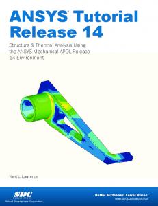
Structure & Thermal Analysis Using the ANSYS Mechanical APDL Release. 14
Environment www.SDCpublications.com. Better Textbooks. Lower Prices. SDC.
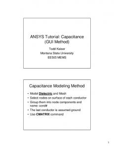
ANSYS Tutorial: Capacitance. (GUI Method). Todd Kaiser. Montana State University. EE505 MEMS. Capacitance Modeling Method. • Model Dielectric and Mesh.
Introduction to Using ANSYS FLUENT in. ANSYS Workbench: Fluid Flow and
Heat Transfer in a. Mixing Elbow. Introduction. This tutorial illustrates using
ANSYS ...
7. 2.4: Mesh Visualization and Optimization. 9. 3: ANSYS ICEM CFD GUI. 11. 3.1:
Main Menu. 12. 3.2: Utilities. 13. 3.3: Function Tabs. 13. 3.3.1: The Geometry ...
Striker. Tool made of Steel. â Assume the far face of the. Wheel/Axle is constrained. â Assume the sides of the Striker are constrained to slide up and down.
Jan 17, 2011 ... This tutorial provides instructions for creating a fluid volume and mesh around a
NACA ... 12. Insert a “#” before “NACA4314” in cell C1. The “#” is used to denote
a ... display the reason why the 3D curve was not successful. 5.
This Tutorial will use a readymade file to speed up the learning process for the ... Figure3: At the moment the illustration are a bit simplified for the user and will ...
ANSYS® Tutorial. Release 8.0 and Release 7.1. Kent L. Lawrence. Mechanical and Aerospace Engineering. University of Texas at Arlington. ______. SDC.
nucleate boiling using the in-built boiling model available under Eulerian multiphase ... In this tutorial, you will use the Eulerian multiphase model for boiling flow.
ANSYS FLUENT 13.0 Tutorial Guide, and that you are familiar with the ANSYS ... about this model, see Section 26.5, Setting Up the Eulerian Model in ANSYS ...
There was a problem previewing this document. Retrying... Download. Connect more apps... Try one of the apps below to op
required next is to press on the generate icon that is represented by a yellow thunder icon. Figure6: The DesignModeler will read in the imported data file, and ...
Postion the cursor on the mesh icon and then press the left mouse button and then ... Type the value of 30 into the U velocity input box, while for the V and W cell type in zero. ... steps then check if the required results fall into the wanted range
In this tutorial, you will model and analyze the beam below in ANSYS. ... Define element table items for plotting and listing of various stress components. 13.
Analysis software, ANSYS, for linear static, dynamic, and thermal anal- ysis through a series of ... tutorial that would supplement a course in basic finite element or can be used by practicing .... For further information, a free trial, or to order,
overhead on aggregating the load status from the nodes. We propose to apply diffusive load balancing on a clustered P2P system, where a global balance is ...
May 18, 2010 - âFluid Flow (FLUENT)â has a check mark next to it. You may need to ... The name of a toolbar button will be displayed if you hover the mouse cursor over ..... Select inlet, which is the left side of the computational domain. Edit.
ANSYS TUTORIAL. Analysis of ... In this tutorial, you will model and analyze the
beam below in ANSYS. ... Alternative Command Line Entry = r,1,8,(32/12),2,(6/5).
May 18, 2010 ... Top. Set Workbench options for a new FLUENT project. 1. This tutorial assumes
that ANSYS Workbench is running but no projects are open.
Applying a Transient Load Function. This tutorial demonstrates how to create a function in ANSYS and apply it as a pressure load for a transient analysis.
Nyquist / Haghighi
ABE 601
ANSYS Tutorial Applying a Transient Load Function This tutorial demonstrates how to create a function in ANSYS and apply it as a pressure load for a transient analysis. (Go to Main Menu) Preprocessor Element Type Add/Edit/Delete Add Structural Solid & Triangle 6node 2 & OK Close Material Props Material Models & Structural & Linear & Elastic & Isotropic & OK (Click inside the EX box) 3e7 (Click inside the NUXY box) 0.3 & OK Close Material Models window Modeling Create Areas Rectangle By Dimensions (Click X1 box) 0 (Click X2 box) 10 (Click Y1 box) 0 (Click Y2 box) 10 & OK Circle By Dimensions (Click RAD1 Box) 1 & OK
Operate Booleans Subtract Areas (Click on base area from which to subtract) Click A1 (rectangle) & Apply (Click on area to be subtracted) Click A2 (circle) & OK (GoTo Main Menu) Preprocessor Meshing MeshTool Click on the Lines SET button (Pick All) & OK (Click the SIZE box) 0.5 & OK Click the Mesh button (Pick the problem area) & OK
1
Nyquist / Haghighi
ABE 601
Solution Define Loads Apply Structural Displacement Symmetry B.C On Lines (Pick lines X=0 & Y=0 and then click) OK (Go to Utility Menu) Parameters Functions Define/Edit… (Function Editor Opens) Function Type (Choose Single Equation) Result = 5000*sin(PI/4*{TIME}) File Save Name it Load5000.func & Save Close
2
Nyquist / Haghighi
ABE 601
Parameters Functions Read from File… Select load5000.func & Open (Function loader Appears) Table Parameter Name: Sin5000 & OK
(Go to Main Menu) Solution Define Loads Apply Structural Pressure On Lines Select Line 2 & OK Apply Pressure on lines as: Choose Existing Table OK Existing Table: Click on Sin5000 & OK
3
Nyquist / Haghighi
ABE 601
Solution Analysis Type
4
Nyquist / Haghighi
ABE 601
New Analysis Choose Transient & OK Choose Full & OK Sol’n Controls Basic Tab Time at end of loadstep: 16 Click on Time Increment Time step size: 1 Frequency: Choose Write every substeps
Transient Tab Choose Ramped Loading & OK
5
Nyquist / Haghighi
ABE 601
Solve Current LS Reviewing Transient Results (Go to Main Menu) General Postproc Results Summary (16 substeps listed) Read Results By Pick (select the substep of interest) & READ Close Plot Results Contour Plot (Choose the plots of interest) (Go to Main Menu) TimeHist Postpro Time History Variables Window appears:
6
Nyquist / Haghighi
ABE 601
Add Data Button Graph Data Button
Click Add Data button Add Time-History Variable Window Appears Choose Nodal Solution Stress Von Mises & OK Choose a node on the model to examine & OK Click Graph Data button