Ant Colony Algorithm for the Unsupervised Word Sense

Ant Colony Algorithm for the Unsupervised Word Sense Disambiguation of Texts: Comparison and Evaluation Didier SCHWAB, Jérôme GOULIAN, Andon TCHECHMEDJIEV, Hervé BLANCHON LIG-Laboratory of Informatics of Grenoble GETALP-Study Group for Machine Translation and Automated Processing of Languages and Speech Univ. Grenoble-Alpes, France

{Didier.Schwab,Jerome.Goulian,Andon.Tchechmedjiev,Herve.Blanchon}@imag.fr

ABSTRACT Brute-force word sense disambiguation (WSD) algorithms based on semantic relatedness are really time consuming. We study how to perform WSD faster and better on the span of a text. Several stochastic algorithms can be used to perform Global WSD. We focus here on an Ant Colony Algorithm and compare it to two other methods (Genetic and Simulated Annealing Algorithms) in order to evaluate them on the Semeval 2007 Task 7. A comparison of the algorithms shows that the Ant Colony Algorithm is faster than the two others, and yields better results. Furthermore, the Ant Colony Algorithm coupled with a majority vote strategy reaches the level of the first sense baseline and among other systems evaluated on the same task rivals the lower performing supervised algorithms.

TITLE

AND

ABSTRACT

IN FRENCH

Algorithme à colonie de fourmis pour la désambiguïsation lexicale non supervisée de textes : comparaison et évaluation Les algorithmes exhaustifs de désambiguïsation lexicale ont une complexité exponentielle et le contexte qu’il est calculatoirement possible d’utiliser s’en trouve réduit. Il ne s’agit donc pas d’une solution viable. Nous étudions comment réaliser de la désambiguïsation lexicale plus rapidement et plus efficacement à l’échelle du texte. Nous nous intéressons ainsi à l’adaptation d’un algorithme à colonies de fourmis et nous le confrontons à d’autres méthodes issues de l’état de l’art, un algorithme génétique et un recuit simulé en les évaluant sur la tâche 7 de Semeval 2007. Une comparaison des algorithmes montre que l’algorithme à colonies de fourmis est plus rapide que les deux autres et obtiens de meilleurs résultats. De plus, cet algorithme, couplé avec un vote majoritaire atteint le niveau de la référence premier sens et rivalise avec les moins bons algorithmes supervisés sur cette tâche.

KEYWORDS: Unsupervised Word Sense Disambiguation, Semantic Relatedness, Ant Colony Algorithms, Stochastic optimization algorithms. KEYWORDS

IN FRENCH : Désambiguïsation lexicale non-supervisée, proximité sémantique, algorithmes à colonies de fourmis, algorithmes stochastiques d’optimisation

1

Introduction

Word Sense Disambiguation (WSD) is a core problem in Natural Language Processing (NLP), as it may improve many of its applications, such as multilingual information extraction, automatic summarization, or machine translation. More specifically, the aim of WSD is to find the appropriate sense(s) of each word of a text among a pre-definied sense inventory. For example, in "The mouse is eating cheese.", for the word ,mouse-, the WSD algorithm should choose the sense that corresponds to the animal rather than the computer device. There exist many methods to perform WSD, among which, one can distinguish between supervised methods and unsupervised methods. The former are based on machine learning techniques that use a set of (manually) labelled training data, whereas the latter do not. This article focusses on an unsupervised knowledge-based approach for WSD, derived from the method proposed by (Lesk, 1986). This approach uses a similarity measure that corresponds to the number of overlapping words between the definitions of two word senses. With this metric, one can select, for a given word of a text, the sense that yields the highest relatedness to a certain number of its neighbouring words (with a fixed window size). Works such as (Pedersen et al., 2005) use a brute-force (BF) global algorithm that evaluates the relatedness between each word sense and all the senses of the other words within the considered context window. The execution time is exponential in the size of the input, thus reducing the maximum possible width of the window. The problem can become intractable even on the span of short sentences: a linguistically motivated context, such as a paragraph for instance, can not be handled. Thus, such approaches can not be used for applications where real time is a necessary constraint (image retrieval, machine translation, augmented reality). In order to overcome this problem and to perform WSD faster, we are interested in other methods. In this paper, we focus on three methods that globally propagate a local algorithm based on semantic relatedness to the span of a whole text. We consider two unsupervised algorithms from the state of the art, a Genetic Algorithm (GA) (Gelbukh et al., 2003) and a Simulated Annealing (SA) algorithm (Cowie et al., 1992), as well as an adaptation of an Ant Colony Algorithm (ACA) (Schwab et al., 2011). Our aim is to provide an empirical comparison of the ACA with the two other unsupervised algorithms, using the Semeval-2007, Task-7, Coarse grained corpus (Navigli et al., 2007) (both in terms of quality and execution time). Furthermore, we also evaluate the results after applying a majority vote strategy. After a brief review of the state-of-the-art of WSD, the algorithms are described. Subsequently, their implementations are discussed, as well as the estimation of the best parameters and the evaluation of the tested algorithms. Finally, an analysis of the results is presented as well as a comparison to other systems on Semeval 2007 Task 7. Then, we conclude and propose some perspectives for future work.

2

Brief State of the art of Word Sense Disambiguation

In simple terms, WSD consists in choosing the best sense among all possible senses for all words in a text. There exist many methods to perform WSD. The reader can refer to (Ide and Véronis, 1998) for works before 1998 and (Agirre and Edmonds, 2006) or (Navigli, 2009) for a complete state of the art. Supervised WSD algorithms are based on the use of a large set of hand-labelled training data to build a classifier which can determine what are the right sense(s) for a given word in a given context. Most classical supervised learning algorithms have been applied to WSD, and

even though they tend to yield better results (on English) over unsupervised approaches, their main disadvantage is that hand-labelled examples are rare and expensive resources (knowledge acquisition bottleneck) that must be created for each sense inventory, each language and even each specialized domain. We share the opinion of (Navigli and Lapata, 2010) that unsupervised methods would be better in order to overcome these obstacles in the short term. Among unsupervised WSD methods some use raw corpora to build word vectors or cooccurrence graphs while others use external knowledge sources (dictionaries, thesauri, lexical databases, . . . ). The latter are based on the use of semantic similarity metrics that assign a score representing how related or close two word senses are. Many such measures exist and can be classified in three main categories: taxonomic distance in a lexical graph; taxonomic distance weighted by information content; feature-based similarity. More recent efforts go towards hybrid measures that combine two or more of the above. Readers may consult (Pedersen et al., 2005), (Cramer et al., 2010), (Tchechmedjiev, 2012) or (Navigli, 2009) for a more complete overview. Commonly, similarity measures use WordNet (Fellbaum, 1998), a lexical database for English widely used in the context of WSD. WordNet is organised around the notion of ”synonym sets” (synsets), which represent a word, its class (noun, verb, ...) and its connections to all semantically related words (synonyms, antonyms, hyponyms,...), as well as a textual definition for each corresponding synset. The current version, WordNet 3.0, contains over 155000 words for 117000 synsets.

3

Local and global WSD Algorithms

3.1

Our local algorithm : A variant of the Lesk Algorithm

Our local algorithm is a variant of the Lesk Algorithm (Lesk, 1986). Proposed more than 25 years ago, it is simple, only requires a dictionary and no training. The score given to a sense pair is the number of common words (space separated strings) in the definition of the senses, without taking into account neither the word order in the definitions (bag-of-words approach), nor any syntactic or morphological information. Variants of this algorithm are still today among the best on English-language texts (Ponzetto and Navigli, 2010). Our local algorithm exploits the links provided by WordNet: it considers not only the definition of a sense but also the definitions of the linked senses (using all the semantic relations from WordNet) following (Banerjee and Pedersen, 2002), henceforth referred as E x t Lesk1 . Contrarily to Banerjee, however, we do not consider the sum of squared sub-string overlaps, but merely a bag-of-words overlap that allows us to generate a dictionary from WordNet, where each word contained in any of the word sense definitions is indexed by a unique integer and where each resulting definition is sorted. Thus we are able to lower the computational complexity from O(mn) to O(m), m > n, where m and n are the respective length of two definitions. For example for the definition: "Some kind of evergreen tree", if we say that Some is indexed by 123, kind by 14, evergreen by 34, and tree by 90, then the indexed representation is {14, 34, 90, 123}.

3.2

Global algorithms

A global algorithm is a method that allows to propagate a local measure to a whole text in order to assign a sense label to each word. The simplest approach is the exhaustive evaluation of 1

All dictionaries and Java implementations of all algorithms of this article can be found on our WSD page

http://getalp.imag.fr/xwiki/bin/view/WSD/

sense combinations (BF), used for example in (Banerjee and Pedersen, 2002), that assigns a score to each word sense combination in a given context (window or whole text) and selects the one with the highest score. The main issue with this approach is that it leads to a combinatorial Q|T | explosion in the length of the context window or text: i=1 (|s(w i )|), where s(w i ) is the set of possible senses of word i of a text T . For this reason it is very difficult to use the BF approach in real-life scenarios as well as on analysis windows of more than a few words. Several approximation methods can be used in order to overcome the combinatorial explosion problem. On the one hand, complete approaches, try to reduce dimensionality using pruning techniques and sense selection heuristics. Some examples include: (Hirst and St-Onge, 1998), based on lexical chains that restrict the possible sense combinations by imposing constraints on the succession of relations in a taxonomy (e.g. WordNet); or (Gelbukh et al., 2005) that review general pruning techniques for Lesk-based algorithms; or yet (Brody and Lapata, 2008). On the other hand, incomplete approaches generally use stochastic sampling techniques to reach a local maximum by exploring as little as necessary of the search space. Our present work focuses on such approaches. Furthermore, we can distinguish two possible variants: • local neighbourhood-based approaches (new configurations are created from existing configurations) among which are some approaches from artificial intelligence such as genetic algorithms or optimization methods such as simulated annealing ; • constructive approaches (new configurations are generated by iteratively adding new elements of solutions to the configuration under construction), among which are for example ant colony algorithms.

3.3

Context of our work

The aim of this paper is to compare our Ant Colony Algorithm (incomplete and constructive approach) to other incomplete approaches. We choose to first confront our algorithm to two classical neighbourhood-based approaches that have been used in the context of unsupervised WSD: genetic algorithms (Gelbukh et al., 2003) and simulated annealing (Cowie et al., 1992). The underlying assumption to our work is that the span of the analysis context should be the whole text (similarly to (Cowie et al., 1992), (Gelbukh et al., 2003) and more recently (Navigli and Lapata, 2010)), rather than a smaller context window (like many other methods do for computational reasons). Indeed, in our opinion, using a context window smaller than that of the whole text raises two main issues: no guarantee on the consistency between two selected senses; contradictory sense assignments outside of the window range. For example in the following sentence, considering a window of 6 words: "The two planes were parallel to each other. The pilot had parked them meticulously.", plane may be disambiguated wrongly due to pilot being outside the window of plane. Furthermore it can be detrimental to the semantic unity in the disambiguation, given that as (Gale et al., 1992) or (Hirst and St-Onge, 1998) pointed out, two words used several times in the same context tend to have the same sense. Therefore, some algorithms that are similar to our Ant Colony Algorithm but that use a context window have not been studied here (notably the adaptation (Mihalcea et al., 2004) of PageRank (Brin and Page, 1998) to WSD). Moreover, we are not interested in comparing these incomplete algorithm, which cannot pragmatically be used in a real-life context, to the optimal disambiguation (Brute Force). Even with a reduced windows of the context and weeks of execution time we were only able to

achieve a 77% coverage of the corpus with BF, as detailed in (Schwab et al., 2011).

4

Global stochastic algorithms for Word Sense Disambiguation

The aim of these algorithms is to assign to each ambiguous word w i in a text of m words the most appropriate of its senses w i, j given the context. The definition of a sense j of word i is noted d(w i, j ). The search-space corresponds to all the possible sense combinations for the text being processed. Therefore, a configuration C of the problem can be represented as an array of integers such that j = C[i] is the selected sense j of w i .

4.1

Problem configuration and global score

The algorithms require some fitness measure to evaluate how good a configuration is. With this in mind, the score of the selected sense of a word can be expressed as the sum of the local scores between that sense and the selected senses of all the other words of the text. Hence, in order to obtain a fitness value (global score) for the whole configuration, it is possible to simply sum the scores for all selected senses of the words of the text: Scor e(C) = P m Pm 2 i=1 j=i E x t Lesk(w i,C[i] , w j,C[ j] ). The complexity of this algorithm is hence O(m ), where m is the number of words in the text.

4.2

Genetic algorithm for Word Sense Disambiguation

The Genetic Algorithm (GA) based on (Gelbukh et al., 2003) can be divided into five phases: initialisation, selection, crossover, mutation and evaluation. During each iteration, the algorithm goes through each phase but the initialisation. The initialisation phase consists in the generation of a random initial population of λ individuals (λ configurations of the problem). During the selection phase, the score of each individual of the current population is computed. A crossover ratio (CR) is used to determine which individuals of the current population are to be selected for crossover. The probability of an individual being selected is CR weighted by the ratio of the score of the current individual over that of the best individual. Individuals who are not selected for crossover are merely cloned (copied) into the new population. Additionally the best individual is systematically kept. After each iteration, the size of each subsequent population is a constant λ. During the crossover phase individuals are sorted according to their global score. If the number of individuals is odd, the individual with the lowest score is unselected and cloned into the new population as it cannot serve for crossover. The crossover operator is then applied on the individuals two by two in decreasing order of their score: the resulting configurations are swapped around two random pivots (everything but what is between the pivots is swapped). During the mutation phase, each individual has a probability of mutating (parameter MR, for Mutation Rate). A mutation corresponds to MN random changes in the configuration. Thus, after the mutation phase, we obtain a modified configuration Cc 0 . The evaluation phase corresponds to the test of the termination criteria: convergence of the score of the best individual. In other words if the score of the best individual remains the same for a number of generations (STH), the algorithm terminates.

4.3

Simulated annealing for Word Sense Disambiguation

The simulated annealing approach as described in (Cowie et al., 1992) is based on the physical phenomenon of metal cooling. Simulated annealing works with the same configuration representation as the genetic algorithm, however it uses a single randomly initialised configuration. The algorithm is organised in cycles and in iterations, each cycle being composed of IN iterations. The other parameters are the initial temperature T0 and the cooling rate ClR ∈ [0; 1]. At each iteration a random 0 change is made to the current configuration Cc , which results in a new configuration Cc . Given 0 0 that ∆E = Scor e(Cc ) − Scor e(Cc ), Cc , the probability P(A) of acceptance (the probability of 0 replacing Cc 0 ) of configuration Cc is : ( P(A) =

if ∆E < 0

1 e

−∆E T

otherwise

The reason why configurations with lower scores have a chance to be accepted, is to prevent the algorithm from converging on a local maximum. Lower score configurations allow to explore other parts of the search-space which may contain the global maximum. At the end of each cycle, if the current configuration is the same as the configuration at the end of the previous cycle, the algorithm terminates. Otherwise, the temperature is lowered to T · ClR. In other words, the more cycles it takes for the algorithm to converge, the lower the probability to accept lower score configurations: this guarantees an eventual convergence. The configuration with the highest score is saved after each iteration and will be taken as a result regardless of the convergence configuration.

5 5.1

Global Ant Colony Algorithm Ant Colony Algorithm

Ant colony algorithms (ACA) come from biology and from observations of ant social behavior. Indeed, these insects have the ability to collectively find the shortest path between their nest and a source of food (energy). It has been demonstrated that cooperation inside an ant colony is self-organised and emerges from interactions between individuals. These interactions are often very simple and allow the colony to solve complex problems. This phenomenon is called swarm intelligence (Bonabeau and Théraulaz, 2000) and is increasingly popular in computer science where centralised control systems are often successfully replaced by other types of control based on interactions between simple elements. Artificial ants have first been used for solving the Traveling Salesman Problem (Dorigo and Gambardella, 1997). In these algorithms, the environment is usually represented by a graph, in which virtual ants exploit pheromone trails deposited by others, or pseudo-randomly explore the graph. These algorithms are a good alternative for the resolution of problems modeled with graphs. They allow a fast and efficient exploration close to other search methods. Their main advantage is their high adaptivity to changing environments. Readers can refer to (Dorigo and Stützle, 2004), (Monmarche et al., 2009) or (Guinand and Lafourcade, 2010) for a state of the art.

5.2 5.2.1

Ant colony Algorithm for Word Sense Disambiguation Principle

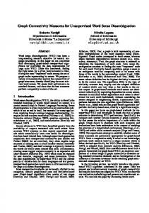
The environment of the ant colony algorithm is a graph that can be linguistic, a morphological lattice (Rouquet et al., 2010), morpho-syntactic (Schwab and Lafourcade, 2007), or simply organised following the structure of the text (Guinand and Lafourcade, 2010). Depending on the environment chosen, the results of the algorithm differ. We are currently investigating this aspect, but as the focus of our article is to make a comparison between ACA and the two other methods presented earlier, we will use a simple graph following the structure of the text (see Fig. 1) that uses no external linguistic information (no morpho-syntactic links within a sentence for example). 1

Text

2 Sentence

3 Sentence

4 Sentence

5 Word 11 Sense

6 Word

7 Word 13

12 Sense

Sense

8 Word 15

14 Sense

Sense

Word

16 Sense

9

17 Sense

10 Word 18 Sense

19 Sense

Figure 1: The environment for our experiment: text, sentences and words correspond to common nodes (1-10) and word senses to nests (11-19). In this graph, we distinguish two types of nodes: nests and plain nodes. Following (Schwab, 2005) or (Guinand and Lafourcade, 2010), each possible word sense is associated to a nest. Nests produce ants that move in the graph in order to find energy and to bring it back to their mother nest: the more energy is deposited by ants, the more ants can be produced by the nest in turn. Ants carry an odour (array) that contains the words of the definition of the sense of its mother nest. From the point of view of an ant, a node can be: (1) its mother nest, where it was born; (2) an enemy nest that corresponds to another sense of the same word; (3) a potential friend nest: any other nest; (4) a plain node: any node that is not a nest. Furthermore, to each plain node is also associated an odour vector of a fixed length that is initially empty. For example, in Fig. 1, for an ant born in nest 19: nest 18 is an enemy (as their are linked to the same word node, 10), its potential friend nodes are from 11 to 17 and common nodes are from 1 to 10. Ant movements depends on the scores given by the local algorithm (cf. Section 3.1), of the presence of energy, of the passage of other ants (when passing on an edge ants leave a pheromone trail that evaporates over time) and of the nodes’ odour vectors (ants deposit a part of their odour on the nodes they go through). When an ant arrives on a nest of another term (that corresponds to a sense thereof), it can either continue its exploration or depending on the score between this nest and its mother nest, decide to build a bridge between them and to follow it home. Bridges behave like normal edges except that if at any given time the concentration of pheromone reaches 0, the bridge collapses. Depending on the lexical information present and the structure of the graph, ants will favour

following bridges between more closely related senses. Thus, the more closely related the senses of the nests are, the more a bridge between them will contribute to their mutual reinforcement and to the sharing of resources between them (thus forming meta-nests); while the bridges between more distant senses will tend to fade away. We are thus able to build (constructive approach) interpretative paths2 through emergent behaviour and to suppress the need to use a complete graph that includes all the links between the senses from the start (as is usually the case with classical graph-based optimisation approaches). 5.2.2

Implementation details

In this section we first present the notations used (Table 1) as well as the parameters of the Ant Colony Algorithm and their typical value ranges (Table 2), followed by a detailed description of the different steps of the algorithm. Notation FA fA V (X ) E(X ) E val f (N ) E val f (A) ϕ(t/c) (A)

Description Nest that corresponds to sense A Ant born in nest FA Odour vector associated with X (ant or node) Energy on/carried by X (ant or node) Evaluation of a node N by an ant f Evaluation of an edge A (quantity of pheromone) by an ant f Quantity of pheromone on edge A at given moment t or cycle c

Table 1: Main notations for the Ant Colony Algorithm Notation Ea Ema x δ E0 ω LV δV cac

Description Energy taken by an ant when it arrives on a node Maximum quantity of energy an ant can carry Evaporation rate of the pheromone between two cycles Initial quantity of energy on each node Ant life-span Odour vector length Percentage of the odour vector components (words) deposited by an ant when it arrives on a node Number of cycles of the simulation

Value 1-30 1-60 0.0-1.0 5-60 1-30 (cycles) 20-200 0-100% 1-500

Table 2: Parameters of the Ant Colony Algorithm and their typical value-ranges 5.2.3

Simulation

The execution of the algorithm is a potentially infinite succession of cycles. After each cycle, the state of the environment can be observed and used to generate a solution. A cycle is composed of the following actions: (1) eliminate dead ants and bridges with no pheromone; (2) for each nest, potentially produce an ant; (3) for each ant: determine its mode (energy search or return); make it move; potentially create an interpretative bridge; (4) update the environment (energy levels of nodes, pheromone and odour vectors). Ant production, death and energy model Initially, we assign a fixed quantity of energy E0 to each node of the environment. At the beginning of each cycle, each nest node N has an 2

Possible interpretation of the text.

opportunity to produce an ant A using 1 unit of energy, with a probability P(NA). In accordance with (Schwab and Lafourcade, 2007) or (Guinand and Lafourcade, 2010), we define it as the following sigmoid function (often used with artificial neural networks (Lafourcade, 2011)): ar c t an(E(N )) P(NA) = + 0.5. π When created, an ant has a lifespan of ω cycles (see Table 2). When the life of an ant reaches zero, the ant is deleted at the beginning of the next cycle and the energy it carried is deposited on the node where it died. By thus doing, we ensure that the global energy equilibrium of the system is preserved, which plays a fundamental role in the convergence (monopolization of resources by certain nests) to a solution. Ant movements The ants’ movements are random, but influenced by the environment. When an ant is on a node, it assigns a transition probability to the edges leading to all neighbouring nodes. The probability to cross through an edge A j in order to reach a node Ni is P(Ni , A j ) = E val f (Ni ,A j ) Pk=n,l=m , k=1,l=1 E val f (Nk ,Al )

where E val f (N , A) = E val f (N ) + E val f (A) is the evaluation function of a

node N when coming from an edge A. A newborn ant seeks food. It is attracted by the nodes which carry the most energy (E val f (N ) = E(N ) Pm ), 0 E(Ni )

but avoids to go through edges with a lot of pheromone, E val f (A) = 1 − ϕ t (A) in

order to favour a greater exploration of the search space. The ant collects as much energy as possible until it decides to bring it back home (return mode) with the probability E( f ) P(r etur n) = E 3 . Then, it moves while following (statistically) the edges that contain the max most pheromone, E val f (A) = ϕ t (A) and leading to nodes with an odour close to their own, E val f (N ) =

E x t Lesk(V (N ),V ( fA )) Pi=k . i=1 E x t Lesk(V (Ni ),V ( f A ))

Creation, deletion and types of bridges When an ant arrives on a node adjacent to a potential friend nest (i.e. that corresponds to a sense of a word), it has to decide between taking any of the possible paths or to go on that nest node. As such, we are dealing with a particular case of the ant path selection algorithm presented above in Section 5.2.3, with E val f (A) = 0 (The pheromone on the edge is ignored). The only difference is that if the ant chooses to go on the potential friend nest, a bridge between that nest and the ant’s home nest is built and the ant follows it to go home. Bridges behave like regular edges, except that if the concentration of pheromone on them reaches 0, they collapse and are removed. Pheromone Model Ants have two types of behaviours: they are either looking to gather energy or to return to their mother nest. When they move in the graph, they leave pheromone trails on the edges they pass through. The pheromone density on an edge influences the movements of the ants: they prefer to avoid edges with a lot of pheromone when they are seeking energy and to follow them when they want to bring the energy back to their mother nest. When passing on an edge A, ants leave a trail by depositing a quantity of pheromone θ ∈ IR+ such that ϕ t+1 (A) = ϕ t (A) + θ . Furthermore, at each cycle, there is a slight (linear) evaporation of pheromones (penalizing little frequented paths). Thus, ϕ t+1 (A) = ϕ t (A)×(1−δ), where δ is the pheromone evaporation rate. 3

Consequently, when the ant reaches its carrying capacity, the probability to switch to return mode is 1.

Odour The odour of a nest is the numerical sense vector (as introduced in Section 3.1) and corresponds to the definition of the sense associated to the nest. All ants born in the same nest have the same odour vector. When an ant arrives on a common node N , it deposits some of the components of its odour vector (following a uniform distribution), which will be added to or will replace existing component of the node’s vector V (N ). The odour of nest nodes on the other hand is never modified. This mechanism allows ants to find their way back to their mother nest. Indeed, the closer a node is to a given nest, the more ants from that nest will have passed through and deposited odour components. Thus, the odour of that node will reflect its nest neighbourhood and allow ants to find their way by computing the score between their odour (that of their mother nest) and the surrounding nodes and by choosing to go on the node yielding the highest score. This process leaves some room for error (such as an ant arriving on a nest other than its own), which is beneficial as it leads ants to build more bridges (see Section 5.2.3).

5.3

Global Evaluation

At the end of each cycle, we build the current problem configuration from the graph: for each word, we take the sense corresponding to the nest with the highest quantity of energy. Subsequently, we compute the global score of the configuration (see Section 4.1). Over the execution of the algorithm we keep the configuration with the highest absolute score, which will be used at the end to generate the solution.

5.4

Main parameters

Here we present a short characterisation of the influence of the parameters on the emergent phenomena in the system: • The maximum amount of energy an ant can carry, Emax , influences how much an ant explores the environment. Ants cannot go back through an edge they just crossed and have to make circuits to come back to their nest (if the ant does not die before that). The size of the circuits depend on the moment the ants switch to return mode, hence on Emax . • The evaporation rate of the pheromone between cycles (δ) is one of the memories of the system. The higher the rate is, the least the trails from previous ants are given importance and the faster interpretative paths have to be confirmed (passed on) by new ants in order not to be forgotten by the system. • The initial amount of energy per node (E0 ) and the ant life-span (ω) influence the number of ants that can be produced and therefore the probability of reinforcing less likely paths. • The odour vector length (L v ) and the proportion of odour components deposited by an ant on a plain node (δV ) are two dependent parameters that influence the global system memory. The higher the length of the vector, the longer the memory of the passage of an ant is kept. On the other hand, the proportion of odour components deposited has the inverse effect. Given the lack of an analytical way of determining the optimal parameters of both the Ant Colony Algorithm and the other algorithms presented, they have to be estimated experimentally, which is detailed in Section 6.

6

Empirical Evaluation

In this section we first describe the evaluation task we used to evaluate the three systems, followed by the methodology we used for the estimation of the parameters, and then the experimental protocol for the empirical quantitative comparison of the algorithms and subsequently, the interpretation of the results. Finally, we briefly compare the number of evaluations of the semantic similarity score function (E x t Lesk) and discuss the positioning of our system relatively to the other systems that are evaluated with Semeval 2007 Task 7 (participating systems and more recent advances).

6.1

Evaluation Campaign Task

We evaluated the algorithms with the SemEval 2007 coarse-grained English all-words task 7 corpus (Navigli et al., 2007). Composed of 5 texts from various domains (journalism, book review, travel, computer science, biography), the task consists in annotating 2269 words with one of their possible senses from WordNet, with an average degree of polysemy of 6.19. The evaluation of the output of the algorithm is done considering coarse grained senses distinction i.e. close senses are counted as equivalent (e.g. snow/precipitation and snow/cover). A Perl script that evaluates the quality of the solutions is provided with the task files and allows us to compute the Precision, Recall, and F1 score4 , which are the standard measures for evaluating WSD algorithms (Navigli, 2009).

6.2

Parameter estimation

The algorithms we are interested in have a certain number of parameters that need tuning in order to obtain the best possible score on the evaluation corpus. There are three approaches: • Make an educated guess about the value ranges based on a priori knowledge about the dynamics of the algorithm; • Test manually (or semi-manually) several combinations of parameters that appear promising and determine the influence of making small adjustments to the values ; • Use a learning algorithm on a subset of the evaluation corpus, for example with SA or GA to find the parameters that lead to the best score. Both GA and SA, as presented in (Gelbukh et al., 2003) and (Cowie et al., 1992) respectively, use the Lesk semantic similarity measure as a score metric. We reimplemented them with the E x t Lesk measure and used the optimal parameters provided. However, the similarity values are higher than with the standard Lesk algorithm and we had to adapt the parameters to reflect that difference. We made one parameter vary at a time over 10 executions, in order to maximise the F1 measure. For our ACA, given that an execution of the algorithm is very fast5 , it was possible to use a simplified simulated annealing approach for the automated estimation of the parameters. For each parameter combination we ran the algorithm 50 times and considered the means coupled with the p-values from a one-way ANOVA. We still needed to use our a priori knowledge to set likely parameter intervals and discreet steps for each of them6 . The best parameters we found are: 4

F1 is the harmonic mean of P and R. When 100% of the corpus is annotated, P = R = F1 . Depending on the parameters the execution takes between 15s to 40s for the first text of the corpus. 6 Supervised approach to parameter tuning which does not affect the unsupervised nature of the algorithm itself. 5

• For GA: λ = 500, CR = 0.9, M R = 0.15, M N = 80, CR = 0.9; • For SA: T0 = 1000, C lR = 0.9, I N = 1000; • For ACA: ω = 25, Ea = 16, Emax = 56, E0 = 30, δ v = 0.9, δ = 0.9, L V = 100

6.3

Experimental Protocol

The objective of the experiments is to compare the three algorithms according to different criteria. First, the F1 score obtained on the Task 7 of Semeval 2007 and then the execution time. Furthermore, given that they use the same similarity measure and that it is the computational bottleneck, we also measure the average number of similarity computations between word senses. Since the algorithms are stochastic, we need to have a representation of the distribution of solutions as accurate as possible in order to make statistically significant comparisons and thus we ran the algorithms 100 times each. The first step in the evaluation of the significance of the results is the choice of an appropriate statistical tool. In this case we are using a one-way ANOVA analysis (Miller, 1997), coupled with a Tuckey’ HSD post-hoc pairwise analysis (Hsu, 1996). These two techniques rely on three principal assumption: independence of the groups, normal distribution of the samples, within group homegeneity of variances. After the direct comparison of the results we apply a majority voting strategy for each word among ten consecutive executions so as to obtains 100 overlapping vote results. The same evaluation methodology is applied. In both cases, the baseline for our comparison is the first-sense(FS) baseline. Let us now check for the ANOVA assumptions and analyse the results.

6.4

Quantitative results

In order to check the normality assumption for ANOVA, we computed the correlation between the theoretical (normal distribution) and the empirical quantiles. For all metrics and algorithms there was always a correlation above 0.99. Furthermore we used Levene’s variance homogeneity test and found a minimum significance level of 10−6 between all algorithms and metrics. Algorithm

F1 (%)

σ F1

T ime(s)

σ T ime

Sim. Eval.

σ(S.E v.)

F.S. Baseline G.A. S.A. A.C.A.

77.59 73.98(74.53)† 74.23(75.18)† 76.41(77.50)†

N/A 0.0052 0.0028 0.0048

N/A 4,537.6† 1,436.6† 65.46†

N/A 963.2 167.3 0.199

N/A 137,158,739† 4,405,304† 1,559,049†

N/A 13,784.43 50,805.27 17,482.45

Table 3: Comparison of the F1 scores (after vote between brackets), execution times and similarity measure evaluations of the algorithms († ↔ p < 0.01) over texts 2 through 5. Table 3 presents the results, for the three algorithms with the F1 scores, execution time and number of evaluations of the similarity measure along with their respective standard deviations. For all three metrics and between all three algorithms, the difference in the means was systematically significant with p