Ant Colony Optimization with Partial Order Reduction for Discovering Safety Property Violations in Concurrent Models ? Francisco Chicano ∗ , Enrique Alba Departamento de Lenguajes y Ciencias de la Computaci´ on University of M´ alaga, SPAIN
Abstract In this article we analyze the combination of ACOhg, a new metaheuristic algorithm, plus partial order reduction applied to the problem of finding safety property violations in concurrent models using a model checking approach. ACOhg is a new kind of ant colony optimization algorithm inspired by the foraging behaviour of real ants equipped with internal resorts to search in very large search landscapes. We here apply ACOhg to concurrent models in scenarios located near the edge of the existing knowledge in detecting property violations. The results state that the combination is computationally beneficial for the search and represents a considerable step forward in this field with respect to exact and other heuristic techniques. Key words: Program correctness, ant colony optimization, metaheuristics, model checking, HSF-SPIN
1. Introduction From the very beginning of computer research, computer engineers have been interested in techniques allowing them to know if a software module fulfils a set of requirements (its specification). These techniques are especially important in critical software, such as airplane, nuclear plants, and spacecraft software controllers, in which people’s lives depend on the software system. In addition, modern non-critical software (like communication protocols) is very complex and these techniques have become a necessity in most software companies. Model checking [8] is a well-known and fully automatic formal method in which all the possible states of a given model are analyzed (in an explicit or implicit way) in order to prove (or refute) that the model satisfies a given property. This property is specified using a temporal logic like Linear Temporal Logic (LTL) or Computation Tree Logic (CTL). In a recent work [3], a new kind of ant colony optimization algorithm called ACOhg was applied to the problem of
finding safety property violations in concurrent models using a model-checking based approach. The new algorithm is able to get short error paths (good quality solutions) with a low amount of memory in all the studied models. The contribution of the present work is to combine ACOhg with a technique for reducing the memory consumption of the algorithm: partial order reduction [14]. With this combination we expect to reduce even more the amount of computational resources required by ACOhg to find execution error paths in concurrent models. This is a very important step forward in software engineering, since it allows the construction of efficient tools for checking real software. This article is organized as follows. In the next section, we present the background and related work. Section 3 formalizes the problem at hands and describes both the ACOhg algorithm and the partial order reduction. In Section 4 we apply ACOhg with and without partial order reduction and analyze the results. Finally, Section 5 summarizes our conclusions and future work. 2. Background
? This work has been partially funded by the Ministry of Education and Science and FEDER under contract TIN2005-08818-C04-01 (the OPLINK project). Francisco Chicano is supported by a grant (BOJA 68/2003) from the Junta de Andaluc´ıa. ∗ Corresponding author. Email addresses:
[email protected] (Francisco Chicano),
[email protected] (Enrique Alba). Preprint submitted to Elsevier
Our proposal is based on explicit state model checking. One of the best known explicit state model checkers is SPIN [19], which takes a software model codified in Promela and a property specified in LTL as inputs. SPIN transforms the model and the negation of the LTL formula into B¨ uchi 22 November 2007
automata in order to perform their intersection. The resulting intersection automaton is explored to search for a path starting in the initial state and including a cycle of states containing an accepting state. If such a path is found, then there exists at least one execution of the model not fulfilling the LTL property (see [19] for more details). If such kind of path does not exist, then the model fulfils the property and the verification ends with success. In SPIN this exploration is performed with Nested-DFS [20], an exhaustive algorithm. When the property to check is a safety property [23], the verification is reduced to a search for one path from the initial state to one accepting state in the B¨ uchi automaton. This path represents an execution of the concurrent model in which the given safety property is violated. Finding such a path is the case in which we are interested. The amount of states of the intersection automaton is very high even in the case of small models, and it increases exponentially with their size. This fact is known as the state explosion problem and limits the size of the model that a model checker can verify. This limit is reached when it is not able to explore more states due to the absence of free computer memory. Several techniques exist to alleviate this problem. They aim at reducing the amount of memory required for the search by following different approaches. On the one hand, there are techniques which reduce the number of states to explore, such as partial order reduction [22] or symmetry reduction [21]. On the other hand, techniques exist that reduce the memory required for storing one state, such as state compression, minimal automaton representation of reachable states, and bitstate hashing [19]. In spite of the fact that they are largely used, exhaustive search techniques such as Nested-DFS are always handicapped since real concurrent programs are too complex even for the most advanced techniques. In the first stages of the software development, when the probability of finding errors in the software is high, a good practice consists in guiding this exhaustive search by means of heuristics to gain in efficiency when searching for errors. The utilization of heuristics in model checking is well known and called heuristic or directed model checking. The heuristics are designed to explore first the region of the state space in which an error is likely to be found. This way, the time and memory required to find an error in faulty concurrent models is reduced on average. However, no benefit from heuristics is obtained when the goal is to verify that a given model fulfils a given property. In this case, the state space must be explored exhaustively. Exhaustive algorithms using heuristics, such as A∗ or Best First (BF), can find errors in models by using less resources than non-heuristic exhaustive approaches like Depth First Search (DFS) and Breadth First Search (BFS) and, in addition, they can verify the model if no error exists (since they are exhaustive algorithms) [11]. However, when the search for errors with a very low amount of computational resources (memory and time) is a priority, non-exhaustive algorithms using heuristic information can be used. One example of this class of algorithms is Beam-search, included in
the Java PathFinder model checker [16,17]. Non-exhaustive algorithms have been shown to find errors in programs using less computational resources than exhaustive algorithms [2,3]. A well-known class of non-exhaustive algorithms for solving general complex problems is the class of metaheuristic algorithms [6]. They are search algorithms used in global optimization problems which can find good quality solutions in a reasonable time. The search for accepting states in a B¨ uchi automaton can be translated into an optimization problem and, thus, metaheuristic algorithms can be applied. In fact, Genetic Algorithms (GA), a kind of metaheuristic algorithm, have been applied in the past to the search for errors in concurrent programs. In an early proposal, Alba and Troya [5] used GAs for detecting errors (deadlocks, useless states, and useless transitions) in communication protocols. To the best of our knowledge, this is the first application of a metaheuristic algorithm to the problem of finding errors in concurrent models using a model-checking based approach. Later, Godefroid and Kurshid [15], in an independent work, applied also GAs to the same problem. In [1], Alba and Chicano presented a new kind of Ant Colony Optimization (ACO) algorithm called ACOhg that is able to deal with very large construction graphs. Unlike GA, ACO is a metaheuristic designed for searching short paths in graphs. This makes it very suitable for the problem of searching for safety property violations in concurrent models. In fact, the results obtained were very impressive. ACOhg was able to find short counterexamples using a very low amount of resources, outperforming, in general, exhaustive algorithms that are the state-of-the-art in model checking [3]. Although it is not the first time that an ACO-like algorithm is applied to a problem in the software engineering domain [9], ACOhg is a novel contribution in the context of Search-Based Software Engineering [18]. Our goal here is to still improve ACOhg by including partial order reduction, a technique coming from traditional model checking. 3. Details of the Proposal In this section we first formalize the problem and then we describe the ACOhg algorithm and the partial order reduction technique. 3.1. Problem Formalization The problem of searching for safety property violations can be translated into the search of a path in a graph (the intersection B¨ uchi automaton) starting in the initial state and ending in an objective node (accepting state). We formalize here the problem as follows. Let G = (S, T ) be a directed graph where S is the set of nodes and T ⊆ S × S is the set of arcs. Let q ∈ S be the initial node of the graph and F ⊆ S a set of distinguished 2
nodes that we call final nodes. We denote with T (s) the successors of node s. A finite path over the graph is a sequence of nodes π = s1 s2 . . . sn where si ∈ S for i = 1, 2, . . . , n. We denote with πi the ith node of the sequence and we use |π| to refer to the length of the path, that is, the number of nodes of π. We say that a path π is a starting path if the first node of the path is the initial node of the graph, that is, π1 = q. We will use π∗ to refer to the last node of the sequence π, that is, π∗ = π|π| . Given a directed graph G the problem at hands consists in finding a starting path π ending in a final node. That is, find π subject to π1 = q ∧ π∗ ∈ F . The graph G used in the problem is derived from the intersection B¨ uchi automaton B of the model and the negation of the LTL formula of the property. The set of nodes S in G is the set of states in B, the set of arcs T in G is the set of transitions in B, the initial node q in G is the initial state in B, and the set of final nodes F in G is the set of accepting states in B. In the following, we will also use the words state, transition, and accepting state to refer to the elements in S, T , and F , respectively.
a given number of steps σs (called stage). If no objective node is found, the last nodes of the best paths constructed by the ants are used as starting nodes for the ants in the next stage. In this way, during the next stage the ants try to go further in the graph (see [3] for more details). In Algorithm 1 we present the pseudocode of ACOhg. Algorithm 1 ACOhg algorithm 1: init ← {q}; 2: next init ← ∅; 3: τ ← initialize pheromone(); 4: step ← 1; 5: stage ← 1; 6: while step ≤ msteps ∧ @i ∈ [1..colsize] • ai∗ ∈ F do 7: for k = 1 to colsize do {Ant operations} 8: ak ← ∅; 9: ak1 ← select init node randomly(init); 10: while |ak | ≤ λant ∧ T (ak∗ ) − ak 6= ∅ ∧ ak∗ ∈ / F do 11: node ← select successor(ak∗ , T (ak∗ ), τ, η); ak ← ak + node; 12: 13: τ ← local pheromone update(τ, ξ, (ak∗ , node)); 14: end while 15: next init ← select best paths(init, next init, ak ); 16: if f (ak ) < f (abest ) then 17: abest ← ak ; 18: end if 19: end for τ ← pheromone evaporation(τ, ρ); 20: 21: τ ← pheromone update(τ, abest ); 22: if step ≡ 0 mod σs then 23: init ← next init; 24: next init ← ∅; 25: stage ← stage + 1; 26: τ ← pheromone reset(); 27: end if 28: step ← step + 1; 29: end while
3.2. ACOhg Algorithm ACOhg is a new kind of Ant Colony Optimization model proposed by Alba and Chicano [3] that can deal with construction graphs of unknown size or too large to fit into the computer memory. Actually, this new model was proposed for applying an ACO-like algorithm to the problem of searching for counterexamples of safety properties in very large concurrent models. The objective of the algorithm is to solve the problem described in the previous section. ACO metaheuristic [10] is a global optimization algorithm inspired by the foraging behaviour of real ants. The main idea consists in simulating the ants behaviour in a graph, called construction graph, in order to search for the shortest path from an initial node to an objective one. The cooperation among the different simulated ants is a key factor in the search that is performed indirectly by means of pheromone trails, which is a model of the chemicals real ants use for their communication. The main procedures of an ACO algorithm are the construction phase and the pheromone update. These two procedures are scheduled during the execution of ACO until a given stopping criterion is fulfilled. In the construction phase, each artificial ant follows a path in the construction graph. In the pheromone update, the pheromone trails of the arcs are modified. In short, the two main differences between ACOhg and the traditional ACO models are the following ones. First, the length of the paths (defined as the number of arcs in the path) traversed by ants in the construction phase is limited. That is, when the path of an ant reaches a given maximum length λant the ant is stopped. Second, the ants start the path construction from different nodes during the search. At the beginning, the ants are placed on the initial node of the graph, and the algorithm is executed during
In the following we will describe the algorithm, but previously we are going to clarify some issues related to the notation used in Algorithm 1. In the pseudocode, the path traversed by the kth artificial ant is denoted with ak . For this reason we use the same notation as in Section 3.1 for referring to the length of the path (|ak |), the jth node of the path (akj ), and the last node of the path (ak∗ ). We use the operator + to refer to the concatenation of two paths. In line 10, we use the expression T (ak∗ ) − ak to refer to the elements of T (ak∗ ) that are not in the sequence ak . That is, in that expression we interpret ak as a set of nodes. The set init contains starting paths and next init is the set of the best paths found in one stage. The value of the variable stage does not affect the behaviour of the algorithm, we just included it to clearly mark when there is a change of stage. As in all metaheuristics, in order to guide the search, an objective function that assigns a real value to each path (reporting its quality) is used: the fitness function, which is 3
denoted with f . In our case, the fitness function is defined as follows |π + ak | if ak∗ ∈ F f (ak ) =
k |π + ak | + h(ak∗ ) + pp + pc λant − |a | if ak∗ ∈/ F ,
(1)
Pheromone Trail
IJij
λant − 1
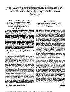
where π is the starting path in init whose last node is the first one of ak , pp , and pc are penalty values that are added when the ant does not end in a final node and when ak contains a cycle, respectively. The last term in the second row of Eq. (1) makes the penalty higher in shorter cycles. The intuition behind this is that longer cycles are nearer of a path without a cycle. For this reason we add the maximum cycle penalty (pc ) when the ant length is the minimum (|ak | = 1) and no cycle penalty is added when there is no cycle (|ak | = λant ). The function h is the so-called heuristic function, which assigns a heuristic value to each state. This heuristic value is a lower bound of the number of transitions required to get an accepting state. This function depends on the property to check and, for this reason, we defer its definition to the experimental section. The algorithm works as follows. At the beginning, the variables are initialized (lines 1-5). All the pheromone trails are initialized with the same value: a random number between 0.1 and 10. In the init set, a starting path with only the initial node is inserted (line 1). This way, all the ants of the first stage begin the construction of their path at the initial node. After the initialization, the algorithm enters in a loop that is executed until a given maximum number of steps is performed or an ant reaches a final node (line 6). In a loop, each ant builds a path starting in the final node of a previous path (line 9). This path is randomly selected from the init set using a fitness proportional probability distribution. For the construction of the path, the ants enter a loop (lines 1014) in which each ant k stochastically selects the next node according to the pheromone (τij ) and the heuristic value (ηij ) associated to each arc (i, j) whose tail is ak∗ (line 11). In particular, if the last node of the kth ant path is i = ak∗ , then the ant selects the next node j ∈ T (i) with probability [τij ]α [ηij ]β , for j ∈ T (i) , α β s∈T (i) [τis ] [ηis ]
pkij = P
k
Heuristic
i
Șij
T(i) n
j m l
Fig. 1. An ant during the construction phase.
it is defined in the context of ACO algorithms. It is a nonnegative function used by ACO algorithms for guiding the search. The higher the value of ηij , the higher the probability of selecting arc (i, j) during the construction phase of the ants. The second heuristic, h, depends on each state of the B¨ uchi automaton and it is defined in the context of the problem (heuristic model checking). This heuristic is a nonnegative function designed to be minimized, that is, the lower the value of h(j), the higher the preference to explore node j. In order to search for safety property violations using ACOhg we must define η after h. The exact expression we use is ηij = 1/(1 + h(j)). This way, ηij increases when h(j) decreases (high preference to explore node j). The pheromone trail associated to the arc (i, j) = (antk∗ , node) that the ant traverses is updated during the construction phase (line 13) using the expression τij ← (1 − ξ)τij ,
(3)
where ξ, with 0 < ξ < 1, controls the evaporation of the pheromone during the construction phase. This mechanism increases the exploration of the algorithm, since it reduces the probability that an ant follows the path of a previous ant in the same step. All this construction phase is iterated until the ant reaches the maximum length λant , it finds a final node, or all the successors of the last node of the current path, T (ak∗ ), have been visited by the ant during the construction phase. This last condition prevents the ants from constructing cycles in their paths. However, cycles can exist in the paths ending in an accepting state if more than one stage is required to find it. The reason is that ant ak does not check if the appended nodes are included in the starting path π of init which ak extends. In spite of this, ACOhg favors short paths during the search and this fact helps the algorithm to find error paths without cycles. After the construction phase, the ant is used to update the next init set (line 15), which will be the init set in the next stage. In next init, only starting paths are allowed and all the paths must have different last nodes (this is ensured by select best paths). A path ak is inserted in this set if its last node is not one of the last nodes of a starting
(2)
where α and β are two parameters of the algorithm determining the relative influence of the pheromone trail and the heuristic value on the path construction, respectively (see Fig. 1). According to the previous expression, artificial ants prefer paths with a higher concentration of pheromone, like real ants in real world. When an ant has to select a node, the last node of the current ant path is expanded. Then the ant selects one successor node and the remaining ones are removed from memory. This way, the amount of memory required in the path construction is small. At this moment we must talk about the two heuristic functions presented before: η and h. The heuristic function η depends on each arc of the construction graph and 4
path π already included in the set. If this does not hold, the new path ak replaces the starting path π of next init only if f (ak ) < f (π). Before the inclusion, the path must be concatenated with the corresponding starting path of init, that is, the starting path π with π∗ = ak1 (this path exists and it is unique). This way, only starting paths are stored in the next init set. The cardinality of next init is bounded by a given parameter ι. When this limit is reached and a new path must be included in the set, the starting path with higher fitness value is removed from the set. When all the ants have built their paths, a pheromone update phase is performed. First, all the pheromone trails are reduced, simulating the real world evaporation of pheromone trails, according to the expression τij ← (1 − ρ)τij (line 20), where ρ is the pheromone evaporation rate and it holds that 0 < ρ ≤ 1. Then, the pheromone trails associated to the arcs traversed by the best-so-far ant (abest ) are increased (line 21) using the expression τij ← τij +
1 , ∀(i, j) ∈ abest . f (abest )
concurrent models imposes an arbitrary ordering between concurrent events. When the B¨ uchi automaton of the system is built, the events are interleaved in all possible ways. The ordering between independent concurrent instructions is meaningless. Hence, we can consider just one ordering for checking one given property since the other orderings are equivalent. This fact can be used to construct a reduced state graph hopefully much easier to explore compared to the full state graph (original B¨ uchi automaton). We use here a POR proposal based on ample sets [22]. Before giving more details on POR, we need to introduce some terminology. We call transition to a partial function γ : S → S. Intuitively, a transition corresponds to one instruction in the program code of the concurrent model. The set of all the transitions that are defined for state s is denoted with enabled(s). According to these definitions, the set of successors of s must be T (s) = {γ(s)|γ ∈ enabled(s)}. In short, we say that two transitions γ and δ are independent when they do not disable one another and executing them in either order results in the same state. That is, for all s if γ, δ ∈ enabled(s) it holds that: (i) γ ∈ enabled(δ(s)) and δ ∈ enabled(γ(s)) (ii) γ(δ(s)) = δ(γ(s)) Let L : S → 2AP be a function that labels each state of the B¨ uchi automaton B with a set of atomic propositions from AP . In the B¨ uchi automaton of a concurrent system, this function assigns to each state s the set of propositions appearing in the LTL formula that are true in s. One transition γ is invisible with respect to a set of propositions AP 0 ⊆ AP when its execution from any state does not change the value of the propositional variables in AP 0 , that is, for each state s in which γ is defined, L(s) ∩ AP 0 = L(γ(s)) ∩ AP 0 . The main idea of ample sets is to explore only a subset ample(s) ⊆ enabled(s) of the enabled transitions of each state s such that the reduced state space is equivalent to the full state space. This reduction of the state space is performed on-the-fly while the graph is generated. In order to keep the equivalence between the complete and the reduced B¨ uchi automaton, the reduced set of transitions must fulfil the following conditions [8]: – C0: for each state s, ample(s) = ∅ if and only if enabled(s) = ∅. – C1: for all state s and all path in the full state graph that starts at s, a transition γ that is dependent on a transition δ ∈ ample(s) cannot be executed without a transition in ample(s) occurring previously. – C2: for all state s, if enabled(s) 6= ample(s) then all transition γ ∈ ample(s) is invisible with respect to the atomic propositions of the LTL formula being verified. – C3: a cycle is not allowed if it contains a state in which some transition γ is enabled but never included in ample(s) for any state s of the cycle. The first three conditions are not related to the particular search algorithm being used. However, the way of ensuring C3 depends on the search algorithm. In [22] three alternatives for ensuring that C3 is fulfilled were proposed. From them, the only one that can be applied to any possi-
(4)
This way, the best path found is awarded with an extra amount of pheromone and the ants will follow that path with higher probability in the next step, as in real world. We use here the mechanism introduced in Max-Min Ant Systems (MMAS) for keeping the value of pheromone trails in a given interval [τmin , τmax ] in order to maintain the probability of selecting one node above a given threshold. The values of the trail limits are 1 , (5) ρf (abest ) τmax τmin = , (6) a where the parameter a controls the size of the interval. When one pheromone trail is greater than τmax it is set to τmax and, in a similar way, when it is lower than τmin it is set to τmin . Each time that abest is updated, the interval limits are updated consequently, and all pheromone trails are checked in order to keep them inside the interval. Finally, with a frequency of σs steps, a new stage starts. The init set is replaced by next init and all the pheromone trails are removed from memory (lines 22-27). In addition to the pheromone trails, the arcs to which the removed pheromone trails are associated are also discarded (unless they also belong to a path in next init). This removing step allows the algorithm to reduce to a minimum value the amount of memory required. This minimum amount of memory is the one utilized for storing the best paths found in one stage (the next init set). τmax =
3.3. Partial Order Reduction Partial order reduction (POR) is a method that exploits the commutativity of asynchronous systems in order to reduce the size of the state space. The interleaving model in 5
ble exploration algorithm is the so-called C3static and this is the one we use in our experiments. In order to fulfil condition C3static , the structure of the processes of the model is statically analyzed and at least one transition on each local cycle is marked as sticky. Condition C3static requires that states s containing a sticky transition in enabled(s) be fully expanded: ample(s) = enabled(s). This condition is also called c2s in a later work by Boˇsnaˇcki et al. [7].
our experiments we use much larger models. In fact, the smaller ones used in our work are leader6, giop21, and marriers10, while the larger ones are leader10, giop61, and marriers20. 4.2. Parameters of the Algorithms We use two algorithms for the experiments: ACOhg and ACOhgP OR , the combination of ACOhg plus POR. The parameters used for the two algorithms are the ones shown in Table 1. These parameters are not set in an arbitrary way: they are the result of a previous study aimed at finding the best configuration for them. One portion of this study was published in [1]. Since we are working with stochastic algorithms, we need to perform several independent runs in order to get quantitative information of the behaviour of the algorithm. For this reason we perform 100 independent runs to get a high statistical confidence, and we report the mean and the standard deviation of the independent runs. The heuristic function h used is the one that assigns to each state s the number of active processes in the state (for giop and marriers) and a formula-based heuristic hϕ [13] (in the case of leader). The machine used in the experiments is a Pentium 4 at 2.8 GHz with 512 MB of RAM.
4. Experimental Section In this section we are going to analyze how the combination of partial order reduction plus ACOhg can help in the search for safety property violations in concurrent models. For the experiments we implemented the ACOhg algorithm in C++ inside the MALLBA library for metaheuristics [4]. This implementation of ACOhg is very general and thus it can be readily applied to other combinatorial optimization problems. In order to apply ACOhg to the problem at hands we included the previous implementation of ACOhg inside one model checker: HSF-SPIN. This model checker is an extension by Leue, Edelkamp, and Lluch-Lafuente of the well known SPIN model checker [19]. HSF-SPIN was developed as an experimental model checker for exploring heuristic model checking [11]. For this reason HSF-SPIN includes a set of heuristic functions defined by Edelkamp et al. [12].
Table 1 Parameters for ACOhg and ACOhgP OR . Parameter
4.1. Promela Models We apply our algorithms to a benchmark of concurrent models codified in Promela [19]. In fact, we have selected three scalable models used by Edelkamp et al. [22] in the past: giop, leader, and marriers. The first model, giop, is an implementation of the CORBA Inter-ORB protocol. The second model, leader, is a leader election algorithm for a unidirectional ring. The last model, marriers, is a protocol solving the stable marriage problem. The model giop has two parameters that allow us to generate an instance of the model as large as we want: the number of clients and the number of servers. We will denote with giopij an instance of the model with i clients and j servers (j can only be 1 or 2). The other two models have one parameter: the number of suitors, in the case of marriers, and the number of processes involved in the election, in the case of leader. The three models violate a safety property: deadlock in the case of giop and marriers and one assertion in the case of leader. The Promela source code of all these models can be found along with the modified version of HSF-SPIN in http://oplink.lcc.uma.es/software. The previous models have been used in the work by Lluch-Lafuente et al. [22] for analyzing the POR technique with A∗ . In the cited work, the scaled models used are leader5, giop21, and marriers3. As the authors state in [22], these scaled models are the larger ones that fit (fully expanded) into 512 MB of computer memory. In
Value
Parameter
Value
msteps
1000
a
5
colsize
10
ρ
0.2
λant
20
α
1.0
σs
4
β
ι
10
pp
1000
2.0
ξ
0.5
pc
1000
4.3. Results In Table 2 we present the results of applying ACOhg and ACOhgP OR to nine models: three instances of each scalable model presented above (small, medium, and large). The information reported is the length of the error paths, the memory required (in Kilobytes), the number of expanded states during the search, and the CPU time required (in milliseconds). Even though ACOhg and ACOhgP OR could fail to find an error path in theory, this never happened in practice in any of the 9 × 100 runs of each algorithm (100% of success). This statement becomes important if we take into account that the models used in the experiments are very large. In order to clarify that the reduced amount of memory required by the ACOhg algorithms is not due to the use of the heuristic information (h), we also show the results obtained with A∗ (implemented in HSF-SPIN) for all the models using the same heuristic functions as the ACOhg algorithms. This clearly states that memory reduction is a very appealing attribute of the algorithm itself. 6
Table 2 Results (mean and standard deviation values) of ACOhg and ACOhgP OR (bold values represent best results). We also include the results obtained with A∗ .
50.90
40.46
-
13.43
61.74
3.16
-
473.59
11591.68
477.67
-
597.36
2398.55
378.58
-
71.02
391.70
43.86
-
3.04
37.00
494.39
3710.64
410.29
132096.00
Exp. states 1894.28
22.38
1955.23
82.64
21332.00
21.12
98.80
8.16
1250.00
4.66
74.11
4.51
-
515.98
4831.40
114.10
-
320.90
2749.75
12.29
-
211.47
198.90
4.67
-
4.79
80.86
6.36
-
7178.05 2225.78
-
CPU (ms)
494.00
Length
60.83
Mem. (KB) 24381.44 Exp. states 2344.63 1061.20 73.84
Mem. (KB) 30167.04 Exp. states 2764.42 CPU (ms)
1910.70 307.11
Mem. (KB) 34170.88
586.82 53.06
3114.22
45.02
294.90
34.87
233.19
494.39
18319.36
315.07
70000
66.96
-
60000
21.91
-
50000
804.93
Exp. states 12667.11 1420.18
9614.15 1032.06
-
CPU (ms)
8847.00
634.06
1306.60
126.56
-
540.41
60.88
395.10
40.07
-
Mem. (KB) 51148.80
223.18
26050.56 1256.81
-
Exp. states 22506.36 2526.52 16458.42 1671.93
-
CPU (ms) 19740.50 1935.54
3595.00
316.59
-
569.99
54.63
-
33351.68 1442.75
-
Exp. states 33108.85 3364.88 23747.43 2309.39
-
CPU (ms) 49446.30 7557.40
-
Length
793.62
80.45
Mem. (KB) 68003.84
503.64
8174.00
ACOhg-h
-
-
Length
marriers20
42.39
4.52
Length
marriers15
-
Mem. (KB) 16005.12
Length
marriers10
363.91
264.90
56.36
CPU (ms)
leader10
325.19
707.71
ACOhg-h+POR
40000 30000 20000 10000 0 m ar rie rs 20
Length
-
m ar rie rs 15
440.60
422.94
2347.94
er 10 m ar rie rs 10
CPU (ms)
331.76
8
2603.47
-
ad
leader8
Exp. states
5.79
7420.08
er
leader6
Mem. (KB) 11970.56
7.56
le
giop61
67.59
1000.00
ad
Length
5.55
59.76
6
354.50
9.06
le
CPU (ms)
26470.00
er
2663.91
26.96
162.50
ad
Exp. states
1831.64
le
Mem. (KB) 9523.67
98.33
29.39
61
giop41
70.21
134.95
op
Length
42.00 27648.00
gi
202.00
0.99
41
CPU (ms)
42.10 2979.48
op
1844.10
1.71
gi
Exp. states
A∗
21
giop21
42.30
Mem. (KB) 3428.44
ACOhgP OR
op
Length
ACOhg
gi
Measures
Memory (KB)
Models
A second observation is that ACOhgP OR requires less computational resources (memory and CPU time) than ACOhg in all the models. A statistical test (with significance level α = 0.05) shows that all the differences in the memory and the CPU time required by ACOhg and ACOhgP OR in Table 2 are significant. Thus, we can state after these experiments that ACOhgP OR outperforms the performance of ACOhg, what confirms our expectations. The explanation is that the graph is smaller and less states and pheromone trails need to be stored in memory. In Fig. 2 we can clearly see the advantage of ACOhgP OR against ACOhg with respect to the memory required (average of the 100 independent runs). The difference between both algorithms is still larger for the leaderi and marriersi models. We have also drawn a line for each scalable model indicating how the amount of memory required increases with the parameter of the model. We can observe in leader and marriers that the growth is almost linear. This is a very promising result, since the number of states of the B¨ uchi automaton usually grows in an exponential way when the parameter of the model increases linearly. This means that even with an exponential growth in the size of the B¨ uchi automaton the memory required by ACOhg and ACOhgP OR grows in a linear way.
Models
Fig. 2. Memory required by ACOhg and ACOhgP OR for all the models.
Finally, we present in Fig. 3 the evolution of the memory required by ACOhg and ACOhgP OR in the first 50 steps of their execution for marriers20 (the figure presents the average of the 100 independent runs). In this figure we can clearly notice the effect of removing the pheromone trails (and the arcs associated to them) after one stage. When one stage finishes the required memory fall down and then it increases progressively in the new stage. This gives the shape of saw to Fig. 3. We can also observe in this figure that the slope of the lines in ACOhgP OR is smaller. This indicates that the number of different paths traversed by the ants have been reduced due to the use of partial order reduction. In the first eight steps (two stages) of ACOhgP OR the memory is almost constant. This means that in the reduced state space there is only one possible starting path of length 2λant .
4.3.1. Computational Resources The first observation (Table 2) is that ACOhg and ACOhgP OR both require less memory to find an error path than A∗ in all the models. Furthermore, A∗ is only able to find error paths in two out of the nine models used in the experiments (giop21 and leader6, the smallest ones). In the rest of the models, the memory of the machine (512 MB) is not enough for A∗ to find an error path. This means that the success of ACOhg algorithms is not due to the heuristic information. Of course, heuristic information helps to find an error path using less resources since it guides the search, but the way in which ACOhg algorithms perform the search and their particular mechanisms for saving memory have a major impact in reducing the computational resources required. 7
ACOhgPOR
ACOhg
ACOhg-h
70000
40000
60000
35000
Best Fit Line
30000 Expanded States
50000 Memory (KB)
ACOhg-h+POR
40000 30000 20000
25000
y = 41.962x - 201.43 R2 = 0.9995
20000 15000 10000
10000
5000
0 0
5
10
15
20
25
30
35
40
45
0
50
0
Steps
100
200
300
400
500
600
700
800
900
1000
Length of Error Paths
Fig. 3. Evolution of the average memory required by ACOhg and ACOhgP OR in the first 50 steps for marriers20.
Fig. 4. Linear dependence between the expanded states and the error paths length.
4.3.2. Expanded States We can notice in Table 2 that both ACOhg and ACOhgP OR expand less states than A∗ for finding an error path. ACOhgP OR does not always expand less states than ACOhg. The reason for this behaviour is that ACOhg and ACOhgP OR do not keep in memory all the generated states; on the contrary, most of them are frequently removed from memory. As we mentioned in Section 3.2, when an ant selects one successor node in the construction phase the remaining nodes are removed from memory. This means that, for each movement of an ant from one node to one successor, exactly one state is always expanded, independently of the size of the B¨ uchi automaton. Furthermore, the number of ant movements in one step is approximately the colony size (colsize) multiplied by the maximum length of the ant paths λant . In this implementation of ACOhg and ACOhgP OR , the minimum number of steps required for finding an accepting state of the B¨ uchi automaton is the length of the error path divided by λant and multiplied by the number of steps per stage σs , since in each stage the depth of the exploration region is increased by λant . This reasoning gives us an expression that relates the length of the error paths (len) with the minimum number of expanded states: expmin ≈ colsize · σs · λant · dlen/λant e. This expression is only valid for ACOhg and ACOhgP OR , it is not a general algorithmindependent formula. According to the previous expression, there is a quasi-linear relation between the length of the error paths and the number of expanded states, what explains why both measures are reduced at the same time in Table 2. Furthermore, the quotient expmin /len must approximately be colsize · σs . We can corroborate this prediction in Fig. 4, where we plot the number of expanded states against the length of the error paths for all the independent runs and all the models in our experiments. The slope of the best fit line is 41.96, quite close to colsize · σs = 40, the predicted value for the quotient expmin /len.
and marriersi models. Furthermore, we can notice that ACOhgP OR greatly reduces the error paths obtained by ACOhg in the marriersi models. In the three leaderi models the length of the error paths obtained by ACOhgP OR is only a few states longer than the one obtained by ACOhg. We must remind here that the objective in these experiments is not to minimize the length of the error paths, but to find an error path. In spite of this fact, the error paths obtained by ACOhg algorithms are near the optimum ones, at least in giop21 and leader6 (see the length of the error paths obtained by A∗ which are optimal). We must answer one last question: why is the length of the error paths sometimes increased when ACOhgP OR is used? One reason is that, in general, the reduction in the construction graph performed by POR does not maintain the optimal paths. That is, states belonging to the optimal error paths can be reduced by POR and, thus, the optimal error path in the reduced model can be longer than the one of the original model. This is a well-known effect of POR that can be clearly observed in the leaderi models in Table 2. However, the POR technique not always reduces states belonging to an optimal path and, for this reason, optimal paths can also be found in the reduced graph for some models. Furthermore, the reduction of the exploration graph can help the algorithms to find a shorter path, as can be observed in the giopij and marriersi models (all the differences in the length of the error paths between ACOhg and ACOhgP OR are statistically significant except that of giop21). 4.3.4. Summary As a final summary, we discuss here the four measures shown in Table 2 and conclude that the memory required by ACOhgP OR is always smaller than the one required by ACOhg. The shown reduction in complexity (memory, in this case) was the true motivation for this work. ACOhgP OR opens new horizons in verification of properties and model checking, since it could be applied to real and complex concurrent programs beyond the present state-of-the-art. The number of expanded states has the
4.3.3. Length of Error Paths We can observe in Table 2 that ACOhgP OR obtains shorter error paths than ACOhg in the giopij 8
same trend as the length of the error paths due to the linear dependence between them for the ACOhg algorithms: it is smaller for ACOhgP OR in six out of the nine models. Finally, the CPU time required by ACOhgP OR is up to 6.8 times lower (in marriers10) than the time required by ACOhg. Although it is not our objective to optimize the length of the error paths in this work, we can say that, in six out of the nine models, the length of the error paths obtained by ACOhgP OR is shorter than the one obtained by ACOhg. We finally also remind that other popular algorithm like A* cannot even be applied to most of these instances (only giop21 and leader6 can be tackled with A∗ ), and thus we are investigating in a new frontier of high dimension models usually not found in literature.
[4] E. Alba, G. Luque, J. Garc´ıa-Nieto, G. Ord´ on ˜ ez, G. Leguizam´ on, MALLBA: A software library to design efficient optimization algorithms, International Journal of Innovative Computing and Applications (IJICA) 1 (1), (to appear). [5] E. Alba, J. M. Troya, Genetic algorithms for protocol validation, in: Proceedings of the PPSN IV International Conference, Springer, Berlin, 1996. [6] C. Blum, A. Roli, Metaheuristics in combinatorial optimization: Overview and conceptual comparison, ACM Computing Surveys 35 (3) (2003) 268–308. [7] D. Boˇsnaˇ cki, S. Leue, A. Lluch-Lafuente, Partial-order reduction for general state exploring algorithms, in: SPIN 2006, vol. 3925 of Lecture Notes in Computer Science, 2006. [8] E. M. Clarke, O. Grumberg, D. A. Peled, Model Checking, The MIT Press, 2000. [9] K. Doerner, W. J. Gutjahr, Extracting test sequences from a markov software usage model by ACO, in: Proceedings of the Genetic and Evolutionary Computation Conference, vol. 2724 of Lecture Notes in Computer Science, 2003. [10] M. Dorigo, T. St¨ utzle, Ant Colony Optimization, The MIT Press, 2004. [11] S. Edelkamp, S. Leue, A. Lluch-Lafuente, Directed explicit-state model checking in the validation of communication protocols, International Journal of Software Tools for Technology Transfer 5 (2004) 247–267. [12] S. Edelkamp, A. Lluch-Lafuente, S. Leue, Directed explicit model checking with HSF-SPIN, in: Lecture Notes in Computer Science, 2057, Springer, 2001. [13] S. Edelkamp, A. Lluch-Lafuente, S. Leue, Protocol verification with heuristic search, in: AAAI-Spring Symposium on Modelbased Validation Intelligence, 2001. [14] P. Godefroid, Partial-order methods for the verification of concurrent systems. An approach to the state-explosion problem, Ph.D. thesis, Universite de Liege (1994). [15] P. Godefroid, S. Khurshid, Exploring very large state spaces using genetic algorithms, International Journal on Software Tools for Technology Transfer 6 (2) (2004) 117–127. [16] A. Groce, W. Visser, Model checking Java programs using structural heuristics, in: Proceedings of the 2002 International Symposium on Software Testing and Analysis, ACM Press, New York, USA, 2002. [17] A. Groce, W. Visser, Heuristics for model checking Java programs, International Journal on Software Tools for Technology Transfer (STTT) 6 (4) (2004) 260–276. [18] M. Harman, B. F. Jones, Search-based software engineering, Information & Software Technology 43 (14) (2001) 833–839. [19] G. J. Holzmann, The SPIN Model Checker, Addison-Wesley, 2004. [20] G. J. Holzmann, D. Peled, M. Yannakakis, On nested depth first search, in: Proceedings of the Second SPIN Workshop, American Mathematical Society, 1996. [21] A. Lluch-Lafuente, Symmetry reduction and heuristic search for error detection in model checking, in: Workshop on Model Checking and Artificial Intelligence, 2003. [22] A. Lluch-Lafuente, S. Leue, S. Edelkamp, Partial order reduction in directed model checking, in: 9th International SPIN Workshop on Model Checking Software, Springer, Grenoble, 2002. [23] Z. Manna, A. Pnueli, The temporal logic of reactive and concurrent systems, Springer-Verlag, New York, USA, 1992.
5. Conclusions and Future Work In this article we have combined a recent ant-based algorithm called ACOhg with partial order reduction for solving the problem of searching for safety properties violations in concurrent models. We used scalable models for the experiments in order to check if the use of POR is beneficial for all the model sizes. From the results shown in this work we conclude that ACOhg combined with POR reduces the computational effort. This is only an example of a more general statement, namely: the use of ACOhg does not limit the set of techniques developed for alleviating the state problem in explicit state model checking; instead, they are complementary and they can be used along with ACOhg for reducing the memory required in the search for errors. This kind of combination seems to be a promising research line in searching for errors in very large models and real software. As a future work we plan to combine ACOhg with other techniques for reducing the amount of memory required in the search, such as symmetry reduction and state compression. We also plan to design a parallel version of ACOhg for reducing the time required and increasing the available memory, thus able to work with the programs themselves and not with their models. In this sense, we want to integrate the algorithm inside Java PathFinder (work in progress), which is able to deal with programs written in Java, much more familiar for the computer science community than Promela models.
References [1] E. Alba, F. Chicano, ACOhg: Dealing with huge graphs, in: Proceedings of the Genetic and Evolutionary Conference, ACM Press, London, UK, 2007. [2] E. Alba, F. Chicano, Ant colony optimization for model checking, in: EUROCAST 2007, vol. 4739 of Lecture Notes in Computer Science, Gran Canaria, Spain, 2007. [3] E. Alba, F. Chicano, Finding safety errors with ACO, in: Proceedings of the Genetic and Evolutionary Computation Conference, ACM Press, London, UK, 2007.
9