of the problem: while moving they build solutions and modify the problem ... AntNet shows the best performance and the more stable behavior for all the paradigmat- ... further classi ed as optimal routing and shortest path algorithms Bertsekas & Gallager, ..... and they have to be considered from a network wide point of view.
AntNet: A Mobile Agents Approach to Adaptive Routing Gianni Di Caro and Marco Dorigo
IRIDIA, Universit�e Libre de Bruxelles 50, av. F. Roosevelt, CP 194/6, 1050 - Brussels, Belgium Technical Report IRIDIA 97-12
Abstract
This paper introduces AntNet, a new routing algorithm for communications networks. AntNet is an adaptive, distributed, mobile-agents-based algorithm which was inspired by recent work on the ant colony metaphor. We apply AntNet to a datagram network and
compare it with both static and adaptive state-of-the-art routing algorithms. We ran experiments for various paradigmatic temporal and spatial tra�c distributions. AntNet showed both very good performance and robustness under all the experimental conditions with respect to its competitors.
1. Introduction We consider the problem of routing in communications networks. Routing refers to the activity of building forwarding tables, one for each node in the network, which tell incoming data which link to use to continue their travel towards the destination node. Routing is an important aspect of communications networks because it can greatly in uence the overall network performance: good routing can cause greater throughput or lower average delays all other conditions being the same. Routing algorithms strongly interact with congestion and admission control algorithms to determine the overall network performance. In this work we focus on datagram-like networks with irregular topology, the most remarkable example of such networks being the Internet, and without congestion or admission control components. The routing algorithm that we propose in this paper was inspired by previous works on ant colonies and, more generally, by the notion of stigmergy. The term stigmergy was rst introduced by Grass�e (Grass�e, 1959) to describe the indirect communication taking place among individuals through modi cations induced in their environment. Real ants have been shown to be able to nd shortest paths using as only information the pheromone trail deposited by other ants (Goss, Aron, Deneubourg, & Pasteels, 1989; Beckers, Deneubourg, & Goss, 1992). Algorithms which take inspiration from ants' behavior in nding shortest paths have recently been successfully applied to both combinatorial optimization (Dorigo, Maniezzo, & Colorni, 1991; Dorigo, 1992; Dorigo, Maniezzo, & Colorni, 1996; Dorigo & Gambardella, 1997) and circuit switched communications network problems (Schoonderwoerd, Holland, & Bruten, 1997a; Schoonderwoerd, Holland, Bruten, & Rothkrantz, 1997b). In ant colony based algorithms, a set of arti cial ants move on the graph which represents the instance of the problem: while moving they build solutions and modify the problem representation by adding collected information. 1
In AntNet, the algorithm we propose in this paper, each arti cial ant builds a path from its source to its destination node. While building the path, it collects explicit information about the time length of the path components and implicit information about the load status of the network. This information is then back-propagated by another ant moving in the opposite direction and is used to modify the routing tables of visited nodes. We report on the behavior of AntNet as compared to some e�ective static and adaptive vector-distance and link-state shortest paths routing algorithms (Steenstrup, 1995). AntNet shows the best performance and the more stable behavior for all the paradigmatical temporal and spatial tra�c distributions considered. Its best competitor is still another new algorithm we introduce. Absolute performance is scored according to a scale de ned by an ideal algorithm giving an empirical bound. Competitors algorithms performed poorly for heavy tra�c situations and showed more sensitivity to internal parameters tuning. AntNet, on the other hand, has only a small set of tunable parameters and its behavior is very robust with respect to their tuning.
2. Routing Algorithms: an Overview The goal of every routing algorithm is to direct tra�c from sources to destinations maximizing network performance while minimizing costs. In this way, the general problem of determining an optimal routing algorithm can be stated as a multiobjective optimization problem in a non-stationary stochastic environment. Additional constraints are posed by the underlying network switching and transmission technology. The performance measures that usually are taken into account are throughput and average packet delay. The former quantify the quantity of service that the network has been able to o�er in a certain amount of time, while the latter de nes the quality of service produced at the same time. The precise balance between throughput and average delay will be determined by the
ow control algorithms operating concurrently with the routing algorithms. Citing (Bertsekas & Gallager, 1992) (pag. 367): \the e�ect of good routing is to increase throughput for the same value of average delay per packet under high o�ered load conditions and to decrease average delay per packet under low and moderate o�ered load conditions". Routing algorithms can be at rst broadly classi ed into centralized or distributed, static or adaptive. Centralized algorithms can be used only in particular cases. In general, the delays necessary to gather information about the network status and to broadcast the routing decisions make them unfeasible. In static (or oblivious) routers, the path taken by a packet is determined only on the basis of its source and destination, without regard to the current network state. This path is usually chosen as the shortest one according to some cost criterion, and it can be changed to account for faulty links or nodes. Adaptive routers are, in principle, more attractive, because they can adapt the routing policy to time and spatially varying tra�c conditions. As a drawback, they can cause oscillations in selected paths. This fact can cause circular paths, as well as large uctuations in measured performance, especially concerning average delays. In addition, adaptive routing can lead more easily to inconsistent situations, associated with node or link failures or 2
local topological changes. These stability and inconsistency problems are more evident for datagram networks than for virtual circuit networks (Bertsekas & Gallager, 1992). In fact, in datagram networks every packet selects the path hop by hop. This allows the system to react quickly and adapt to changes in routing tables but can also easily lead to an oscillatory behavior. Moreover, packets, to choose di�erent paths, will likely arrive out-of-order and this can be a potential problem that has to be managed in an appropriate way by the underlying control protocol. Virtual circuit networks do not exhibit re-ordering problems and their (lower) sensitivity to routing tables updates strictly depends on the circuits creation rate and holding time. Adaptive routers can be broken down in two broad categories: minimal and non-minimal (Bolding, Fulgham, & Snyder, 1994). Minimal routers allow packets to choose only minimal cost paths, while non-minimal algorithms allow choosing among all the available paths following some heuristic strategies. Examples of non-minimal routers are de ection routers, hierarchical routers, cut-through routers, queuing routers (see for example (Bolding et al., 1994) and (Bertsekas & Gallager, 1992) for descriptions and references). Oblivious and minimal adaptive routing algorithms are the most widely used routing paradigms (at least taking in consideration wide-area communication networks). Considering di�erent perspectives in minimal length paths computation, these algorithms can be further classi ed as optimal routing and shortest path algorithms (Bertsekas & Gallager, 1992), which are discussed in the following. In section 5 we will introduce a novel method, AntNet, that shares the same optimization perspective as shortest path algorithms but not their usual implementation paradigms (depicted in sect. 2.2).
2.1 Optimal Routing Optimal routing has a network-wide perspective and its objective is to optimize a function of all individual link ows (usually this function is a sum of link costs assigned on the basis of average packet delays). These kind of routing models are called ow models because they try to optimize the total mean ow on the network. They can be characterized as multicommodity ow problems, where the commodities are the tra�c ows between the sources and the destinations, the cost to be optimized is a function of the ows, subject to the constraints of ow conservation at each node and positive ow on every link. It is worth observing that the ow conservation constraint can be explicitly stated only if the tra�c arrival rate is known. The routing policy consists of splitting any source-target tra�c pair at strategic points, then shifting tra�c gradually among alternative routes. This often results in the use of multiple paths for a same tra�c ow between an origin-destination pair. Implicit in optimal routing is the assumption that the main statistical characteristics of the tra�c are known and not time-varying. Therefore, optimal routing can be used for static and centralized/decentralized routing. It is evident that this kind of solution su�ers all the problems of static routers. In addition, it has an important limitation: the optimized cost function hardly can capture all the performance measures we are interested in. Therefore, an optimal routing policy will probably determine an unbalanced situation among the relative measures of di�erent desired performance levels. 3
2.2 Shortest Path Routing
Shortest path routing has a source-destination pair perspective. Its objective is to determine the shortest path between two nodes, where the link costs are computed following some statistical and/or physical description of the link states. Di�erently from optimal routing, here there is not a global cost function to be optimized, but the route between each node pair is considered by itself and no a priori knowledge about the tra�c process is required (of course such knowledge could be fruitfully used). If the link cost is static and re ects both the transmission capacity of the link and a measure of the expected tra�c load over it, then computed shortest paths will be optimal on average for stationary tra�c situations. Of course, serious loss of e�ciency could arise in case of non-stationary conditions or when it is impossible to make assumptions about the tra�c evolution. On the other hand, if costs are assigned in a dynamic way, based on statistical measures of the link congestion state, a strong feedback e�ect is introduced between the routing policies and the tra�c patterns. This can lead to undesirable oscillations, as has been theoretically predicted and observed in practice (Bertsekas & Gallager, 1992). Considering the di�erent content stored in each switch1 routing table, shortest path algorithms can be further subdivided in two classes called distance-vector and link-state (Steenstrup, 1995). The common behavior of most shortest path algorithms can be depicted as follows. 1. Each node assigns a cost to each of its outgoing links. This cost can be static or dynamic. In the latter case, it is updated in presence of a link failure or on the basis of some observed link-tra�c statistics averaged over a de ned time-window. 2. Periodically and without a required inter-node synchronization, each node sends to all of its neighbors a packet of information describing its current estimates about some quantities (link costs, distance from all the other nodes, etc.). 3. Each node upon receiving the information packet updates its local routing table and executes some class-speci c actions. Routing decisions can be made in a deterministic way, choosing the best path indicated by the information stored in the routing table, or, adopting a more exible strategy, using all the information stored in the table to choose some randomized or alternative path. We now describe the features speci c of each class; classes di�er mainly because of the di�erent information stored in the routing tables.
Distance-vector algorithms make use of routing tables consisting of a set of triples of the form (Destination, Estimated Distance, Next Hop), de ned for all the destinations in the network and for all the neighbor nodes of the considered switch. In this case, the required topological information is represented by the list of the reachable nodes identi ers. The average per node memory occupation is of order O(Nn), where N is
1. The term switch in this context is intended as an alias for network node. It is an appropriate term to indicate a virtual device reading the information stored in the local routing table and forwarding the packet on the selected outgoing link.
4
the number of nodes in the network and n is the average connectivity degree (i.e., the average number of neighbors nodes considered over all the nodes). The algorithm works in an iterative, asynchronous and distributed way. The information that every node sends to its neighbors is the list of its last estimates of the distances from itself to all the other nodes in the network. After receiving this information from a neighbor node j , the receiving node i updates its table of distance estimates in the entry corresponding to node j as next hop node. Routing decisions at node i are made choosing as next hop node the one satisfying the relationship: arg min fdij + Dj g j where dij is the assigned cost to the link connecting node i with its neighbor j and Dj is the estimated shortest distance from node j to the destination.
It can be shown that this process converges in nite time to the shortest paths with respect to the used metric if no link cost changes after a given time (Bertsekas & Gallager, 1992). The above brie y described algorithm is known in literature as distributed BellmanFord (Bellman, 1958; Ford & Fulkerson, 1962; Bertsekas & Gallager, 1992) and it is based on the principles of dynamic programming (Bellman, 1957; Bertsekas, 1995). It is the prototype and the ancestor of a more wide class of distance-vector algorithms (Malkin & Steenstrup, 1995) developed with the aim of reducing the risk of circular loops and to accelerate the convergence in case of rapid changes in link costs.
Link-state algorithms make use of routing tables containing much more information than
those used in vector-distance algorithms. In fact, at the core of link-state algorithms there is a distributed and replicated database. This database is essentially a dynamic map of the complete network, describing the details of its components and their current interconnections. Using this database as input each node calculates its best paths using an appropriate algorithm (usually Dijkstra's (Dijkstra, 1959) algorithm is used, but, as described in (Cherkassky, Goldberg, & Radzik, 1994), a wide variety of alternative e�cient algorithms for shortest paths computations are available). The memory space occupation required for each node is in this case of order O(N 2). In the most common form of link-state algorithm each node acts autonomously, broadcasting information about its link costs and states and computing shortest paths from itself to all the destinations on the basis of its local link costs estimates and of the estimates received from other nodes. Each routing information packet is broadcast to all the neighbor nodes that in turn send the packet to their neighbors and so on. A distributed ooding (Bertsekas & Gallager, 1992) mechanism supervises this information transmission trying to minimize the number of re-transmissions. As in the case of vector-distance, the described algorithm is a general template and a variety of di�erent versions has been implemented to make the algorithm behavior more robust and e�cient (Moy, 1995). 5
2.2.1 Links Costs Updates
We conclude our discussion of shortest paths algorithms stressing the critical role played by the choice of an appropriate link costs updating policy in case of non-static costs and time-varying tra�c patterns. It is not an easy task to nd the best balance between adaptiveness and stability. Highly adaptive metrics can lead to large oscillations with consequent decrease in performance. More stable metrics can show a poor responsivity to tra�c uctuations and congestion conditions. Link costs are usually assigned in the following way attempting to reduce big variations and taking into account both long-term and short-term statistics of link congestion states (Pinelli, 1996): 1. The rst step is to de ne a metric for the links cost evaluation. The cost is updated at regular instants t0 ; t1; t2; : : :; ti : : : . During every time interval Ii = (ti,1 ; ti] the cost is not varied, but \instantaneous" raw cost samples, ot , are calculated (e.g., if the metric is a function of the number of bits in the link queue, a new ot is computed at every instant t of a packet arrival or departure). Statistics about the values ot ; t 2 Ii ; are recorded and at the end of the time-window Ii a mean value of this raw short-term cost s�t is computed: X s�t = Not ; i
i
t2Ii
Ii
where NI is the number of sampled ot values in the time-window Ii . 2. At the same time, all the sampled ot are used to update an exponential mean �lt of the link cost (long-term cost evaluation) �lt �lt + �(ot , �lt) i
3. At the end of each time window the short and the long-term averages are averaged and the obtained value is saturated by a linear function with cmax and cmin as extreme values: � ct = lt +2 s�t ct max( min(act + b; cmax ); cmin ); where a and b de ne respectively the slope and the o�set of the linear saturation function. 4. The obtained cost value ct is normalized with respect to a maximum admitted variation �max , and a nal link cost evaluation is obtained. This cost will be held for all the duration of the next time interval Ii+1 : i
i
i
i
i
i
8 > �max ct := > :ct otherwise: i
i
i
1
i
i
1
i
i
Several di�erent metrics can be used, we will discuss some of them in section 7. 6
3. Routing in the Internet Several versions of shortest path algorithms have been used during the years for the routing management in Internet and in its predecessor, ARPANET. The rst routing algorithm on ARPANET, implemented in 1969, was a distributed adaptive asynchronous Bellman-Ford algorithm. It used a dynamic link cost metric based on measures of tra�c congestion on the links and in particular of the number of packets waiting in the link queue. Because this metric led to considerable oscillations, a large positive constant was added to stabilize them. Unfortunately, this solution dramatically reduced the sensitivity to tra�c congestion situations. These problems led in 1980 to a second version of the routing algorithm in ARPANET, known as Shortest Path First (SPF)(McQuillan, Richer, & Rosen, 1980), a link-state routing algorithm. A dynamic link cost metric was still used, based on the statistics of the delays experienced by data packets. Delays for each single link were computed summing the queuing and the transmission and propagation delays. This new class of algorithms exhibited more robust behaviors than distance-vector algorithms, but in this case too, in case of heavy load conditions, the observed oscillations were too large. So, after some revisions concerning the reduction of the allowed variability of the links costs (Khanna & Zinky, 1989; Zinky, Vichniac, & Khanna, 1989), the current routing algorithm of Internet, Open Shortest Path First (OSPF) (Moy, 1994) is a link-state algorithm with a static metric assigned by network administrators. Only temporary or permanent topological alterations are ooded in the network. This short historical retrospective is intended to highlight the di�culties encountered in the implementation of adaptive routing algorithms for the Internet. The current, essentially static, Internet routing system is not clearly the \best solution", it is just the \best compromise" among e�ciency, stability and robustness that has been found so far. Much of the complexity has been moved from the routing system to the congestion control system, to avoid high congestion states due to the lack of a mechanism for an adaptive ows subdivision among multiple paths. But the need for an e�cient adaptive routing system is still there, and this need is made more evident by forthcoming high-speed networks, which will allow the formulation of requests of Quality of Service (QoS) (Crawley, Nair, Rajagopalan, & Sandick, 1996; Pinelli, 1996). This means that a user-session can specify the quality of service it needs to receive from the network. For example it could specify the maximum and minimum levels of throughput, or of end-to-end delay, or the maximum acceptable rate of packets loss, etc. In this scenario, it will be of critical importance an e�cient adaptive routing policy able to support the ow admission control algorithm both in the creation of QoS sessions with very strict requirements, and in the global optimization of the network resources usage (Crawley et al., 1996). It is in this perspective that we developed a robust, adaptive, and distributed routing system, AntNet, implemented following alternative schemes with respect to those of classical shortest path implementations here brie y reported and that showed more than one limitation2 . 2. Of course, taking in consideration the huge number of interests involved with the Internet (and with QoS), a large number of di�erent interesting solutions are proposed (see for example the Request For
7
4. The Communication Network Model We focus our experiments on datagram networks with irregular topology and without mechanisms for congestion and admission control. This choice has some well-de ned motivations. First, we want to check the behavior of our algorithm and of its competitors in conditions which minimize the number of interacting components. In fact, any congestion or admission control algorithm has a considerable impact on the network performance and it is di�cult to evaluate the impact of the control algorithm by itself and of its interactions with the routing algorithm. As an example, some authors reported an improvement ranging from 2 to 30% in various performance measures for real Internet tra�c (Danzig, Liu, & Yan, 1994), changing from the Reno version to the Vegas version of the TCP (Peterson & Davie, 1996) (other authors even claimed an improvement ranging from 40 to 70% (Brakmo, O'Malley, & Peterson, 1994)). In presence of variations of this entity, it becomes di�cult to choose the \right" congestion avoidance mechanism and to understand its relationships with the underlying routing algorithm. Second, we chose to work with datagram networks because using virtual circuits in (highspeed) communications networks is tightly bounded to considerations of QoS applications (see sec. 3). Therefore, complex admission control algorithms should be introduced. But, again, as a rst step we think that it is more reasonable trying to check the validity of a routing algorithm reducing the number of components heavily in uencing the network behavior. Anyway, our algorithm presents no evident limitations to prevent its use in virtual circuit networks. In the following, a brief description of the features of the considered network abstraction is given. The instance of the communication network is mapped on a directed weighted graph with N nodes. All the links are viewed as bit pipes characterized by a bandwidth (bits/sec) and a transmission delay, and are accessed following a statistical multiplexing scheme. For this purpose, every node, of type store-and-forward, (i.e., switch element) holds a bu�er space where the incoming and the outcoming packets are stored. This bu�er is a shared resource among all the queues attached to every incoming and outgoing link of the node. All the traveling packets are subdivided in two classes: data and routing packets. All the packets in the same class have the same priority, so they are queued and served only on the basis of a rst-in- rst-out policy, but routing packets have a greater priority than data packets. These are fed into the network by applications whose arrival rate is dictated by a selected probabilistic model. By application, we mean a process sending data packets from an origin node to a destination node. The number of packets to send, their sizes and the intervals between them are assigned according to some de ned stochastic process. A packet reads from the routing table the information about which link to use to follow its path toward its target node. When link resources are available, they are reserved and the transfer is set up. The time it takes to a packet to move from one node to a neighboring one depends on its size and on the link transmission characteristics. If on packet's arrival there Comments (RFC) of the Network Working Group at ftp://ds.internic.net), besides those we presented in this paper.
8
is not enough bu�er space to hold it, the packet is discarded. No arrival acknowledgment or error noti cation packets are generated back to the source. After transmission, a stochastic process generates service times for the newly arrived packet, that is the delay between its arrival time and the time when it will be ready to be put in the bu�er queue of the selected outgoing link. Situations causing a temporary or steady alteration of the network topology or of its physical characteristics are not taken into account (link or node failure, adding or deleting of network components, etc.). We developed a complete network simulator in C++. It is a discrete event simulator using as main data structure an event list which holds the next future events. The simulation time is a continuous variable and is set by the currently scheduled event. The aim of the simulator is to closely mirror the essential features of the concurrent and distributed behavior of a generic communication network without sacri cing e�ciency and exibility in code development.
5. AntNet: an Adaptive Agent-based Routing Algorithm
As shown before, the routing problem is a stochastic distributed multiobjective problem. Information propagation delays, and the di�culty to completely characterize the network dynamics under arbitrary tra�c patterns, make the general routing problem intrinsically distributed. Routing decisions can only be made on the basis of local and approximate information about the current and the future network states. These features make the problem well suited for a multiagent approach like our AntNet system, composed by two sets of homogeneous mobile agents (see (Stone & Veloso, 1996) for an agents taxonomy), called in the following forward and backward ants. Agents3 in each set possess the same structure, but they are di�erently situated in the environment; that is, they can sense di�erent inputs and they can produce di�erent, independent outputs. We can broadly classify them as deliberative agents, because they behave reactively retrieving a pre-compiled set of behaviors, and at the same time they maintain a complete internal state description. The AntNet algorithm can be informally described as follows. 1. At regular intervals, from every network node s, a mobile agent (that we will call forward ant) Fs!d , is launched, with a randomly selected destination node d. The identi er of every visited node k and the time elapsed since its launching time to arrive at this k,th node, are pushed onto a memory stack Ss!d (k) and inserted in a dictionary structure Ds!d , carried by the agent. 2. Each traveling agent selects the next hop node using the information stored in the routing table. The route is selected, following a random scheme, proportionally to the goodness (probability) of each neighbor node, or, with a tiny probability (exploration probability), assigning the same selection probability to each of the neighbor nodes. If, in the proportional case, the chosen node has already been visited, a uniformly random selection among the neighbors is applied. 3. In the following, we will use interchangeably the terms Ant and Agent.
9
3. If a cycle is detected, that is, if an ant is forced to return to an already visited node, the cycle's nodes are popped from the ant's stack and all the memory about them is destroyed. 4. When the destination node d is reached, the agent Fs!d generates another agent (backward ant) Bd!s , transferring to it all its memory. 5. The backward ant takes the same path as that of its corresponding forward ant, but in the opposite direction. At each node k along the path it pops its stack Ss!d (k) to know the next hop node. 6. Arriving in a node k coming from a neighbor node f , the backward ant updates the following two data structures maintained by every node: i) a routing table, organized as in vector-distance algorithms; in the table, a probability value Pin which expresses the goodness of choosing n as next node when the destination node is i, is stored for each pair (i; n) with the constraint
X
n2Nk
Pin = 1; i 2 [1; N ]; Nk = fneighbors(k)g;
ii) a list Tripk (�i ; �i2 ) of estimates of arithmetic mean values �i and associated variances �i 2 for trip times from node k to all the nodes i in the network (for agent-sized packets). This data structure represent a \memory" of the network state as seen by node k. These two data structures are updated as follows: i) the list Tripk is updated with the values stored in the stack memory Ss!d (k); all the times elapsed to arrive in every node k0 2 Sk!d starting from the current node k are used to update the corresponding sample means and variances Tripk (�k0 ; �k0 2 ); ii) the routing table is changed by incrementing the probability Pdf associated with node f when the destination is node d and decrementing the probability Pdn associated with the other nodes n in the neighborhood for the same destination (see g. 1 for an example). The update of the routing table happens using the only available feedback signal, that is, the trip time experienced by the forward ant. This time gives a clear indication about the goodness of the followed route because it is proportional to its length from a physical point of view (number of hops, transmission capacity of the used links, processing speed of the crossed nodes) and from a tra�c congestion point of view. This last aspect is extremely important: forward ants share the same queues as data packets (backward ants do not, they have priority over data to faster propagate the accumulated information), so if they cross a congested area, they will be delayed for a long time. This has a double e�ect: (i) the trip time will grow and then back-propagated probability increments will be small and (ii) at the same time these increments will be assigned with a bigger delay. In other words, links on congested paths will be given only a little, very delayed reward. 10
Forward Ant (1
1
4)
2
3 (1
4 4) Backward Ant
Figure 1: Example of the AntNet behavior. The forward ant, F1!4, moves along the path 1 ! 2 ! 3 ! 4 and, arrived at node 4, launches the backward ant that will travel in the
opposite direction. In each node k; k = 2; : : : ; 4, the backward ant will use the stack contents S1!4 (k) to update the values for T ripk (�i ; �i2 ); i = 1; : : : ; (k , 1). At the same time the routing table will be updated by incrementing the goodness of the last node from where it comes when node 4 is the destination node, that is, incrementing P4j ; j = k + 1; j 6= 4 and decrementing the values of P for the other neighbors (here not shown). The increment will be a function of the trip time experienced by the forward ant going from node k to its destination node 4.
We used the time measure as a reinforcement signal to provide structural and temporal credit assignment. The observed times are absolute measures and there is no way we can associate with them a precise error measure. We cannot score the trip times according to an absolute scale because \optimal" times depend on tra�c and/or components failure states, and they have to be considered from a network wide point of view. If the network is in a congested state, all the trip times will score poorly with respect to times observed in low load situations, but we should nevertheless be able to understand that the network is under congestion and therefore we should give an adequate reward for a trip time high from an absolute point of view but signi cantly low with respect to the trip times observed in the congested situation. We can see that our credit assignment problem is the typical one arising in the reinforcement learning eld (Bertsekas & Tsitsiklis, 1996; Kaelbling, Littman, & Moore, 1996): we cannot associate the realized performance (trip time) with an exact error measure. We can only give \advice" about the goodness of the observed trip time on the basis of the estimated mean values for the agent's trip times, stored in the list Tripk . In light of these considerations, we can detail the procedure followed to update the routing tables (we will omit indices when they are not necessary). If T is the observed trip time and � is its mean value, as stored in the list Trip, we compute a raw quantity r0 measuring the goodness of T , with small values of r0 corresponding to satisfactory trip times,
8T >< ; c � 1 if T < 1 c� c� r0 = > :1 otherwise:
r0 is a dimensionless measure, problem independent, scoring how good is the elapsed trip time with respect to what has been on average observed until now. � plays the role of a 11
unit of measure and c is a scale factor (we found that setting c to 2 is a reasonable choice). \Out-of-scale" values are saturated to 1. A correction strategy is applied to the goodness measure r0 taking into account how reliable is the currently observed trip time with respect to the variance in the so far sampled values, that is, considering how stable is the trip time mean value. We say that the observations in the mean are stable if �=� < �; � � 1 In this case, a good trip time (i.e., r0 less than a threshold value t that we set to 0.5) is decreased by subtracting a value
� S (�; �; a) = e � ,a
to the value of r0, while a poor trip time is increased adding the same quantity. On the other hand, if the mean is not stable, the raw values r0 cannot be completely considered reliable and, in this case, the quantity
� ,a0 0 U (�; �; a ) = 1 , e �
;
with a0 � a, is added to a good r0 value and subtracted from a poor one. In this case, we try to avoid following the tra�c uctuations, with the risk of amplifying them: adding and subtracting the value U helps to stabilize them. The above correction strategy, for both cases of �=� values, can be summarized as:
r0
r0 + sign(t , r0)sign( �� , �)f (�; �) ;
with f being S or U according to the case. The f functions have been chosen as decreasing/increasing exponential because both the function and its rst derivative are monotonically decreasing/increasing with increasing values of the �=� ratio. The obtained value of r0 is nally reported on a more compressed scale through a power law, r0 (r0)h (see below for an explanation), and bounded in the interval [0; 1]. These transformations from the raw value T to the more re ned value r0 play the role of a local estimation of a tra�c model. More sophisticated and computationally-demanding models could be learnt to generate a more e�ective tra�c-dependent evaluation measure. The situation is similar to that in Actor-Critic systems (Barto, Sutton, & Anderson, 1983): a raw \reinforcement" signal (the experienced trip time, in our case) is processed by a critic module which is learning a model of the underlying process, and then is fed to the learning system. The obtained value r0 is used by the current node k to de ne a positive reinforcement, r+, for the node f the backward ant comes from, and a negative one, r, , for the other neighboring nodes n: r+ = (1 , r0 )(1 , Pdf ) r, = , (1 , r0)Pdn ; n 2 Nk ; n 6= f; where Pdf and Pdn are the last probability values assigned to neighbors of node k for destination d. In this way, the reinforcements are proportional to the obtained goodness measure r0 and to the previous value of node probabilities. 12
These probabilities are then increased/decreased by the reinforcement values as follows (their sum will still be 1, being r0 2 [0; 1]): Pdf Pdf + r+ ; Pdn Pdn + r, : It is now clear that the power law rescaling of the r0 value is equivalent to the de nition of a learning rate: the scale compression factor and its degree of non linearity determine the nal size of the allowed jumps in the probability values. The constants (c, a, a0 , �, h, t) used in this section are not problem-dependent and they simply de ne an appropriate scaling system for the computed values. They have been set to the following values: c = 2; a = 10; a0 = 9; � = 0:25; h = 0:04; t = 0:5: As a last consideration, notice the critical role played by the stigmergy paradigm for agent communication. In fact, each agent is complex enough to solve a single sub-problem but the global routing optimization problem cannot be solved e�ciently by a single agent. It is the interaction between the agents that determines the emergence of a global e�ective behavior from the network performance point of view. The key concept in the cooperative aspect lies in the way communication among agents happens. The intrinsically distributed nature of the problem makes it natural and convenient to use a blackboard type of interagent communication, that is, an indirect communication from one agent to all the others mediated by the environment. The information locally stored and updated at each network node de nes the agent input state. Each agent uses it to realize the next node transition and, at the same time, it will modify it, modifying in this way the local state of the node as seen by future agents. This speci c form of indirect communication through the environment with no explicit level of agents coordination is called stigmergy (Grass�e, 1959; Schoonderwoerd et al., 1997a; Stone & Veloso, 1996). We used stigmergy as a way of transmitting the information associated with every \experiment" made by each agent (we could see our system as a particular instance of an iterated Monte Carlo simulation).
6. Routing Algorithms Used for Comparison
To evaluate the performance of AntNet, we selected a set of competitors algorithms from the shortest paths class. We wanted to compare our algorithm with the current Internet standards and with some improved versions of them closely re ecting state-of-the-art for routing algorithms. The following algorithms have been implemented. OSPF: is our implementation of the o�cial Internet routing algorithm (Moy, 1994). The Internet OSPF has a lot of features for the full network management. Here we are only interested in data packet routing in simpli ed conditions, as described in section 4. Therefore, the original algorithm is reduced to a simple static shortest path calculation. Shortest paths for a sample data packet of size 512 bytes are computed and stored in routing tables at the start of the simulation. BF: is an implementation of the asynchronous distributed Bellman-Ford algorithm with dynamic metrics (Bertsekas & Gallager, 1992). The algorithm has been implemented following the guidelines of sections 2.2 and 2.2.1). Vector-distance Bellman-Ford-like algorithms are today in use mainly for intradomain routing, because they are used in 13
the Routing Information Protocol (RIP) (Malkin & Steenstrup, 1995) supplied with the BSD version of Unix. SPF: is the prototype of link-state algorithms with dynamic metric for link costs evaluations. It has been implemented respecting the indications of sections 2.2 and 2.2.1 for link-state algorithms. A similar algorithm was implemented in the second version of ARPANET (McQuillan et al., 1980) and in its successive revisions (Khanna & Zinky, 1989). We implemented it with state-of-the-art link costs evaluation and ooding algorithms. SPF 1F: is the same as SPF but with ooding limited to the rst neighbors. As far as we know, this is the rst time that a similar algorithm is presented in literature. It has the nice feature that the shortest paths are computed on the basis of locally updated information and that the costs of far links are all set to the same value. The algorithm makes \myopic" predictions and does not trust delayed information arriving from far areas of the network. Daemon: is an approximation of an ideal algorithm. It de nes an empirical bound on the achievable performance. It gives some information about how much improvement is still possible. In the absence of any a priori assumption on tra�c statistics, the empirical bound can be de ned by an algorithm possessing a \daemon" able to read in every instant the state of all the queues in the network and then calculating instantaneous \real" costs for all the links and assigning paths on the basis of a network wide shortest paths re-calculation for every packet hop. Links costs used in shortest paths calculations are the following: S S� Cl = dl + Sb p + (1 , �) Qb (l ) + � Qb (l ) ; 8i 2 [1; N ] i
i
i
li
li
i
li
where dl is the delay for link li, bl is its bandwidth, Sp is the size (in bits) of the data packets doing the hop, SQ(l ) is the size (in bits) of the queue of link li , S�Q(l ) is the exponential mean of the size of link's queue and it is a correction to the actual size of the link queue on the basis of what observed until that moment. This correction is weighted by the � value set to 0.4. Algorithms BF , SPF and SPF 1F use a dynamic metric for link costs. We tried the following di�erent metrics documented in literature (Pinelli, 1996). i
i
i
i
1. The links costs are all set to 1. This is in reality a static metric counting only the number of hops (for this and the next metrics, a value of in nity is assigned to the cost in case of link failure). 2. The link cost is measured by the link queue occupation during the last time-window. More precisely, by the fraction of time of non-empty queue with respect to the emptyqueue period. 3. The link cost is set to the sum of the mean delay of a packet in the link queue plus the transmission delay, where the average is done over the last time-window. We call this metric DEL. 14
4. The mean of the transmission time over the link, T�l, and the mean delay in the link's queue, D� q(l), are computed over the last time-window. They are used to compute the � link cost in the following way (Khanna & Zinky, 1989): 1 , �Tl . We call this metric Dq(l) HND (hop normalized delay). 5. The link cost is a weighted combination of a pair of the above metrics. We experimentally observed that the best combination was given by a weighted average of the DEL metric with the HND metric.
7. Experimental Settings
The functioning of a communication network is governed by many components which may interact in nonlinear and unpredictable ways. Therefore, the choice of a meaningful testbed to compare competing algorithms is no easy task. A limited set of classes of tunable components are de ned and for each of them our choices are explained: Topology and physical properties of the net. Topology can be de ned on the basis of a real net instance or it can de ned by hand, to better analyze the in uence of important topological features (like diameter, connectivity degree, etc.). Switches are mainly characterized by their bu�ering and processing capacity, whereas links by propagation delay, bandwidth and streams multiplexing scheme. For both, fault probability distributions should be de ned. In our experiments, we used a real net instance, NSFNET, the USA backbone. It is composed of 14 nodes and 21 bidirectional links. The topology and the propagation delays are shown in g. 2. The bandwidth is 1.5 Mbit/s for every link, the assigned link or node fault probability is null, local bu�ers have in nite capacity and links are accessed through statistical multiplexing. Tra�c patterns. Tra�c is de ned in terms of open sessions between a pair of active applications situated on di�erent nodes. Tra�c patterns can show a huge variety of forms, depending on the characteristics of each session and on their distribution from a geographical and from a temporal point of view. Each single session is characterized by the number of transmitted packets, and by their size and inter-arrival time distributions. More generally, priority, costs and requested quality of service should be used to completely characterize a session. An application can be characterized by the number of open sessions and by their inter-arrival distribution. Applications time arrivals will follow some de ned statistics. Their geographical distribution over the net is controlled by the probability assigned to each node to be selected as an application start or end-point. In our experimental settings, we considered only one-session applications, so in the following we will use the terms session and application interchangeably. Two models, static and dynamic, of temporal tra�c patterns have been used, modeling respectively the case of Constant Bit Rate (CBR) and of Variable Bit Rate (VBR) (Pinelli, 1996). 15
9 5 5 8
8
7
14
16
2
20
10
7 9 7
3
9
7
1
4
7
6
7
13
5 13 7
8
14
11
4 15
9
12
11
Figure 2: NSFNET. Numbers within circles are node identi ers, while numbers on links are propagation delays in msec. Each edge in the graph represents a pair of directed links.
� In the static model all the sessions start at the beginning of the simulation
and they last until the end. In this way, we simulate a stationary situation. The packet inter-arrival time is a constant value of 150 ms and the packet size distribution is a negative exponential with mean 512 bytes. This means a ow of 27.3 Kbit/s for each session. � In the dynamic model, sessions are activated following a negative exponential distribution for the inter-arrival times. The mean value of the distribution is xed to 15 sec. The total number of packets per session, their sizes and their inter-arrival times, are negative exponentially distributed, with respectively mean values of 50, 512 bytes and 10 �sec. In this case, sessions are \bursty" sessions: they generate all the packets in a very short time (500 �sec on average) after their set up, and, after their termination, a long time interval (15 seconds on average) elapses before the creation of a new session. Hence, data ows are highly irregular both from a temporal and a spatial point of view. The geographical distribution of the tra�c patterns has been modeled considering four signi cant situations.
� Uniform-deterministic distribution (UD): there are n � 1 open sessions between any pair of nodes. � Uniform-random distribution (UR): there are n � N 2 open sessions. Start and end-points are selected uniformly randomly (i.e., all the nodes have the same probability to be selected). 16
� Uniform-deterministic-hot-spots distribution (UDHS): two di�erent types of load
are concurrently present. One is the same as in the UD case, the other is represented by a set H of end-points nodes, jH j < N , which act like hot-spots. Each node has n � 1 open sessions with an end-point node h; h 2 H . � Uniform-random-hot-spots distribution (URHS): similarly to the UDHS case, two di�erent types of load are concurrently present. One is the same as in the UR case and the other is the same hot-spots component described for UDHS.
Metrics for performance evaluation. Depending on the type of services delivered on
the network and on their associated costs, many performance metrics could be de ned. We focused on standard metrics for performance evaluation, considering only sessions with equal costs, bene ts and priority and without the possibility of requests for special services like real-time. In this framework, the measures we are interested in are: throughput (delivered bits/sec), average delay for data packets (sec), and network's capacity usage (for data and routing packets), expressed as the sum of the used link capacities divided by the total available link capacity. Routing algorithms parameters. In the previous sections we described the implemented routing algorithms; here we report the setting of parameters, that are kept constant for all the experiments. For AntNet, the generation interval of ants is set to 1 (sec), start and end-points are sampled uniformly over the network, the exploration probability is set to 0.002, the ant size is 24 bytes for the forward ant and 24 + Nh bytes,Nh =number of hops, for the backward ant. The ant processing time is 2 ms. For shortest paths algorithms (see sec. 2.2), the length of the time interval between consecutive routing information broadcasting and the length of the time window Ii to average link costs ct , are the same, and they are set to 8 seconds. For the BF algorithm the routing packet has elaboration time of 4 ms and size of (24 + 12N ) bytes. For the other algorithms the elaboration time is set to 6 ms and the size to (18 + 8jNk j) bytes, where Nk is the set of neighbors of the broadcasting node k (these size values have been set on the basis of the real implementations of shortest path algorithms). Concerning the links costs calculations at the end of every time window Ii (see sec. 2.2.1), settings are: the weight factor � for the long term exponential average is set to 0.4, the link costs can take values in the interval [cmin ; cmax] set to [0:005; 2:0] (sec) with max admitted variation �max of 0.05 (sec), the slope a of the linear saturation function is 1.0 and its o�set b is set to 0.0. As we said in section 6, after several experiments we observed that the best performance was achieved using the hybrid metric HDN-DEL for link costs evaluations, so we kept it constant during all the experiments. i
8. Results
We report results according to the di�erent spatial and temporal tra�c distributions considered in sect. 7. That is, for each one of the two temporal tra�c patterns, CBR and VBR, results relative to the four cases of spatial tra�c distribution are presented. Some 17
\extreme" cases are considered. In fact, for very low, uniform and almost stationary tra�c loads, the six presented algorithms behave almost in the same way and their performance is near to optimal. Increasing tra�c load and/or considering strongly asymmetric spatial distributions, it is possible to appreciate di�erent behaviors in algorithms performance. We report results for some meaningful cases, which well represent algorithm behavior under heavy tra�c conditions. The time length of the simulation has been set to 120 seconds. We observed that after this time interval the behavior of the algorithm is already well characterized. A 100 seconds of \learning" time has been assigned to the algorithms to learn routing tables over the network in absence of tra�c. Reported values are averaged over 10 trials and a bootstrap (Efron & Tibshirani, 1993) procedure has been applied to get a better estimate of the variance. In fact, we have to take in consideration that large uctuations can appear among trials because similar tra�c situations (in terms of de ned tra�c parameters and distributions) can led to very di�erent congestion states leading to signi cant oscillations in performance. In tables 1-8, observed mean values (and their associated standard deviations, in brackets) for throughput and mean packet delays are reported. The content of tables 1-4 is relative to the case of VBR temporal distribution considered together with the four spatial distribution cases, that is, uniform-deterministic, uniform-random, uniform-deterministichot-spots and uniform-random-hot-spots. Tables 5-8 follow the same scheme but are relative to the CBR case for temporal tra�c distribution. Experimental conditions are explained with detail in tables captions with the following conventions: NUD =number of active sessions between all the node pairs; NUR =number of total randomly selected sessions in the network, except for hot-spot sessions; NHSN =number of hot-spot nodes; NHSS =number of hot-spot sessions. From the values in the tables is evident that BF, the algorithm based on distributed Bellman-Ford is \out-of-competition", in fact it scores very poorly with respect to the others, in all the above situations. Therefore, in the graphs 3-7 its results are not presented. Plots refer to some of the cases considered in tables. For each of the considered situations, temporal evolution of the average packet delay is shown for every algorithm. Throughput plots are not shown because of space reasons and because throughput performance presents much less striking di�erences than that for packet delays as it is possible to see from the tables. For space reasons, not all the data are reported; we chose the most meaningful ones. Results about the network usage metric are not reported in detail since no di�erences among algorithms were observed for both data and routing packets. For all the \pathological" cases considered, the tra�c caused by the routing packets was always negligible with respect to tra�c generated by data packets which caused almost the saturation of the network bandwidth.
18
Table 1: Results for VBR temporal tra�c distribution and Uniform-deterministic spatial tra�c distribution. NUD = 5.
AntNet OSPF SPF SPF 1F Daemon BF Mean Delay (sec) 0.10 (0.01) 0.78 (0.10) 1.41 (0.12) 0.075 (0.03) 0.036 (0.003) 7.85 (2.5) Throughput (107 bits/sec) 1.348 (0.005) 1.345 (0.007) 1.330 (0.007) 1.347 (0.004) 1.347 (0.005) 0.590 (0.150)
Table 2: Results for VBR temporal tra�c distribution and Uniform-random spatial tra�c distribution. NUR = 840:
AntNet OSPF SPF SPF 1F Daemon BF Mean Delay (sec) 0.09 (0.01) 0.17 (0.12) 1.00 (0.52) 0.05 (0.04) 0.033 (0.002) 7.00 (2.51) Throughput (107 bits/sec) 1.244 (0.003) 1.245 (0.003) 1.201 (0.002) 1.244 (0.002) 1.244 (0.003) 0.434 (0.580)
Table 3: Results for VBR temporal tra�c distribution and Uniform-deterministic-hot-spots spatial tra�c distribution. NUD = 5; NHSN = 5 and NHSN = 5.
AntNet OSPF SPF SPF 1F Daemon BF Mean Delay (sec) 0.86 (0.35) 4.80 (2.50) 2.13 (0.35) 1.05 (0.25) 1.05 (0.07) 4.80 (2.03) Throughput (107 bits/sec) 1.822 (0.008) 1.677 (0.008) 1.784 (0.016) 1.823 (0.002) 1.824 (0.003) 0.870 (0.300)
Table 4: Results for VBR temporal tra�c distribution and Uniform-random-hot-spots spatial tra�c distribution. NUR = 840; NHSS = 5 and NHSN = 5.
AntNet OSPF SPF SPF 1F Daemon BF Mean Delay (sec) 0.32 (0.12) 3.01 (1.50) 1.94 (0.54) 0.53 (0.18) 0.11 (0.11) 7.48 (2.22) Throughput (107 bits/sec) 1.723 (0.001) 1.652 (0.008) 1.680 (0.002) 1.723 (0.002) 1.723 (0.001) 0.671 (0.117)
Table 5: Results for CBR temporal tra�c distribution and Uniform-deterministic spatial tra�c distribution. NUD = 5.
AntNet OSPF SPF SPF 1F Daemon BF Mean Delay (sec) 0.93 (0.20) 5.85(1.43) 3.58 (0.83) 4.96 (1.25) 0.10 (0.03) 4.27 (1.22) Throughput (107 bits/sec) 2.392 (0.011) 2.100 (0.002) 2.284 (0.033) 2.201 (0.004) 2.403 (0.010) 1.410 (0.047)
Table 6: Results for CBR temporal tra�c distribution and Uniform-random spatial tra�c distribution. NUR = 840:
AntNet OSPF SPF SPF 1F Daemon BF Mean Delay (sec) 0.79 (0.18) 4.63 (1.03) 2.01 (0.50) 2.36 (0.67) 0.06 (0.01) 3.90 (1.05) Throughput (107 bits/sec) 2.219 (0.011) 2.013 (0.011) 2.171 (0.023) 2.141 (0.008) 2.205 (0.007) 1.280 (0.065)
Table 7: Results for CBR temporal tra�c distribution and Uniform-deterministic-hot-spots spatial tra�c distribution. NUD = 5; NHSN = 5 and NHSN = 5.
AntNet OSPF SPF SPF 1F Daemon BF Mean Delay (sec) 3.37 (0.60) 12.00 (2.25) 9.60 (1.44) 11.48 (1.52) 3.28 (0.54) 4.19 (1.97) Throughput (107 bits/sec) 3.134 (0.060) 2.128 (0.044) 2.815 (0.047) 2.480 (0.054) 3.140 (0.058) 1.250 (0.131)
Table 8: Results for CBR temporal tra�c distribution and Uniform-random-hot-spots spatial tra�c distribution. NUR = 840; NHSN = 5 and NHSN = 5.
AntNet OSPF SPF SPF 1F Daemon BF Mean Delay (sec) 3.18 (0.75) 10.30 (1.94) 9.42 (0.85) 9.25 (1.00) 2.83 (0.78) 5.09 (1.28) Throughput (107 bits/sec) 2.986 (0.014) 2.235 (0.009) 2.619 (0.008) 2.350 (0.021) 3.012 (0.008) 1.321 (0.140)
19
8
4.5 OSPF - 5.cbr.del
SPF - 5.cbr.del 4
7
3.5
6
Average Packet Delay
Average Packet Delay
3 5
4
3
2.5
2
1.5 2
1
1
0.5
0
0 0
20
40
60 Time (sec)
80
100
120
0
20
40
OSPF
60 Time (sec)
80
100
120
SPF
7
0.15 SPF_1F - 5.cbr.del
DAEMON - 5.cbr.del 0.14
6
0.13
Average Packet Delay
Average Packet Delay
5
4
3
0.12
0.11
0.1
2 0.09
1
0.08
0
0.07 0
20
40
60 Time (sec)
80
100
120
0
20
40
SPF 1F
60 Time (sec)
80
100
120
Daemon 1.4 AntNet - 5.cbr.del 1.2
Average Packet Delay
1
0.8
0.6
0.4
0.2
0 0
20
40
60 Time (sec)
80
100
120
AntNet
Figure 3: Average packet delay for CBR temporal tra�c distribution and Uniform-deterministic spatial tra�c distribution. NUD = 5. Note that the graphs have di�erent scales.
20
6
2.5 OSPF - 840.cbr.del
SPF - 840.cbr.del
5
Average Packet Delay (sec)
Average Packet Delay (sec)
2
4
3
2
1.5
1
0.5 1
0
0 0
20
40
60 Time (sec)
80
100
120
0
20
40
OSPF
60 Time (sec)
80
100
120
SPF
3.5
0.08 SPF_1F - 840.cbr.del
DAEMON - 840.cbr.del
3
0.075
Average Packet Delay (sec)
Average Packet Delay (sec)
2.5
2
1.5
0.07
0.065
0.06
1
0.055
0.5
0
0.05 0
20
40
60 Time (sec)
80
100
120
0
10
20
30
SPF 1F
40 50 Time (sec)
60
70
80
90
Daemon 1.2 AntNet - 840.cbr.del 1.1
Average Packet Delay (sec)
1 0.9 0.8 0.7 0.6 0.5 0.4 0.3 0.2 0
20
40
60 Time (sec)
80
100
120
AntNet
Figure 4: Average packet delay for CBR temporal tra�c distribution and Uniform-random spatial tra�c distribution. NUR = 840. Note that the graphs have di�erent scales.
21
7
3 OSPF - 5.5.5.vbr.del
SPF - 5.5.5.vbr.del
6
2.5
5 Average Packet Delay
Average Packet Delay
2 4
3
1.5
1 2
0.5
1
0
0 0
20
40
60 Time (sec)
80
100
120
0
20
40
60 Time (sec)
OSPF
80
100
120
SPF
2.2
0.3 SPF_1F - 5.5.5.vbr.del
DAEMON - 5.5.5.vbr.del
2 1.8
0.25
Average Packet Delay
Average Packet Delay
1.6 1.4 1.2 1
0.2
0.15
0.8 0.6
0.1
0.4 0.2
0.05 0
20
40
60 Time (sec)
80
100
120
0
10
20
30
SPF 1F
40
50 Time (sec)
60
70
80
90
100
Daemon 1.3 AntNet - 5.5.5.vbr.del 1.2 1.1
Average Packet Delay
1 0.9 0.8 0.7 0.6 0.5 0.4 0.3 0.2 0
20
40
60 Time (sec)
80
100
120
AntNet
Figure 5: Average packet delay for VBR temporal tra�c distribution and Uniform-deterministichot-spots spatial tra�c distribution. NUD = 5; NHSS = 5 and NHSN = 5. Note that the
graphs have di�erent scales.
22
4
2.5 OSPF - 840.5.5.vbr.del
SPF - 840.5.5.vbr.del
3.5 2
Average Packet Delay
Average Packet Delay
3
2.5
2
1.5
1.5
1
1 0.5 0.5
0
0 0
20
40
60 Time (sec)
80
100
120
0
20
40
OSPF
60 Time (sec)
80
100
120
SPF
1.8
0.25 SPF_1F - 840.5.5.vbr.del
DAEMON - 840.5.5.vbr.del
1.6 0.2 1.4
0.15 Average Packet Delay
Average Packet Delay
1.2
1
0.8
0.6
0.1
0.05
0.4 0 0.2
0
-0.05 0
20
40
60 Time (sec)
80
100
120
0
20
40
SPF 1F
60 Time (sec)
80
100
120
Daemon 1.1 AntNet - 840.5.5.vbr.del 1 0.9
Average Packet Delay
0.8 0.7 0.6 0.5 0.4 0.3 0.2 0.1 0
20
40
60 Time (sec)
80
100
120
AntNet
Figure 6: Average packet delay for VBR temporal tra�c distribution and Uniform-random-hotspots spatial tra�c distribution. NUR = 840; NHSN = 5 and NHSN = 5. Note that the
graphs have di�erent scales.
23
12
12 SPF - 840.5.5.cbr.del
10
10
8
8 Average Packet Delay
Average Packet Delay (sec)
OSPF - 840.5.5.cbr.del
6
6
4
4
2
2
0
0 0
20
40
60 Time (sec)
80
100
120
0
20
40
OSPF
60 Time (sec)
100
120
SPF
12
4 SPF_1F - 840.5.5.cbr.del
DAEMON - 840.5.5.cbr.del
10
3.5
8
3 Average Packet Delay
Average Packet Delay (sec)
80
6
2.5
4
2
2
1.5
0
1 0
20
40
60 Time (sec)
80
100
120
0
20
40
SPF 1F
60 Time (sec)
80
100
120
Daemon 4 AntNet - 840.5.5.cbr.del 3.5
Average Packet Delay
3
2.5
2
1.5
1
0.5
0 0
20
40
60 Time (sec)
80
100
120
AntNet
Figure 7: Average packet delay for CBR temporal tra�c distribution and Uniform-random-hotspots spatial tra�c distribution. NUR = 840; NHSS = 5 and NHSN = 5. Note that the graphs have di�erent scales.
24
Reported results show clearly that AntNet is the best performing algorithm among the considered ones (except for the ideal algorithm Daemon). In some cases its superiority is evident, in others it performs like the best ones within statistical uctuations. In the CBR case, AntNet shows very low delays compared to the others, while in the VBR case, the other new algorithm, SPF 1F, presents comparable or slightly better performance. Of course, the Daemon algorithm has always the best performance, as expected, and comparing its performance with that of AntNet we can see that in the half of the cases AntNet performance is almost the same within statistical uncertainties, con rming in this way the excellent behavior of our algorithm in accordance with an absolute scale of values. \Classical" algorithms (OSPF, SPF and BF) performed poorly with respect to AntNet and SPF 1F (limited to the VBR case) and their behavior showed signi cant uctuations, both in terms of absolute performance and of stability. AntNet was more stable in performance and in behavior, that is, always moving rapidly toward a good stable delay value after an initial transitory phase.
9. Summary and Conclusions
In this paper, we introduced AntNet, a new algorithm for adaptive routing. It is a mobileagents-based distributed algorithm using stigmergy as a primitive form of communication among agents. Its behavior with respect to throughput, mean packet delay and resources usage, has been compared to the behavior of other ve shortest paths routing algorithms. As a testbed we considered heavy tra�c conditions for some representative temporal and spatial tra�c distributions for a real network instance. AntNet was always, within the statistical uctuations, among the best performing algorithms, being in some cases the best one. Di�erently from the other algorithms, AntNet showed always a robust behavior, being able to rapidly reach a good stable level in performance. Moreover, the proposed algorithm has a negligible impact on network resources and a small set of robustly tunable parameters. The features of the proposed algorithm make it an interesting alternative to classical shortest path routing algorithms. For a more complete validation of the approach, a more comprehensive analysis, taking into account congestion and ow control mechanisms, will be necessary.
Acknowledgements This work was supported by a Madame Curie Fellowship awarded to Gianni Di Caro (CEC-TMR Contract N. ERBFMBICT 961153). Marco Dorigo is a Research Associate with the FNRS.
References
Barto, A. G., Sutton, R. S., & Anderson, C. W. (1983). Neuronlike adaptive elements that can solve di�cult learning control problems. IEEE Transaction on Systems, Man and Cybernetics, SMC-13, 834{846. 25
Beckers, R., Deneubourg, J. L., & Goss, S. (1992). Trails and U-turns in the selection of the shortest path by the ant Lasius Niger. Journal of Theoretical Biology, 159, 397{415. Bellman, R. (1957). Dynamic programming. Princeton University Press. Bellman, R. (1958). On a routing problem. Quarterly of Applied Mathematics, 16 (1), 87{90. Bertsekas, D. (1995). Dynamic Programming and Optimal Control. Athena Scienti c. Bertsekas, D., & Gallager, R. (1992). Data Networks. Prentice-Hall. Bertsekas, D., & Tsitsiklis, J. (1996). Neuro-Dynamic Programming. Athena Scienti c. Bolding, K., Fulgham, M. L., & Snyder, L. (1994). The case for chaotic adaptive routing. Tech. rep. CSE-94-02-04, Department of Computer Science, University of Washington, Seattle. Brakmo, L. S., O'Malley, S. W., & Peterson, L. L. (1994). TCP Vegas: New techniques for congestion detection and avoidance. In Proceedings of ACM SIGCOMM 94. Cherkassky, B. V., Goldberg, A. V., & Radzik, T. (1994). Shortest Paths Algorithms: Theory and Experimental Evaluation. In Sleator, D. D. (Ed.), Proceedings of the 5th Annual ACM-SIAM Symposium on Discrete Algorithms (SODA 94), pp. 516{525 Arlington, VA. ACM Press. Crawley, E., Nair, R., Rajagopalan, B., & Sandick, H. (1996). A framework for QoS-based routing in the internet. Internet Draft (expired in September, 1997) draft-ietf-qosrframework-00, Internet Engineering Task Force (IEFT). Danzig, P. B., Liu, Z., & Yan, L. (1994). An Evaluation of TCP Vegas by Live Emulation. Tech. rep. UCS-CS-94-588, Computer Science Department, University of Southern California, Los Angeles. Dijkstra, E. W. (1959). A Note on Two Problems in Connection with Graphs. Numer. Math, 1, 269{271. Dorigo, M. (1992). Optimization, Learning and Natural Algorithms (in Italian). Ph.D. thesis, Politecnico di Milano (IT), Dipartimento di Elettronica ed Informatica. Dorigo, M., & Gambardella, L. M. (1997). Ant Colony System: A Cooperative Learning Approach to the Traveling Salesman Problem. IEEE Transactions on Evolutionary Computation, 1 (1), 53{66. Dorigo, M., Maniezzo, V., & Colorni, A. (1991). The Ant System: An Autocatalytic Optimizing Process. Tech. rep. 91-016, Politecnico di Milano (IT), Dipartimento di Elettronica ed Informatica. Dorigo, M., Maniezzo, V., & Colorni, A. (1996). The Ant System: Optimization by a colony of cooperating agents. IEEE Transactions on Systems, Man, and Cybernetics{PartB, 26 (1), 29{41. 26
Efron, B., & Tibshirani, R. (1993). An Introduction to Bootstrap. Chapman & Hall. Ford, L., & Fulkerson, D. (1962). Flows in Networks. Prentice-Hall. Goss, S., Aron, S., Deneubourg, J. L., & Pasteels, J. M. (1989). Self-organized shortcuts in the Argentine ant. Naturwissenschaften, 76, 579{581. Grass�e, P. P. (1959). La reconstruction du nid et les coordinations interindividuelles chez Bellicositermes Natalensis et Cubitermes sp. La th�eorie de la stigmergie: essai d'interpr�etation du comportement des termites constructeurs. Insectes Sociaux, 6, 41{81. Kaelbling, L. P., Littman, M. L., & Moore, A. W. (1996). Reinforcement Learning: A Survey. Journal of Arti cial Intelligence Research, 4, 237{285. Khanna, A., & Zinky, J. (1989). The Revised ARPANET Routing Metric. SIGCOMM 89, 19 (4), 45{56. Malkin, G. S., & Steenstrup, M. E. (1995). Distance-Vector Routing. In Steenstrup, M. E. (Ed.), Routing in Communications Networks, chap. 3, pp. 83{98. Prentice-Hall. McQuillan, J. M., Richer, I., & Rosen, E. C. (1980). The New Routing Algorithm for the ARPANET. IEEE Transactions on Communications, 28, 711{719. Moy, J. (1994). OSPF Version 2. Request For Comments (RFC) 1583, Network Working Group. Moy, J. (1995). Link-State Routing. In Steenstrup, M. E. (Ed.), Routing in Communications Networks, chap. 5, pp. 135|157. Prentice-Hall. Peterson, L. L., & Davie, B. (1996). Computer Networks: A System Approach. Morgan Kaufmann. Pinelli, D. (1996). Evaluation of dynamic metrics for IP routing supporting integrated services (in Italian). Master's thesis, CEFRIEL, Milano (IT). Schoonderwoerd, R., Holland, O., & Bruten, J. (1997a). Ant-like agents for load balancing in telecommunications networks. In Proceedings of the First International Conference on Autonomous Agents,, pp. 209{216 Marina del Rey, CA. ACM Press. Schoonderwoerd, R., Holland, O., Bruten, J., & Rothkrantz, L. (1997b). Load Balancing in Telecommunications Networks. Adaptive Behavior, 5 (2). Steenstrup, M. E. (Ed.). (1995). Routing in Communications Networks. Prentice-Hall. Stone, P., & Veloso, M. (1996). Multiagent systems: a survey from a Machine Learning persective. Submitted. Zinky, J., Vichniac, G., & Khanna, A. (1989). Performance of the Revised Routing Metric in the ARPANET and MILNET. In MILCOM 89. 27