{felner,kalech}@bgu.ac.il. ABSTRACT ..... 3. NO OBSTACLES ALGORITHM. A first attempt to solve the ant rendezvous problem was men- tioned in [14] and it ...
Ants Meeting Algorithms Asaf Shiloni, Alon Levy
Ariel Felner, Meir Kalech
The MAVERICK Group Computer Science Department Bar Ilan University, Israel
Department of Information System Engineering Ben-Gurion University, Israel
{asafshiloni,alonlevy1}@gmail.com
ABSTRACT Ant robots have very low computational power and limited memory. They communicate by leaving pheromones in the environment. In order to create a cooperative intelligent behavior, ants may need to get together; however, they may not know the locations of other ants. Hence, we focus on an ant variant of the rendezvous problem, in which two ants are to be brought to the same location in finite time. We introduce two algorithms that solve this problem for two ants by simulating a bidirectional search in different environment settings. An algorithm for an environment with no obstacles and a general algorithm that handles all types of obstacles. We provide detailed discussion on the different attributes, size of pheromone required, and the performance of these algorithms.
Categories and Subject Descriptors I.2.11 [Artificial Intelligence]: Distributed Artificial Intelligence— Intelligent agents
General Terms Algorithms, Theory
Keywords Distributed problem solving, Mobile agents, Formal models
1.
INTRODUCTION AND BACKGROUND
The field of ant robotics is a well-known active field of research in computer science and robotics. Ant robots or ants are light robots whose capabilities are restricted. They have a limited constant memory and limited sensing capabilities [7]. Their computational power is very weak as they can only store and remember their local environment and cannot use global variables. In fact, they are proven to be logically equivalent to finite state machines [14, 16]. Therefore, they cannot execute conventional planning methods. Moreover, unlike regular robots, ants cannot directly communicate by sending messages or signalizing each other. To communicate (as inspired by real insects in nature), ants physically leave pheromone tracks in the environment and these can be read by other ants. Thus, pheromones are acting as shared memory. Many canonical problems in robotics such as terrain coverage [7] and foraging [10] were shown to be successfully solved with ants. Cite as: Ants Meeting Algorithms, Asaf Shiloni, Alon Levy, Ariel Felner and Meir Kalech, Proc. of 9th Int. Conf. on Autonomous Agents and Multiagent Systems (AAMAS 2010), van der Hoek, Kaminka, Lespérance, Luck and Sen (eds.), May, 10–14, 2010, Toronto, Canada, pp. XXX-XXX. c 2010, International Foundation for Autonomous Agents and Copyright Multiagent Systems (www.ifaamas.org). All rights reserved.
{felner,kalech}@bgu.ac.il
Furthermore, ants were shown to be practical in real-world applications. For example, the advantage of ants over convectional robots in practice is found in the micron-scale environments such as the blood stream and other parts of the human body. The robots acting in these environments cannot be equipped with abundant memory or high-end sensors, nor with high computational performance capabilities. Thus, only robots with light hardware capabilities must be used [5, 6]. Algorithms for ant robots often require cooperation between multiple ants. These algorithms usually assume that the ants start executing the algorithm while they are located at the same location, or in a close proximity, and would not work otherwise. For example, in the row straightening technique [15] the assumption is that the ants are close enough to each other in order to align themselves using local interactions. Similarly, in self-assembly problems [1] the assumption is that the ants are close enough to cooperate and even physically attach themselves to each other in order to create a tree of ants. If these assumptions are not valid and the ants are scattered in the environment, they first need to meet in order to execute these algorithms. For example, assume some ant robots are injected into the blood stream in order to perform a task such as destroying a cancerous cell. As soon as they are inside the blood stream, they are scattered around and need to meet in order to cooperate on that task. Furthermore, ant algorithms with multiple ants usually terminate when the mission is accomplished. In many cases, after termination the ants are scattered around the environment. For example, in the cleaning protocol [16] the algorithm halts when the entire environment is clean but each ant ends up in a different location. Similarly, this happens in the coverage algorithm [12]: the ants end up in different locations. Also, in many cases, the ants should be gathered for future tasks. For example, assume the ant robots have just finished their first mission destroying a cancerous cell, they need to get together in order to be removed more easily from the blood or in order to proceed to the next cancerous cell. Therefore, In this paper we address the ant rendezvous problem which is the problem of bringing two ants from arbitrary positions to a common position in finite time1 . A naive protocol for solving the ant rendezvous problem will instruct one ant to cover the whole area (using any of the existing coverage algorithms [4, 12, 16]) and the other ant to wait, thus alleviating the need for coordinating the meeting. However, this algorithm has three drawbacks. First, it requires the ants to decide in advance, which ant searches and which stays. Unfortunately, the ants do not have any direct communication nor do they know the other ant’s unique id in advance. Second, in this protocol only one 1 Generalizing this to more than two ants is not always trivial and is left for future work
ant makes the search. If this ants fails the entire process will fail because the search is not distributed among the ants. Third, in this protocol one of the ants does all the work while the other remains idle. Clearly, if the search is distributed, time can be reduced too. The ant rendezvous problem was first introduced briefly in [14] where ants were theoretically compared to more powerful robots. A spiraling based bidirectional search algorithm that works in an obstacle-free grid environment was presented. However, the limitation of that algorithm is that it is based on the following strict set of assumptions which may not handle many real world situations. First, it requires both ants to start the algorithm at the same time - a requirement that can seldom be met in reality. Second, it assumes the ants share the same directionality. That is, they both agree where "north" is. Unfortunately, this assumption requires an additional sensor, which might increase the ant size. Lastly, the most severe assumption is that algorithm can only work in an obstacle free grid. In environments with obstacles the algorithm fails. In this paper we address the rendezvous problem of two ants, but relief the sterile set of assumptions made in [14]. We present two algorithms for two environment settings: • An attempt at an algorithm for an environment with rectangular obstacles of finite size, the Rectangular-Obstacles Algorithm (ROA). • A general algorithm that handles all types of obstacles, the General-Obstacles Algorithm (GOA). In these algorithms, ants communicate by leaving pheromone tracks in the environment. To solve the ant rendezvous problem, each ant runs the same algorithm separately and tries to find the other ant by the pheromone tracks it leaves. The main idea of these algorithms is to simulate a breadth-first search from their initial position. Thus, the algorithms guarantee convergence and thus, the meeting of the ants. In the first algorithm (ROA), the ants move in spiral, while bypassing rectangular obstacles of finite size. As we later show, this attempt fails, and this algorithm is left as an alternative to the algorithm in [14] for an environment with no obstacles. In the second algorithm (GOA), the ants move in an iterative deepening manner. This guarantees that the area surrounding them will be covered until they finally meet. The rendezvous problem was first described in [13] and has countless variations.This paper focuses on two homogeneous ants, both run the same protocol to ensure meeting in a finite time within infinite grids. Previous work in ant robotics (e.g., [8,12]) address two problems close to the rendezvous problem (1) area coverage problem where the entire area should be visited by the ants and (2) the "search" problem where a certain unknown location (e.g., a location that contains a treasure) should be found. They allow a non-evaporative, unbounded integer pheromone in any one unit of space and focus on the continuous domain coverage problem. By contrast, our problem does not assume a stationary target and we bound the size of the pheromone. Spiral searches were also used to allow a robot finding a target object in an unknown environment with obstacles [2]. But, common robots with large memory were assumed and the algorithm presented is not applicable given the memory constraints of ants. Moreover, a stationary target was assumed while in the variant of the rendezvous problem presented in this paper any location can serve as a meeting place. The gathering problem is another similar multi-agent problem, in which multiple agents gather into a point or a small region, within finite or expected time [11]. However, all works on the gathering problem assume the agents are stationed initially in close proximity.
In section 2, we provide definitions of the ant, its environments, and the rendezvous problem. In section 3, we go over the concept of the spiral meeting algorithm from [14], which is the basis for our algorithms. Then, in section 4, we present the Rectangular Obstacles Algorithm, which fails to solve the rendezvous problem for an environment with finite rectangular obstacles and can only solve it for an environment with no obstacles. In section 5, we present the General Obstacles Algorithm, which solves the rendezvous problem for any environment. Finally, in section 6 we propose generalizations to our algorithms for stricter settings.
2.
DEFINITIONS
For the work in this paper we make the following definitions, which are compatible to those in [14]. D EFINITION 1. World The world is an infinite two dimensional grid. Each cell can be either blocked (with an obstacle) or free. Pheromones may only be placed in free cells. In this paper, we handle three types of grids: (1) ClearGrid - An infinite grid with no obstacles. (2) RectangleGrid - An infinite grid with a bounded sized rectangular obstacles. (3) ObstacleGrid - An infinite grid with an unboundedsized any-shape obstacles. Grid decomposition of the environment is a well known approximation for problems solving of this kind [3, 16]. The cell unit should be at least as large as the smallest rectangle that can surround the ant. D EFINITION 2. Ant An ant is a robot that has the following attributes and abilities: Attributes: Homogeneity: Ants are homogenous; they all have the same capabilities, and run the same algorithm. Localization: The ants share the same grid alinement but cannot recognize their location (in Section 6 we show how to eliminate the shared grid alignment requirement) Communication: No direct communication is allowed between ants and they communicate with pheromones (Definition 3). Computational power: The computational power of ants is limited to the local environment and they cannot manipulate variables and cannot use recursions. In fact, such ants are proved to be equivalent to a finite state machines [14]. Actions: Move: in four directions, north, south, east, west. Sense: Ants can sense the content of cells which are distanced up to a given radius. The outcome of a sense reveals the content of that cell which is either blocked, free, contains a pheromone, or contains another ant. In this paper, we assume that the sense radius of the ant is one unit. That is, it can sense the content of its current cell and any of its eight neighboring cells.2 Write: (or change) pheromones in its current cell. There is no limit on the number of cells that an ant can write a pheromone in (if it is located there), i.e., they have unlimited "ink". Identification: id: Ants have unique ids. Ants may leave their id as a field in pheromone. We assume that the different id is an ordered set (e.g. 2
In section 6.1 we show how to modify our algorithms to a sense radius of zero, where an ant must physically move to a cell in order to learn about its content.
Figure 1: NOA: step by step ant’s traveling. Gray cells are pheromones. The framed cell is the ant’s starting location. integers). Therefore, an ant can compare its own id to the id in a cell. throughout this paper we denote the ant with the lower id by al and the ant with the higher id as ah . Ants communication is done using pheromones as defined below: D EFINITION 3. Pheromone A pheromone is a symbol that can be read/writen by ants in cells. Each cell can contain at most one pheromone. When a pheromone is encoded, it is divided into a finite number of fields. Each field can have a finite set of different values. Therefore a pheromone has a finite set of symbols. Pheromones do not evaporate by themselves but can be erased and rewritten by ants.
a pheromone in its own cell and moved one cell north. Then it placed a pheromone in that cell and moved east (frame 3) etc. The ant follows the FSM presented in Figure 2 at all times. Each state of the FSM represents the previous action of the ant. Each edge corresponds to different possible sensing scenarios. The numbers above some of the scenarios that match to the frames of Figure 1 are labeled with the corresponding frame numbers above them. In each state of the FSM the ant activates its sensory radius (a {3 × 3} box) and moves according to the edge that corresponds to the content of that box. The ant starts in Start and moves north to state North. The ant will halt in any case that another ant is in its sensory radius (this is not shown in the FSM of figure 2). Each {3×3} box in the figure is interpreted as follows. The current position of the ant is in the middle square. Grey cells represent pheromones, and white cells are free. X cells denote a don’t care cell. For example, scenario 5 corresponds to the case that the ant just moved South and that the two cells, north and north west contain pheromones.
Start
North
East
Lastly, the ant rendezvous problem is defined as follows: D EFINITION 4. Ant Rendezvous Problem Let a1 and a2 be two ant robots, which are initially positioned in locations (p1 ) and (p2 ) respectively. Then, we say that an algorithm A running on both ants succeeds iff a1 and a2 meet (i.e., positioned in adjacent locations) within finite time.
Halt
West
3.
South
NO OBSTACLES ALGORITHM
A first attempt to solve the ant rendezvous problem was mentioned in [14] and it solves this problem in ClearGrid. We call this algorithm the No Obstacle Algorithm (NOA). For completeness and because it serves a basis for our new algorithm we first describe that algorithm. Then, we introduce two new algorithms, the Rectangle Obstacle algorithm (ROA) and the General Obstacle Algorithm (GOA) which solves the ant rendezvous problem in RectangleGrid and ObstacleGrid correspondingly. NOA makes the following assumptions (which are different from the assumptions above): • The world is a grid with no obstacles. • NOA assumes a Shared Clock, meaning that the ants execute the algorithm concurrently (using the same time steps) and that they start at the same time. • NOA assumes that both ants start moving to the same direction. That is, they both agree where "north" is and they both start moving to the same direction, e.g., north. • Both ants in NOA use the same unary pheromone (one-field only). No id is used and the content of the pheromone cannot reveal the identify of the ant that placed it. In NOA, each ant spirals around its starting location by leaving a pheromone in each new cell it visits. Figure 1 demonstrates a step by step traveling. The bold {3 × 3} square box indicates the current position (center of box) and its 8 neighbors which are the sensory radius of the ant. The grey cells represent pheromones left by the ants. The bold cell represents the start location of the ant. For example, when moving from frame 1 to frame 2, the ant placed
Figure 2: NOA finite state machine representation. The FSM can implicitly determine from the sensory radius, based on a case by case analysis, whether a pheromone was placed by itself (its own spiral) or by the other ant (it has just encountered the spiral of the other ant). In this case it will either stop (move to the Halt state) and wait for the other ant to reach it or it will continue spiraling until it finds the other ant while assuming that the other ant stopped. The decision is made again according to the exact content of sensory radius. The FSM covers all possible cases (of a ClearGrid) and can be proved to be complete and correct. The main idea is that since NOA works in a ClearGrid we know exactly where each ant is located with respect to its start position and a unary pheromone is sufficient. As explained above, NOA [14] is a first step for solving the ant rendezvous problem. Its main advantage is that it can use a unary pheromone but its limitations are that it makes a number of strict assumptions which may prevent its applicability in many scenarios. It requires both ants to start the algorithm at the same time, it assumes the ants agree where "north" is and most importantly, it assumes the grid has no obstacles. We now turn to present ant meeting algorithms for environments with obstacles, which relief the above assumptions but use pheromones with more information.
4.
RECTANGULAR OBSTACLE ALGORITHM
Extending NOA to work in an obstacle prone environment is not trivial. Recall that upon encountering the other ant’s pheromones the FSM in NOA directs the ant whether to stop or continue spiraling. It can do so only because it knows the exact position of the other ant, since they start at the same time and facing the same direction. However, any obstacle can break that symmetry. In NOA,
the agreement on a common north have enabled the two robots to react differently to the same situation and thus, ensure meeting. However, in an obstacle prone environment we will need to use a stronger mechanism. Therefore, let us remove the assumptions of a coordinated start and instead use the ants unique ids. The ants may leave their id as a field in pheromone. We assume that the different id is an ordered set (e.g. integers). Therefore, an ant can compare its own id to the id in a cell. throughout this paper we denote the ant with the lower id as al and the ant with the higher id as ah . Thus, if two ants are drawn out of k ants in order to meet in the environment, then each pheromone produced by an ant will poses a log k field for its unique id. However, even with the addition of the unique ids, constructing an algorithm for obstacle prone environments is problematic. To illustrate this, let us start with a less complex environment and introduce the Rectangular Obstacles Algorithm (ROA), which should solve the rendezvous problem in environments with rectangular obstacles of finite size (RectangleGrid). As in NOA, in ROA each ant creates a spiral around its starting location by leaving a pheromone in each new cell it visits. In fact, until the first obstacle is sensed, ROA behaves identically to NOA and the 12 steps shown in Figure 1 demonstrate the behavior of ROA too in such cases (although the pheromones will be different as will be detailed below). The main idea behind ROA is that when an obstacle is encountered the ants should encircle the obstacles and continue spiraling. Each pheromone in ROA includes the following fields: id: This will enable an ant to determine who placed the sensed pheromone3 The number of bits for this field is log k where k is the number of ants in the system from which two ants are drawn. This field does not change. parent: This field of the pheromone will point to the direction of the cell which the ant (who placed the pheromone) arrived from. There are four possible directions plus a fifth symbol for the starting location (Null direction). Thus, 3 bits are sufficient for this field. This field does not change. In general, the ants start spiraling and at each cell they place a pheromone with their id and with their parent field. In ROA, once an ant senses an obstacle, the ant will encircle the obstacle tightly, clockwise, such that the obstacle is always on the right side of the ant. Again, similar pheromones with both fields are placed in each cell. This process continues until an ant senses a pheromone of the other ant (by reading the id field). In this case, the protocol should make sure that the ants meet. ROA ensures this by using the following rule based on the id field. When an ant senses the pheromone of the other ant it compares the two ids. al (the ant with the lower id) goes back to its own starting location while backtracking its own parent field. ah will follow the parent tracks of al towards its starting location. Thus, they will finally meet at (or near) the staring location of al . The reader is encouraged to watch the video at http://vimeo.com/6930898 which demonstrates how ROA works. Although the ants move synchronously in the video, it is not a requirement for the algorithm to work. Note that we assume a shared grid for this protocol. We show how to overcome alignment issues and therefore work without this assumption in Section 6.2. Algorithm 1 presents the moving strategy of ROA for each ant for a given step. There are three possible states in the algorithm. (1) ANT_NOT_SENSED: the ant did not sense a pheromone of the other ant yet and should continue spiraling. (2) ANT_SENSED: The ant sensed the pheromone of the other ant and should follow the parent field of itself or of the other ant. 3 Unlike a ClearGrid where NOA can determine this based on a case by case analysis, here, obstacles do not allow this.
Algorithm 1 ROA (Ant_ID id) 1: if ∃ ant in radius1 then 2: state ← ANT_FOUND 3: else if state = ANT_SENSED then 4: move(current.parent) 5: else if ∃pheromone in radius1 ∧ pheromone.id 6= id then 6: state ← ANT_SENSED 7: if id > pheromone.id then 8: move(pheromone) 9: else if state = ANT_NOT_SENSED then 10: nbr = sense(orientation) 11: if nbr.parent = orientation + 180 ◦ then 12: move(current.parent) 13: orientation ← current.parent − 90 ◦ 14: else if nbr = NULL then 15: move(orientation) 16: current.parent ← orientation + 180 ◦ 17: orientation ← orientation + 90 ◦ 18: else {change direction counterclockwise} 19: orientation ← orientation − 90 ◦
(3) ANT_FOUND: the ant sensed the other ant. The ant keeps track of its current orientation (i.e, north, east, south, or west) and changes it accordingly (e.g., if the orientation is "north" and the ant turns left then the orientation is now "west"). In ROA, the ant’s initial orientation is chosen to be arbitrarily "east". Note again, that the ants do not agree about the directions and each of them has its own "north". The ant’s current cell in each iteration is labeled as current while a pheromone field in that cell is labeled as current.f ield. The ant starts at an “ANT_NOT_SENSED” state and keeps running the algorithm until it reaches the “ANT_FOUND” state. First the ant senses the 8-neighbor radius. If the other ant was sensed the algorithm halts (line 1). If a pheromone of the other ant was sensed (line 5) then the state changes into “ANT_SENSED”. The ant compares the ids and if its own id is larger it moves to that cell (Line 8) and it is now in a cell that was visited by the other ant. From that point on the ant just follows the parent field of its current cell (line 3) until it reaches the starting location. Lines (9–19) show the actions that are taken if the “ANT_NOT_SENSED” state is still valid and the ant needs to continue its spiral. A neighbor nbr is determined based on the orientation variable. There are three possible scenarios now and for each of them a different action is taken to guarantee that the spiral will continue. (1) lines (14–17): If nbr is free the ant moves to neighbor and the orientation rotates clockwise in 90 ◦ . (2) line (19): If nbr is blocked by an obstacle or contains a pheromone with a parent field that does not point to the current cell, the orientation rotates counter clockwise in order to encircle the obstacle or the pheromone in the next step. (3) lines (11–13): the parent field of nbr is pointing to the current cell. In this case, the ant reached a dead end and should backtrack. Figure 3 shows different scenarios of ROA. The arrows in the figure are the parent field of the pheromones and point to the previous location of the ant. The ant symbol shows the positions of the ant. Black boxes are obstacles. The framed cells are the starting locations of the ants. In Figure 3(a) The starting location of ant a1 is (7,9), and that of ant a2 is (9,4). a1 starts spiraling and when it reaches (9,8) it senses the obstacle of (9,7). It encircles the obstacle from left, and then after 3 steps it senses a pheromone of a2 while locating at (10,6). Since a1 has a lower id it follows its own parent field towards its starting location. a2 performs its spiral. When it reaches (9,6) (after 22 steps) it senses a1 ’s pheromone at (10,6). Since a2 has a higher id
ClearGrid. Then, a1 and a2 meet within finite time.
Figure 3: ROA examples: Successful (a) and unsuccessful (b,c). it follows a1 ’s pheromones. Finally, they meet in (6,8) and (6,9).
4.1
Limitations of ROA
Unfortunately, ROA does not solve the rendezvous problem with obstacles as advertised. In order to assure a meeting, an algorithm must ensure a full coverage of the environment given enough time. Otherwise, if some area is not covered and al is in this area, the following scenario can occur: al will encounter the pheromones of ah and will backtrack to its own starting location. ah will continue spiraling while never returning to this area. Figure 3(d) shows such a pathological scenario. a2 starts at (3,17) and starts spiraling around the three obstacles (west, north, south). a1 starts at (12,10), spirals around itself, and once encountering a2 ’s pheromones it heads back to its own starting location. By that time, a2 is outside the obstacle area and will keep spiraling eternally. Also, even if ROA worked in a finite rectangular obstacle environment, it could not handle either concave or infinite obstacles. For example, Figure 3(b) presents the behavior of ROA in an environment with concave obstacle. a1 ’s starting location is inside the concave obstacle. Once it finds a2 ’s pheromone at cell (8,4) it backtracks to its starting location, since its id is lower than a2 ’s id. At the same time a2 circles the obstacle, while not entering the "cave", since it has already blocked the entrance of the cave with its own pheromones. Thus, it continues to spiral endlessly. Another example of ROA’s failure is in Figure 3(c) where a2 tries to encircles the infinite wall and will never return, avoiding any possible meeting, while a1 senses a2 ’s pheromone at (11,6) and returns to its own starting location, waiting forever. Therefore, we conclude that ROA is ultimately just an alternative meeting algorithm for an area with no obstacles (ClearGrid). As opposed to NOA, it uses the ants unique ids and does not require them to start at the same time.
4.2
Theoretical Analysis of ROA
ROA guarantees a meeting in ClearGrid: T HEOREM 1. Let a1 and a2 be two ants running ROA in a
P ROOF. Task completion: Since there are no obstacles, each spiral covers the environment systematically until both ants eventually encounter each other’s pheromones. At that point, both ant’s know each other’s ids and travel to the starting location of the ant with the lower id using the parent fields of the pheromones. Therefore, both ants meet at that location (or on the way) within finite time, since the initial distance between them is finite. Time complexity: Let d be the initial manhattan distance between a1 and a2 . Assume a1 completed the search before a2 started to act.ROA performs the same spiral path as NOA (O(4d2 = d2 )) with the addition of a trip to the center of one of the spirals. This last movement is in the worst case from the corner of the spiral to its center and therefore costs d steps. Altogether, ROA’s time complexity is O(4d2 + d) = O(d2 ). Memory complexity: ROA is suitable for ants with very limited memory as only two variables are needed (orientation and state), each with a small constant number of possible values. Thus, constant amount of memory is needed. Size of Pheromone: The algorithm uses log k + 3 bits of pheromones: three bits for marking the parent field of the pheromones (four directions and one starting location), and log k bits for the id, assuming that the two ants are drawn from a population of up to k ants. Total number of pheromones used: The total number of pheromones used is asymptotically equal to the time complexity of the spiral itself, which is O(d2 ).
5.
GENERAL OBSTACLES ALGORITHM
In this section we present the General Obstacles Algorithm (GOA), which solves the rendezvous problem for ants in an environment which contains unbounded-sized any-shape obstacles (ObstacleGrid). The main idea behind GOA is that it guarantees the coverage of the entire environment in a breadth-first manner by visiting the cells in radius r only after visiting all cells in radius r − 1. Therefore, it can handle concave or infinite obstacles, since it does not try to encircle them. Since the ant’s memory is very limited an ant cannot implement ordinary breadth-first search (BFS) because (1) the memory grows quadratically with the depth of the search (in a grid) (2) the ant physically visits the cells and cannot instantly jump from a node to its successor in the open-list. To overcome this we use a Depth-first Iterative Deepening (DFID) search which simulates BFS without the memory limitation [9]. DFID searches a graph by performing a series of depth-first searches up to a given depth d. In each DFS call we increment d by one. In GOA we use pheromones which include the following fields: id:. Identical to the id field in ROA. This field does not change. parent:. Identical to the parent field in ROA. The parent field actually spans the DFS tree and this field does not change. direction:. In DFID, a variable d must be maintained in order to decide when to backtrack. The number of bits for this variable depends on the maximal value of d and is not constant. The ant can either store it in its internal memory, or alternatively, place it as a pheromone in a cell. However, with a constant amount of memory or with limited size of pheromone the depth of the search will be bounded. To overcome this we use another field in the pheromone (the direction field) with only 4 different values (2 bits only), one for each possible direction. The direction field changes at every visit to a cell. While the parent field at cell c points to the cell that the ant came from to c, the direction field points to the cell that the ant moved to after leaving c. As detailed below, based on this
Figure 4: GOA demonstration on a ClearGrid. the framed cell is the ant’s starting location. field the ant determines where to go next and whether to continue the deepening or to backtrack. Algorithm 2 GOA (Ant_ID id) 1: if ∃ ant in radius1 then 2: state ← ANT_FOUND 3: else if state = ANT_SENSED then 4: move(current.parent) 5: else if ∃pheromone in radius1 ∧ pheromone.id 6= id then 6: state ← ANT_SENSED 7: if id > pheromone.id then 8: move(pheromone) 9: else if state = ANT_NOT_SENSED then 10: par ← current.parent, direct ← current.direction 11: direct ← direct + 90 ◦ 12: nbr = sense(current.direction) 13: if celldirect = NULL then 14: move(direct) 15: par, direct ← direct + 180 ◦ 16: move(par) 17: else if nbr.parent = direct + 180 ◦ then 18: move(direct) GOA (Algorithm 2) presents the moving strategy of each ant. The initial state of the ant is “ANT_NOT_SENSED”. GOA is identical to ROA in the steps that are taken if the other ant or the pheromone of the other ant is sensed. The main change in GOA is that the ant moves in a DFID manner instead of a spiral (as in ROA). In particular, assume the ant is located in cell c. The next cell to visit is determined according to the direction field in c as follows. The ant reads that field, which points to the last direction the ant have taken from c in its last visit, rotates it by 90 ◦ clockwise and moves accordingly (Line 11). The meaning is that if the direction field points north, then the subtree of the DFS tree rooted at the north neighbor was searched already and we should now visit the subtree in the east. If all three subtrees were searched the direction field will be now changed to be equal to the parent field and the search will backtrack up in the tree. The initialization of the direction field at the starting location is chosen to be arbitrarily "north". Similarly, if an empty cell is reached (Line 13) the ant will initialize the direction field to point to the parent and the search will backtrack. This ensures that only one new depth is reached in every iteration. There are two cases that we do not open a new branch from a cell c. If the direction field points to a cell with (1) an
Figure 5: GOA examples. obstacle (2) a parent field which does not point to c. In this case we are seeing the same node in another branch of the DFS tree and there is no point to enter this node again in the same iteration. This is referred to as duplicate pruning in the literature. The reader is encouraged to watch the video at http://vimeo.com/6962290 which demonstrates how ROA works. In Figure 4 we show how GOA proceeds from the starting location (0) to systematically cover the area around the ant. In Figure 4(1) the ant moves east, returns back west in (2), then moves south and returns north (3–4), west and returns (5–6), north and returns (7–8). The first iteration to depth 1 is completed. Now an iteration to depth 2 starts. The ant moves east again in (9). At this time it moves east another time (10) and again back at (11) etc. It will then continue to all possible locations in depth 2. A result of running more steps can be seen in Figure 5 (a): there are no obstacles, the arrows show the parent fields in the pheromones for each cell. To illustrate more how GOA proceeds, Figure 5(b) shows a successful meeting when one ant starts in a cave. A more complex example is presented in Figure 5(c). a1 and a2 start at (5,5) and (10,8) respectively. Then, they start exploring all nodes of distance 1 from their starting locations, in a clockwise order while skipping any direction leading to an obstacle (e.g., (9,8) for a2 and (5,6) for a1 ). They continue this process for larger radiuses until they sense each other’s pheromones at (9,3) and (10,3). Then a1 returns to its staring location, and a2 follows the same path to a1 ’s starting location as well.
5.1
Theoretical analysis of GOA
GOA can be seen as a memoryless simulation of Breadth-First Search where the open list is physically distributed in the environment in the form of pheromones. We now prove that GOA guarantees a meeting: T HEOREM 2. Let a1 and a2 be two ants running GOA in an ObstacleGrid. Then, a1 and a2 meet within finite time. P ROOF. Task completion: DFID simulates BFS and thus, each cell at distance d will be finally reached at iteration d. The same reasoning that was presented for ROA is valid here too. The ants will either meet or will sense each other stationary pheromones at some point of time and will therefore backtrack using the parent
0
8
5
7
ID22PeDe
ID22PSDN
6 ID22PwDw
000000 110 00
parent
direction
2
100011 011 11
3
000000 111 00
4
000000 111 00
5
000000 111 00
6
010110 011 11
7
010110 010 00
8
010110 001 01
(b)
(a)
Figure 6: Simulation of a 1-radius sensing with no sensing.
P4ID2 P1ID2
P1ID1
P3ID2
P3ID2
P1ID1
P2ID2
So far we have assumed a sensory radius of one cell. However, in reality the simplest robots might not by able to sense in each direction, but can only sense the content of the current cell. Therefore, we show a simple routine that simulates a sensory radius of one by using a sensory radius of zero. To do this we add 8 internal memory registers each is capable of storing one pheromone. In the algorithm with a sensing radius of 1, we performed a sensing action to all 8 neighbors. To simulate this with a sensing radius of 0 we do the following. Each time a picture of the 8 neighboring cells is needed by the algorithm then the ant will physically move to these 8 cells and store their content in the corresponding 8 registers. The idea is to perform the following variant of DFS to all 4 directions. Assume that the ant is in cell c. The ant will move 1 step north (to the adjacent cell). It will then move to the east (north east corner) and backtrack and then to the left (north west corner) and backtrack. It will then move back to c. Each corner will be visited twice but this is needed in case there is an obstacle in one of the cells adjacent to c. For example, cell 2 in figure 6 can only be visited via cell 1 but not via cell 3. Cell 4 may not be sensed this way. But, even assuming a sensing radius of 1 the exact status of that cell is of no importance and can be treated as a "don’t care" as it cannot affect the decision of the ant. Eventually, after at most 24 steps the ant will be back at c with a complete vision of the 8 cells around it. Figure 6(a) shows the status of each cell while Figure 6(b) shows how this picture is encoded into the 8 registers. Circles are
1
?
AntID
1
P4ID2
Sensory Radius
ID35PwDw
Cell
P1ID2
6.1
4
P1ID2
EXTENDING MEETING ALGORITHMS
All three algorithms (NOA, GOA, and ROA) assume that the sensing radius is 1 and that the ants share the grid alignments. To extend the applicability and to further restrict the capabilities of the ants, we now generalize the algorithm to handle a sensing radius of 0 (Section 6.1) and to the case where the grids are not aligned (Section 6.2).
3
P2ID2
6.
2
P2ID2
field and meet in the same way as in ROA. Time complexity: Let d be the length of shortest path between a1 and a2 . Assume a1 completed the search before a2 started to act. If obstacles exists, this only reduces the number of visited cells since it is pruning the branches of the tree. Thus, assume that there are no obstacles in the grid. In this case, a1 runs the algorithm for every depth up to depth d. The constructed tree can be seen as 4 subtrees rooted at the origin, one for each direction. Each depth in each subtree has one more node and thus, the ant iterates 1 node, then 1 + 2 = 3 nodes, then 1 + 2 + 3 = 6 nodes, and according to the DFID time complexity [9], GOA’s time complexity in the worst case is 4[2d(d + 1)(d + 2)/6] = O(d3 ). Memory complexity: Similar to ROA, GOA is suitable for ants with very limited memory as only one state variables with a small constant number of possible values is needed. Thus, its memory needs is constant at all times. Size of Pheromone: The algorithm uses log k + 5 bit pheromones. Three bits for marking the parent field of the pheromones (four directions and one starting location), two bits for the direction field and log k bits for the id, assuming that the two ants are drawn from a population of up to k ants. Total number of pheromones used: Similarly to the time complexity, assume there are no obstacles in the world and only a1 searches. Thus, by the time the ants meet at depth d, a1 had produced a square of pheromones with a radius of Pd. thus, the total amount of pheromones placed by a1 is 1 + 4 i = 1 + 4d(d + 1)/2 = O(d2 )
P1ID2 P4ID2
P2ID2
P3ID1
P3ID1
P4ID2 P1ID2
P2ID2
P1ID1
P4ID1
P2ID2 P1ID2
(a)
P1ID1
P4ID 1
(b)
Figure 7: Two non aligned examples. pheromones and boxes are obstacles. Cell 4 is blocked and cannot be sensed. Thus, it is marked as an obstacle in the corresponding register. Also, we note that the unit cell of the grid represented by the ant should be the smallest unit, in which the ant can fit and consequently, the sensory radius should be chosen to be the length of the maximum number of cells, such that the ant sensors are still reliable. Thus, the ant can minimize odometry mistakes by always aligning to the grid of pheromones it creates, i.e., according to the local environment.
6.2
Alignment
So far we assumed a shared grid for both ants. However, when two ants start running any of the algorithms above, the grids that each of them uses to represent the world may be non aligned in angle as shown in Figure 7(a). This is because the ants do not have a global sense of direction and therefore, each can call the angle it starts at as "north". Furthermore, even when the two grids look aligned (as in Figure 7(b)), their directionality could be orthogonal. In this case, assume ant a1 encounters a2 ’s pheromone and recognizes the parent field of "north". But, that north is relative to a2 ’s starting angle and therefore, a1 cannot interpret the direction p is pointing at. To solve this problem, we propose extensions to ROA and to GOA. Since solving this with GOA is simpler we present it first.
6.2.1
GOA Alignment
In fact, in order to meet (using GOA) with non aligned grids the ants do not need to align themselves to each other’s grid. In addition, the resulting algorithm, GOA_align, produces a different behavior than in the original GOA. Here, instead of meeting in the starting location of al (the ant with the lower id), the ants meet at cell c where ah (the ant with the higher id) first senses al ’s pheromone. When ah first senses the pheromone of al it moves to the location with that pheromone and stays idle. Note that this location does not necessarily fit one cell within the ant’s grid. al continues its DFID search until it reaches the location of ah . Furthermore, if it finds a pheromone of ah , it can treat it as an obstacle because we know that the other ant is in the frontier of its DFID.
Both algorithms, GOA and GOA_align, share the same asymptotic time complexity. However, GOA_align is slower than GOA because the entire DFS tree needs to be spanned up to the depth of the other ant. By contrast in GOA they both follow a simple track to the start location. Algorithm 3 presents the lines for GOA_align which should replace lines (3–8) in GOA. Algorithm 3 GOA_align (Ant_ID id, pheromone) 1: if id > pheromone.id then 2: move(pheromone) 3: break 4: else 5: pheromone.parent ← obstacle
6.2.2
ROA Alignment
Recall that ROA solves the rendezvous problem on ClearGrid. In ROA, once an ant visits a cell it might not return to this cell ever again. Therefore, unlike GOA, for ROA we do need to realign the ant’s grid. Algorithm ROA_align is invoked upon discovering the other ant’s pheromone p at some location and replaces lines (3–8) in the original ROA. al does not need to align and behaves exactly like in ROA. However, ah first moves over to p, aligns itself to a neighboring pheromone p1 , and then finds a free neighboring cell c, which does not contain a pheromone of al and faces towards it (lines 1–5). Of course, one such pheromone must exist because p points at one of the four directions (it has a parent). Also, the cell c must exist since the ant has just encountered the first pheromone and therefore, it must be on the fringe. Now, the ant can interpret its own orientation from the configuration of the surrounding pheromones, since they were all placed according to the same algorithm. One of the following two cases occur: (1) There is no pheromone to the ant’s left (line 6): then the ant must have reached the current cell from the cell behind the ant and thus, the ant’s orientation is opposite to the pheromone in the current cell. (2) There is a pheromone to the ant’s left (line 8): then the ant must have reached the current cell from the cell to its left and so, the ant’s orientation is off by 90 ◦ counterclockwise. Once the ant is aligned it can follow the pheromones to the other ant’s starting location. Notice that this amendment does not change the time complexity of ROA nor the amount of pheromones needed. Algorithm 4 ROA_align (Ant_ID id, p) 1: if id > p.id then 2: move(p) 3: face p1 such that d(p, p1 ) = min (d(p, p0 )), ∀p0 ∈ radius1 4: face c ∈ radius1 such that c = NULL ∨∀p ∈ c, pid = id 5: nbr_right ← sense(right), nbr_lef t ← sense(lef t) 6: if nbr_lef t = NULL then 7: orientation ← current.parent + 180 ◦ 8: else 9: orientation ← current.parent + 90 ◦
7.
CONCLUSIONS AND FUTURE WORK
In this paper we presented two algorithms that solve the ant rendezvous problem for two ants. ROA, an algorithm for a grid with no obstacles, in which ants spiral until they meet. This algorithm’s running time is quadratic in the distance between the two ants and consequently, uses a quadratic amount of pheromones all are of constant size. GOA, an algorithm that handles all types of obstacles, in which ants move in iterative deepening approach. Here, the running time is cubic in the distance between the two ants, yet it uses only a quadratic amount of
pheromones, all are also of constant size. We now have a set of algorithms, each is designed to work for a different grid setting. We plan to extend our algorithms to address the rendezvous problem for more than two ants. In addition, in this paper we represented the world by a discrete grid, we would like to extend it to continuous environments or to other types of maps such as roadmaps. Moreover, we wish to explore dyadic environments, in which stigmergy can be a strong factor.
8.
REFERENCES
[1] H. Azzag, N. Monmarché, M. Slimane, C. Guinot, and G. Venturini. A clustering algorithm based on the ants self-assembly behavior. In W. Banzhaf, T. Christaller, P. Dittrich, J. T. Kim, and J. Ziegler, editors, ECAL, volume 2801 of Lecture Notes in Computer Science, pages 564–571. Springer, 2003. [2] S. Burlington and G. Dudek. Spiral search as an efficient mobile robotic search technique. Technical report, Center for Intelligent Machines, McGill University, January 1999. [3] Y. Elmaliach, N. Agmon, and G. A. Kaminka. Multi-robot area patrol under frequency constraints. In ICRA, 2007. [4] N. Hazon, F. Mieli, and G. A. Kaminka. Towards robust on-line multi-robot coverage. In ICRA, 2006. [5] T. Hogg. Coordinating microscopic robots in viscous fluids. Autonomous Agents and Multi-Agent Systems, 14(3):271–305, 2007. [6] T. Hogg. Modeling microscopic chemical sensors in capillaries. CoRR, abs/0811.1520, 2008. [7] S. Koenig and Y. Liu. Terrain coverage with ant robots: a simulation study. In Autonomous Agents, pages 600–607. ACM, 2001. [8] S. Koenig, B. Szymanski, and Y. Liu. Efficient and inefficient ant coverage methods. Annals of Mathematics and Artificial Intelligence, 31(1-4):41–76, 2001. [9] R. E. Korf. Depth-first iterative-deepening: an optimal admissible tree search. Artificial Intelligence, 27(1):97–109, 1985. [10] T. H. Labella, M. Dorigo, and J.-L. Deneubourg. Division of labor in a group of robots inspired by ants’ foraging behavior. ACM Transactions on Autonomous Adaptive Systems, 1(1):4–25, 2006. [11] M. J. Mataric. Designing emergent behaviors: from local interactions to collective intelligence. In Proceedings of the second international conference on From animals to animats 2 : simulation of adaptive behavior, pages 432–441, Cambridge, MA, USA, 1993. MIT Press. [12] E. Osherovich, A. M. Bruckstein, and V. Yanovski. Covering a continuous domain by distributed, limited robots. In ANTS Workshop, pages 144–155, 2006. [13] T. C. Schelling. The strategy of conflict. Oxford University Press, 1960. [14] A. Shiloni, N. Agmon, and G. A. Kaminka. Of robot ants and elephants. In AAMAS (1), 2009. [15] I. Wagner and A. Bruckstein. Row straightening via local interactions. Technical report, Center for Intelligent Systems, Technion, Haifa, 1994. [16] I. A. Wagner, Y. Altshuler, V. Yanovski, and A. M. Bruckstein. Cooperative cleaners: A study in ant robotics. International Journal of Robotics Research, 27(1):127–151, 2008.