Appendix A from CR Hutter et al., âRapid ...

q 2017 by The University of Chicago. All rights reserved. DOI: 10.1086/694319

Appendix A from C. R. Hutter et al., “Rapid Diversification and Time Explain Amphibian Richness at Different Scales in the Tropical Andes, Earth’s Most Biodiverse Hotspot” (Am. Nat., vol. 190, no. 6, p. 000) Expanded Phylogeny Estimation Methods Overview Hyloidea currently contains 3,571 described species (150% of all frog species), among which 2,488 species and all 19 families occur in South America (AmphibiaWeb 2016). We estimated a time-calibrated phylogeny for 2,318 species of Hyloidea and 14 outgroup taxa (including 368 well-supported but undescribed hyloid species) from published molecular data from all families and all genera from GenBank. We increased the number of named hyloid species included in a single phylogeny from 1,357 species (Pyron and Wiens 2011) and 1,537 species (Pyron 2014) to 1,950 species (55% of Hyloidea, excluding the 368 undescribed species). Among these 1,950 species, 1,594 occur in South America, representing 91% of the described species in the tree and 64% of South American hyloid frogs. Despite several recent large phylogenetic studies of amphibians (e.g., Pyron and Wiens 2011; Pyron 2014), we decided to construct a new time-calibrated phylogeny because (1) sequence data for 413 described hyloid species were available for the present study that were not used in previous studies; (2) we aimed to include 368 undescribed lineages as they most likely represent distinct species (see below for justification); (3) additional genetic markers were available relative to these earlier studies; (4) we addressed sequence contamination, incorrect species identifications, and undescribed diversity relative to these two previous papers; and (5) no large-scale, species-level time-calibrated phylogeny was available for this group that was estimated using Bayesian relaxed-clock methods (e.g., BEAST; Drummond et al. 2012). We estimated a relaxed-clock, time-calibrated phylogeny using a backbone approach. Specifically, we estimated a time-calibrated backbone tree based on a reduced sampling of 158 relatively complete taxa and fossil constraints, estimated separate ultrametric trees within each family, and then combined the backbone and family-level trees to generate the overall phylogeny of 2,318 species.

Data Collection and Curation We obtained relevant data from GenBank for Hyloidea (stopping August 2014; see table S1). We obtained data for 7 mitochondrial and 13 nuclear markers (see table A1 for summary statistics). We selected markers based on two factors: (1) within a given family, we selected markers that spanned 50% or more of the genera; and (2) for the backbone tree (spanning all genera and families with genetic data available; see below), we selected all markers that were used in the within-family analyses, given that all had relatively broad sampling throughout Hyloidea. We also conservatively excluded three sequences (i.e., data for one gene for one species) from protein-coding genes that included at least one stop codon in the reading frame, as they might be problematic (e.g., paralogous rather than orthologous relative to other sequences for these genes). Most selected markers were used in many previous studies of anuran phylogenetics (e.g., Roelants et al. 2007; Pyron and Wiens 2011; Pyron 2014). However, we excluded the 28S nuclear marker, given that a past study showed that this marker (when analyzed alone) is largely incongruent with other markers and could be potentially misleading in phylogenetic analyses (Wiens et al. 2006). Within families, taxon sampling for a given marker typically included 120% of the species. However, in some very large families (e.g., Bufonidae and Craugastoridae), a few markers were more incomplete (!10%; table A1). Nevertheless, we included these markers because of their potential to resolve intergeneric relationships, and the incomplete sampling was largely due to very species-rich genera in some families (e.g., Pristimantis). The percent completeness of species in the data matrix (i.e., percentage of nonmissing data cells) for each family-level analysis ranged from 27% to 70% (mean across all included species in each family) and was 54.3% for the backbone analysis (see table A2 for individual alignment data). The mean alignment length for nonmissing data for species overall was 3,705:1 5 2,721:2 (259–15,084) with a mean of 5:2 5 3:8 (1–19) genes included per species (see table A2 for details for 1

Appendix A from C. R. Hutter et al., Rapid Diversification and Time Explain Amphibian Richness at Different Scales in the Tropical Andes, Earth’s Most Biodiverse Hotspot

each clade). Although the amount of missing data per matrix was substantial (∼50%–60% each), we did not consider this problematic because past studies have shown phylogenetic analyses to be largely robust to this level of missing data (review in Wiens and Morrill 2011). More specifically, BEAST divergence dating and topology estimation appear to be highly robust to missing data, especially when the matrix is ∼50% or more complete (Zheng and Wiens 2015). Furthermore, the topologies estimated here were largely consistent with past analyses within and between families of hyloids (e.g., Grant et al. 2006; Roelants et al. 2007; Pyron and Wiens 2011; Faivovich et al. 2014). We provide more detailed comparisons below. For species with data for multiple individuals on GenBank, we selected the individual with data from the most genetic markers available. We combined data from multiple individuals when different conspecific individuals had a percent sequence identity of 97% or above for a given marker, using a standard nucleotide BLAST search (http:// blast.ncbi.nlm.nih.gov/). Before creating the final concatenated alignments, we curated the data to remove sequences that were either mislabeled or potentially contaminated. We ran BLAST searches of every sequence against a locally downloaded copy of the National Center for Biotechnology Information (NCBI) nucleotide database (downloaded Sept. 1, 2014). We generated a list of matches, using an e-value threshold of 1e-3. We then flagged sequences that had high identity and coverage matches to sequences from species outside of its family or genus and manually inspected them. In some cases, the BLAST matches contained mislabeled or contaminated sequences. When the BLAST results included a majority of matches to a related species, we interpreted this as a mislabeled GenBank sequence, and the identification was changed in this case. When the BLAST search matched species outside the family, we interpreted this as contamination and deleted the sequence. We excluded all sequences that matched conclusively to species outside of Anura, except for the CO1 marker. We excluded CO1 from this step of data curation, as this gene displayed consistent sequence convergence with other taxonomic groups (e.g., insects and fish) but, apparently, due to homoplasy and not contamination. For all markers, we manually inspected sequences that showed strong matches to a different family or genus. We excluded those sequences that could not be properly identified and replaced those sequences with those from another conspecific individual having no such problematic matches (when available). In some cases, we could identify species misidentifications when the target sequence matched 97% or above to several individuals of another species within the same genus. As a final check, we constructed pseudomaximum likelihood trees for each marker using FastTree 2 (Price et al. 2010) and ensured that each species was nested within the proper family. We note that we did not exclude sequences based on these trees alone. Instead, we considered match percentage and phylogenetic evidence when excluding data. We found 267 likely incorrectly identified specimens or contaminated sequences. In addition, we also found 371 sequences that were labeled by NCBI taxonomy as the incorrect genus (see table S2 for details). We also evaluated whether species currently listed on GenBank as undescribed have been described since the data were originally submitted. We conducted a Google Scholar search on the museum number of the specimen and then updated the name if it was described.

Final Alignments All alignments were initially done in Geneious 8.0 (Kearse et al. 2012) using MAFFT (ver. 7; Katoh and Standley 2013) and were then manually inspected for accuracy. We translated nucleotide sequences to amino acids for protein-coding regions, ensuring that an open reading frame was maintained. The 12S and 16S rRNA sequences were first aligned using MAFFT, and we then manually aligned each alignment to stem and loop secondary structures, using the alignment from Pyron and Wiens (2011) as a template. This alignment had stem and loop secondary structure partitions already estimated, which are important to partition separately as they can have differing rates of substitution overall (e.g., Kjer 1995). In some cases, the new sequences had an insertion not present on the base alignment; in these situations, insertions were preferentially placed within a nearby loop (if available), given that loops generally have faster rates of change (Kjer 1995). Additionally, if an insertion occurred that increased the length of a stem or loop, the size of that segment and subsequent segments were adjusted.

Phylogenetic Estimation Preliminary analyses revealed that divergence dating with thousands of species was computationally prohibitive using our desired approach (BEAST), and so we used a three-part approach to work around this limitation. We first estimated 2


higher-level topology and divergence dates using a backbone data set with a reduced number of taxa. Specifically, this data set included one species per genus (158 genera with 14 outgroups), with the representative species from each genus selected based on which had data available from the largest number of genes. We selected outgroup taxa based on the relationships estimated from Pyron and Wiens (2011). We focused on the clades most closely related to Hyloidea, while ensuring that taxa associated with important fossil calibrations were represented (see below). We selected representative species from the following families as outgroups: Calyptocephalellidae, Megophryidae, Myobatrachidae, Pelodytidae, Pelobatidae, Pipidae, and Scaphiopodidae. We selected a single species from outgroup genera within each family, focusing on the species that had the most genetic data available, with multiple genera included for some families. We did not include any species from Ranoidea as outgroups because ranoids are not the most closely related outgroup to Hyloidea and because relatively few fossil calibrations are available within them (note that additional analyses including ranoids, heleophrynids, and sooglossids as outgroups yielded identical phylogenetic results; not shown). For the second part of our approach, we analyzed each family separately, including all available species in each family plus closely related outgroups. We selected outgroup species from the backbone tree with the most available data. These analyses did not use fossil calibrations, as relevant fossils were not available for most family-level analyses. Therefore, relative branch lengths were estimated rather than absolute ages, which were determined during the following grafting step. Third, we then grafted these family-level phylogenies onto the backbone tree after pruning outgroups and rescaling each tree using the crown-age estimates for each family from the backbone analysis. Importantly, this method maintains the relative branching times within the family-level trees and among families on the backbone. These procedures are described in more detail below. We performed separate analyses of strongly supported clades, usually at the family or subfamily level (based on our backbone tree and Pyron and Wiens 2011). Due to computational limits associated with very large clades, we separated the very species-rich family Hylidae into Hylinae and Phyllomedusinae, which are each strongly supported subfamilies in the backbone tree (Pyron and Wiens 2011). We also combined the families Alsodidae, Batrachylidae, Ceratophryidae, Cycloramphidae, Hylodidae, Odontophrynidae, Rhinodermatidae, and Telmatobiidae into a single clade for these analyses (hereafter, referred to as the Austral clade, as they are nearly all distributed in southern South America), because each included a relatively small number of sampled species and because these families together formed a monophyletic group with strong support in our backbone tree analysis.

Model Selection Prior to phylogenetic analysis for all the family-level and backbone data sets, we selected the best-fitting combination of models of sequence evolution and partitioning schemes, using PartitionFinder (ver. 1.1.1; Lanfear et al. 2012). PartitionFinder efficiently performs comparisons of both sequence evolution models and partitioning schemes, using criteria from information theory criteria to compare model fits. We provided PartitionFinder with initially defined data blocks corresponding to three codon positions for each protein-coding gene and loop and stem regions for ribosomal genes. These data blocks correspond to the maximum number of partitions normally considered in amphibian molecular phylogenetics. PartitionFinder uses a greedy search algorithm to explore a large number of possible configurations of models and partitioning schemes. We examined all substitution models available in BEAST, except for those that included both a parameter for the proportion of invariant sites (I) and a parameter for among-site rate variation (g; based on the gamma distribution). We avoided models that included both of these parameters simultaneously because correlation between them can lead to less accurate parameter estimates (Sullivan et al. 1999; Yang 2006). We used the Bayesian information criterion (BIC; Schwarz 1978) to compare models for all PartitionFinder analyses.

Fossil Calibrations We used a set of eight primary fossil calibrations, which generally followed Wiens (2011). We used the oldest fossil that could be confidently assigned to a given clade. When a fossil taxon could be confidently assigned to an extant clade (e.g., a genus) but was of uncertain phylogenetic placement within that clade, we used the fossil to provide a minimum age for the split between that clade and its sister taxon (stem group age). We excluded the fossil taxon Beelzebufo from Madagascar, which was placed as the sister to Ceratophryidae with an estimated stem age of 65– 3


70 million years (Evans et al. 2008). A past study found that the inclusion of this fossil resulted in much older date estimates for hyloid frog families than those estimated using other well-supported fossil calibrations (Ruane et al. 2010). This disparity might be due to morphological convergence leading to the fossil being incorrectly identified (Faivovich et al. 2014). Additionally, other older ceratophryid fossils may have been incorrectly classified (i.e., the Cretaceous Baurabatrachus similar in age to Beelzebufo), and the fossils confidently classified as ceratophryids are too young to assign to a clade (Faivovich et al. 2014). Secondary calibrations were not used, as most available from the literature were based on the same primary calibrations and/or less sequence data. We generally followed the recommendations of Parham et al. (2012), but we did not attempt to provide specimen numbers for individual fossils. Furthermore, we used the assessment of previous authors in assigning these species to clades. In some cases, there were clear synapomorphies supporting these assignments but not in other cases. However, there were not explicit phylogenetic analyses supporting the placement of each fossil. Instead, we generally assumed that the experts in anuran paleontology who studied these fossil taxa classified them correctly. Subsampling analyses (e.g., Zheng and Wiens 2015) show that using only a small number of fossil calibration points can strongly impact divergence time estimation, potentially leading to highly erroneous age estimates. Therefore, we preferred to include several standard, well-supported fossil calibration points rather than including the few (and possibly none) that met all of the criteria of Parham et al. (2012). All fossil calibrations were used to establish the minimum ages of extant clades. Fossil calibration points were set following a lognormal distribution (in real space) because a fossil can estimate the minimum age of a clade, but the clade can also be substantially older than this estimate. The offset value was equal to the age of the fossil calibration, specifically, the youngest age of the oldest stratum containing that fossil taxon. Ages of strata followed the standard geological timescale (Gradstein et al. 2012). The 95% prior distribution was determined by setting the mean to 5 and standard deviation to 1 such that the 95% prior interval included ages that were slightly older than the minimum age of the fossil and extended out ∼15 million years older (following Wiens 2011; Wiens et al. 2013). Although the specific values of these prior settings are somewhat arbitrary, their net effect is to make the highest probability of the node’s age being older than the minimum age by a small amount but also allowing the possibility that it could be substantially older. The monophyly of the fossil-calibrated nodes was assumed, and we show below that there is strong support for this assumption in each case. The calibrations used are as follows: 1. We assigned a fossil calibration age to the most recent common ancestor (MRCA) of Pipidae and other anurans of at least 145.5 million years (95% prior interval is 146.1–161.2 myr). This is supported by the fossil Rhadinosteus parvus, which was assigned to Pipidae, from the Late Jurassic of western North America (Tithonian; 145.5–150.8 myr; Roček 2000). This taxon is the oldest pipoid fossil, and its assignment to Pipoidea is supported by the derived traits of having an unpaired frontoparietal and lacking lateral alae of the parasphenoid (Roček 2000). There is strong support for monophyly of Pipoidea in large-scale molecular phylogenetic analyses of anurans and for the clade uniting pipoids with pelobatoids and neobatrachians (e.g., Pyron and Wiens 2011; Pyron 2014). 2. We assigned a fossil calibration age to the MRCA of Pelobatidae and Megophryidae of at least 50.3 myr (95% prior interval 50.9–65.0 myr). This is supported by the recently described Eopelobates deani fossil from the Eocene Green River Formation of western North America (Wasatchian; 50.30–55.4 myr; Rocek and Rage 2000; Roček et al. 2014), which is closely related to Pelobates. These two genera share the derived feature of having a posteromedian frontoparietal element (Rocek and Rage 2000). However, Eopelobates is not necessarily a member of crown Pelobatidae (which includes only Pelobates). Therefore, we used this fossil as a minimum age constraint on the clade uniting Pelobatidae with Megophryidae. The clade is strongly supported in previous molecular phylogenetic analyses (e.g., Pyron and Wiens 2011; Pyron 2014). 3. We assigned a fossil calibration age to the MRCA of Calyptocephalellidae (Calyptocephalella 1 Telmatobufo) of at least 61.7 myr (95% prior interval 62.3–77.4 myr). In southern South America, there are numerous fossils assigned to the extant genus Calyptocephalella (formerly Caudiverbera), dating back to the early Paleocene (65.5–61.7 myr; Punto Peligro fauna of Argentine Patagonia, Salamanca Formation; Báez 2000). These fossils share various traits with the extant genus, such as an ornamented maxilla. Monophyly of Calyptocephalellidae is strongly supported in previous molecular phylogenetic analyses (e.g., Pyron and Wiens 2011; Pyron 2014). 4. We assigned a fossil calibration age to the MRCA of the myobatrachid subfamily Limnodynastinae (Limnodynastes, Lechriodus, Notaden) of at least 54.6 myr (95% prior interval 55.2–70.3 myr). This is supported by fossils assigned to the extant limnodynastine genus Lechriodus (Sanchiz 1998; Evans et al. 2008). Specifically, the fossil taxon Lechriodus casca is known from isolated ilia from the Main Quarry at Murgon, Queensland, and is the earliest known amphibian in Australia (Sanchiz 1998). The specific age was estimated based on radiometric dating of the fossil matrix from this site 4


(Sanchiz 1998). Numerous other fossil limnodynastines are also known from Australia, also from ilia, including fossil members of the extant genus Limnodynastes (Sanchiz 1998). Monophyly of Limnodynastinae is strongly supported in previous molecular phylogenetic analyses (Pyron and Wiens 2011; Pyron 2014). 5. We assigned a fossil calibration age for the MRCA of Dendrophryniscus 1 Bufo (sensu lato; see below) within Bufonidae of at least 55.8 myr (95% prior interval 56.4–71.5 myr). Bufo (sensu lato) includes all bufonid genera except Amazophrynella, Atelopus, Melanophryniscus, and Osornophryne (Pyron and Wiens 2011). The calibration clade was chosen because it represents the MRCA of lineages distributed in South America with morphological assignment of the fossils to the stem lineages of Bufo (sensu lato). The calibration is supported by fossil Bufo (sensu lato) from the late Paleocene of South America (55.8–58.7 myr; Báez 2000). Specifically, disarticulated elements from the late Paleocene from Itaboraí, Brazil, have been assigned to living species groups within Bufo (sensu lato; Báez 2000). Thus, the clade of Bufo (sensu lato) should be at least as old as these fossils. We used these fossils to constrain the minimum age of a major clade in Bufonidae, although we acknowledge that this fossil material remains poorly studied (Báez 2000). The clade of Dendrophryniscus 1 Bufo (sensu lato) is strongly supported in previous molecular phylogenetic analyses (Pyron and Wiens 2011; Pyron 2014). 6. We assigned a fossil calibration age for the MRCA of the hylid subfamilies Pelodryadinae and Phyllomedusinae of at least 28 myr (95% prior interval 28.6–43.7 myr). Fossils attributed to Pelodryadinae (Litoria magna, a fossil species of a living genus) were identified from isolated ilial fragments dating as far back as the Upper Oligocene of Australia (23.0– 28.4 myr; Sanchiz 1998). Additionally, Sanmartín and Ronquist (2004) summarized evidence that the terrestrial land bridge between Australia and South America was sundered at least 28 million years ago, suggesting that the split between Australian pelodryadines and Neotropical phyllomedusines should be at least this old. The clade of Pelodryadinae and Phyllomedusinae is strongly supported by previous phylogenetic analyses (e.g., Pyron and Wiens 2011; Pyron 2014). 7. We assigned a fossil calibration age for the MRCA of the terraranan eleutherodactylids Eleutherodactylus and Diasporus of at least 35 myr (95% prior interval 35.6–50.7 myr). This calibration is based on a complete, adult specimen of Eleutherodactylus preserved in amber from the Dominican Republic (La Toca formation; Poinar and Cannatella 1987). Amber from the La Toca site was dated to ∼35–40 Ma, and to be conservative, we used the younger date. Poinar and Cannatella (1987) stated that this frog could be confidently assigned to Eleutherodactylus (sensu lato) based on the morphology of the vomer, vertebral column, and pelvic and pectoral girdles (although they did not provide specific synapomorphies). There is strong molecular support for the monophyly of Eleutherodactylidae (e.g., Pyron and Wiens 2011; Pyron 2014), which includes all terraranans from the Greater Antilles. 8. We assigned a fossil calibration age for the MRCA of the hylid genera Acris and Pseudacris of at least 15 myr (95% prior interval 15.6–30.7 myr). This calibration is based on Holman (2003), who hypothesized that the fossil taxon Acris barbouri from the early Miocene (Hemingfordian, Thomas Farm, Florida) is the sister group to extant Acris species, based on the morphology of the ilium (but without a phylogenetic analysis or identifying particular synapomorphies). Monophyly of Acris and the clade of Acris and Pseudacris are strongly supported in previous molecular phylogenetic analyses (e.g., Pyron and Wiens 2011; Pyron 2014).

Bayesian Relaxed-Clock Analyses We used BEAST (ver. 1.8.0; Drummond et al. 2012) to conduct Bayesian topology and branch length estimation under a relaxed-clock model. We applied substitution models according to the best-fit models selected by PartitionFinder. A single relaxed-clock prior was linked across all partitions, with an uncorrelated lognormal distribution (mean 0.001, scale 1,000). A Yule (speciation) process was used for the tree prior. Markov chain Monte Carlo (MCMC) searches totaled ∼80– 300 million generations, depending on the size of the data set used and the number of generations that could be completed given limits on computation time. At least three replicate analyses were completed for each data set to assess convergence of independent MCMC chains, discussed below. All BEAST analyses were run using the CIPRES Science Gateway, version 3.3. Convergence of MCMC analyses was assessed first, using Tracer 1.6 (Drummond et al. 2012), by examining likelihood plots for stability over time and checking for an acceptably high effective sample size (ESS) for the likelihood. ESS values greater than 200 were considered acceptable (Drummond et al. 2012). The appropriate number of generations to discard as burn-in for each chain was also determined at this step, and MCMC chains that appeared stuck on local optima with lower likelihoods than other replicates were also discarded. Replicated analyses of individual data sets were checked for 5


topological consistency and stability using the web utility AWTY (Nylander et al. 2008). Specifically, the compare function was used to compare the support values for particular bifurcations between analyses (topological consistency), and the cumulative function was used to examine the level of support for particular bifurcations within analyses (topological stability). The output of these functions was assessed qualitatively to ensure that there were no large discrepancies in support for clades either within or between MCMC chains. We then used LogCombiner ( Drummond et al. 2012) to combine post-burn-in trees across replicate analyses and to thin sampling to once every 50,000 generations (vs. once every 10,000 for individual analyses). Finally, we used TreeAnnotator (Drummond et al. 2012) to generate maximum clade credibility trees (based on the combined post-burn-in trees across replicates), selecting the common ancestor height option for calculating node heights to avoid issues with negative branch lengths when using mean or median heights. All data sets analyzed using BEAST are available in XML format on Dryad: http://dx.doi.org/10.5061/dryad.1555n (Hutter et. al 2017). These include the backbone analyses, the family-level analyses, and the alternative analyses described below. All trees estimated for this study are also available on Dryad (Hutter et al. 2017).

Final Tree Construction To generate the full species-level, time-calibrated phylogeny for Hyloidea, we grafted the separately estimated familylevel trees onto the backbone tree using the ape package (Paradis et al. 2004) in R (R Core Team 2016). We first pruned the outgroups from the family-level trees and made the crown node of the family the root of the tree. Next, we rescaled the age of each family-level tree to match the crown age for the family from the backbone tree. This approach maintains the relative branch lengths estimated from BEAST and assigns ages based on the crown age and the relative branch lengths. We then grafted the family-level trees onto the backbone tree. The phylogenetic results are broadly similar to those of other recent multilocus analyses across hyloids (e.g., Roelants et al. 2007; Pyron and Wiens 2011; Pyron 2014) but with some differences (figure A1). Specifically, Pyron and Wiens (2011) and Pyron (2014) placed terraranans as sister to all other hyloids, with hemiphractids as sister to all hyloids exclusive of terraranans. Here, we place dendrobatids as sister to all other hyloids, hemiphractids as sister to terraranans, and the clade of hemiphractids and terraranans as sister to all other hyloids. Those studies (e.g., Roelants et al. 2007; Pyron and Wiens 2011; Pyron 2014) supported a clade uniting bufonids, dendrobatids, allophrynids, centrolenids, and leptodactylids, with bufonids and dendrobatids as sister taxa and leptodactylids as sister to the clade of allophrynids and centrolenids. Here we find similar relationships, except that dendrobatids are not included in this clade, and bufonids are placed with allophrynids and centrolenids. Note that we also performed a constrained analysis, in which we forced this clade of five families (bufonids, dendrobatids, allophrynids, centrolenids, and leptodactylids) to be monophyletic and performed all phylogeny-based comparative analyses on this tree also (see “Supplemental Appendix”; Dryad data). Previous studies (i.e., Pyron and Wiens 2011; Pyron 2014) supported the monophyly of a clade of eight small South American families, including ceratophryids, rhinodermatids, cycloramphids, odontophrynids, telmatobiids, alsodids, hylodids, and batrachylids. We support the same clade here. An older study (Roelants et al. 2007) had more limited taxon sampling (many families not included) and found somewhat different results, such as placing rhinodermatids as sister to other hyloids and suggesting nonmonophyly of Hylidae and the clade of eight families described above. Many relationships among families were relatively weakly supported in those studies, as well as in ours. Finally, previous multilocus time-calibrated analyses across hyloids suggested that most divergences among hyloid families occurred around 50–75 Ma (Roelants et al. 2007; Pyron and Wiens 2011; Pyron 2014). Our results here suggest somewhat older divergences among families, with splits among families occurring around 65–100 Ma (fig. A2). In summary, estimated relationships and divergence times of hyloid families are not perfectly concordant among studies and remain somewhat uncertain within studies. However, most of our results on the timing of colonization of regions and habitats and on diversification rates should depend primarily on relative divergence times (not absolute divergence times) and on relationships within families rather than between them. To test this idea more explicitly, we also performed comparative analyses on a tree in which the relationships were constrained to be more similar to those of other recent analyses (i.e., placing dendrobatids in a clade with bufonids, leptodactylids, centrolenids, and allophrynids). These comparative analyses gave very similar results to those from the unconstrained tree (“Supplemental Appendix”). We also note that most recent studies agree about the monophyly of hyloid families and hyloid genera. Our results also agree on this (i.e., 98% of genera were monophyletic).

6


Finally, we note that (hypothetically) it would be better to perform comparative analyses on a distribution of hundreds or thousands trees instead of two alternative topologies. However, in this study, this would be problematic for several reasons. First, many of the analyses were very time intensive, and carrying them out on hundreds of trees would not be practical. Second, the way in which our overall trees are constructed would make it very difficult to combine trees to generate an overall distribution of trees at the species level (i.e., we combined backbone trees and separately estimated trees within each major family-level clade). Third, and most importantly, carrying out comparative analyses on hundreds of trees would require that we summarize the results (e.g., mean R2 values and mean P values). Yet, because the topologies and branch lengths we use are themselves based on summaries of thousands of trees (i.e., majority-rule consensus trees from posterior distributions from Bayesian analyses), the mean test statistics across these many trees should be effectively identical to those that we obtained based on these consensus topologies. Finally, we think it is more useful to compare two trees constrained to have quite different topologies rather than analyzing hundreds or thousands of minor variations on a single topology. From this comparison, we show that our main results remain consistent across the two trees, and that the rates derived from each tree are highly correlated (“Supplemental Appendix”; Dryad data).

7


Tables and Figures

8

9

ND2

ND1

NCX1

H3A

Cyt-b

CXCR4

c-myc exon 2 c-myc exon 3 CO1

BMP2

12S rRNA stems 12S rRNA loops 16S rRNA stems 16S rRNA loops BDNF

Marker

513; 73.8% 305.5 (192)

844; 73.8% 474.4 (399)

667; 86.2% 470.4 (278)

1,419; 86.2% 703.1 (716) ... ... ... ... ... ... ... ... ... ... ... ... 984; 42.5% 758.1 (514) ... ... ... ... ... ... ... ...

514; 97.1% 340.2 (229)

1,413; 97.7% 731.5 (759)

673; 97.7% 487.6 (337) 704; 23.3% 643.1 (106) 579; 13.4% 576.1 (127) 578; 40.1% 391.9 (155) 396; 29.7% 328.9 (139) 1,403; 50% 861.6 (613) 687; 44.8% 626.7 (314) 993; 76.7% 615.9 (571) 330; 38.4% 326.5 (100) 1,272; 44.8% 1,156.3 (446) 957; 72.1% 899.8 (605) 1,058; 39.5% 937.6 (756)

Brachycephalidae (n p 80)

843; 96.5% 516.5 (434)

Backbone (n p 172)

1,419; 89.2% 703.1 (716) ... ... ... ... ... ... ... ... 1,403; 25.9% 696.3 (545) 726; 42.7% 686.8 (262) 986; 32.8% 585.9 (486) 327; 16.3% 326.9 (68) 1,281; 19.8% 1,230.5 (359) 972; 38.3% 884.9 (551) 1,063; 37.7% 764.4 (634)

667; 89% 413.2 (301)

844; 78% 423 (373)

513; 78.2% 281.9 (174)

Bufonidae (n p 363)

1,419; 97.7% 798.5 (742) 701; 23.3% 642 (106) ... ... 419; 20.9% 265.1 (98) ... ... ... ... 371; 49.4% 197.3 (88) ... ... ... ... 544; 41.3% 291.6 (158) 961; 66.3% 585.9 (413) ... ...

667; 97.7% 420.6 (354)

844; 96.5% 532.3 (409)

513; 97.1% 324.5 (254)

Centrolenidae (n p 159)

1,419; 84.4% 550.8 (641) ... ... ... ... ... ... ... ... 1,403; 21.1% 886.3 (502) 684; 15.6% 660.7 (197) 1,003; 77.6% 717.3 (499) ... ... 1,272; 15.6% 1,226.8 (287) 977; 36.1% 950.8 (525) 1,051; 17% 903.7 (583)

667; 83.7% 374.6 (213)

844; 72.1% 418.3 (340)

513; 72.1% 283.1 (143)

Austral (n p 147)

Clade

1,419; 82.5% 703.1 (716) ... ... ... ... ... ... ... ... 1,403; 25.8% 700.4 (636) ... ... 951; 20.5% 647.8 (546) ... ... ... ... 913; 8.9% 806 (522) 1,043; 13.9% 1,007.4 (804)

667; 83% 413.2 (301)

844; 75% 423 (373)

513; 76% 337 (221)

1,419; 89.2% 703.1 (716) 603; 21.1% 603 (62) 579; 20.4% 576.1 (132) ... ... ... ... 1,307; 41.9% 660.2 (503) ... ... 963; 65.5% 542.2 (488) 327; 35.9% 326.3 (78) 1,242; 27.5% 1,232.1 (369) 976; 29.9% 909.8 (559) 1,032; 24.6% 1,004.2 (678)

667; 89% 413.2 (301)

844; 78% 423 (373)

513; 78.2% 281.9 (174)

Craugastoridae Dendrobatidae (n p 395) (n p 284)

Table A1: Summary statistics for each marker used in the phylogenetic analyses

1,419; 96% 798.5 (742) ... ... ... ... ... ... ... ... 666; 16.1% 646 (292) ... ... 767; 30.6% 647 (427) ... ... ... ... ... ... ... ...

667; 96% 420.6 (354)

844; 90.5% 532.3 (409)

513; 90.9% 324.5 (254)

Eleutherodactylidae (n p 180)

1,419; 96.2% 703.1 (716) ... ... ... ... ... ... ... ... ... ... ... ... ... ... ... ... ... ... 816; 84.1% 545 (473) ... ...

667; 96.2% 470.4 (278)

844; 70.8% 474.4 (399)

513; 70.8% 305.5 (192)

Hemiphractidae (n p 88)

1,419; 81.5% 703.1 (716) ... ... ... ... ... ... ... ... 1,403; 53.5% 527.9 (504) 726; 25.2% 388.5 (282) 986; 55.4% 268.5 (356) 327; 54.4% 312.8 (197) 1,281; 64.2% 376.5 (597) 972; 44.8% 607.1 (558) 1,063; 37.9% 371.5 (612)

667; 82% 413.2 (301)

844; 74% 423 (373)

513; 74.8% 337 (221)

Hylinae (n p 480)

1,419; 91% 703.1 (716) ... ... ... ... ... ... ... ... 1,406; 38.6% 723.4 (543) ... ... 949; 52.2% 596.8 (482) ... ... 1,272; 10.1% 1,198.4 (294) 972; 14.5% 909.3 (510) ... ...

667; 92% 413.2 (301)

844; 81.9% 423 (373)

513; 82.6% 281.9 (174)

Leptodactylidae (n p 207)

1,419; 97.7% 798.5 (742) 603; 27.8% 303.3 (1,18) 579; 15.2% 561.8 (240) ... ... ... ... 1,307; 41.4% 567.5 (472) ... ... 963; 44.9% 520.1 (351) 327; 38.9% 166.6 (166) 1,242; 43.4% 733.3 (546) 976; 37.9% 555.7 (518) 1,032; 34.8% 640.1 (502)

667; 97.7% 420.6 (354)

844; 96.5% 532.3 (409)

513; 97.1% 324.5 (254)

Phyllomedusinae (n p 198)


10

588; 12.8% 576.5 (102) 594; 66.3% 514.9 (325) 1,440; 75.6% 730 (654) 327; 61% 314.7 (148) 396; 45.9% 393.1 (117) 1,164; 30.2% 983.3 (401) 543; 59.9% 516 (303) 930; 12.8% 927.4 (92)

5,590

... ... ... ... 633; 58.8% 614.4 (184) ... ... ... ... ... ... 530; 76.2% 514.8 (213) ... ...

Brachycephalidae (n p 80)

12,943

... ... 591; 27.3% 530.3 (206) 1,440; 40.2% 811.8 (383) 315; 24.8% 304.2 (105) 396; 11.3% 396 (79) ... ... ... ... ... ...

Bufonidae (n p 363)

7,990

... ... 628; 16.9% 571.3 (258) 456; 50% 366.5 (204) ... ... ... ... 467; 84.3% 267.5 (256) ... ... ... ...

Centrolenidae (n p 159)

13,706

... ... 588; 17% 515.8 (174) 1,440; 53.7% 631.3 (397) 315; 52.4% 313.6 (99) 396; 32% 396 (80) 1,134; 12.9% 1,089 (176) ... ... ... ...

Austral (n p 147)

946

... ... 582; 8.6% 505.3 (198) 1,440; 7.6% 897 (292) ... ... ... ... ... ... 535; 31.6% 507.2 (261) ... ... 15,173

588; 20.4% 576.4 (135) 477; 26.4% 469 (187) 1,430; 38.7% 499.2 (380) 315; 31.7% 313.1 (103) 396; 31.3% 395.1 (94) ... ... 568; 36.6% 516.4 (254) 927; 20.4% 924 (138)

Craugastoridae Dendrobatidae (n p 395) (n p 284)

Clade

7,973

... ... 477; 16.7% 526 (158) 1,395; 28.7% 861.2 (225) ... ... ... ... ... ... 493; 21.7% 488.5 (174) ... ...

Eleutherodactylidae (n p 180)

6,152

... ... 522; 68.2% 472.1 (146) 1,371; 61.4% 991.5 (238) ... ... ... ... ... ... ... ... ... ...

Hemiphractidae (n p 88)

14,713

... ... 591; 33.8% 260.8 (139) 1,440; 12.3% 232.7 (103) 315; 14.6% 303.1 (115) 396; 41.5% 124.7 (144) ... ... ... ... ... ...

Hylinae (n p 480)

11,270

... ... 564; 34.8% 530.2 (216) 1,422; 36.2% 1,099.7 (430) 315; 44% 310.8 (99) 396; 14% 395.9 (78) ... ... 531; 37.7% 524.4 (212) ... ...

Leptodactylidae (n p 207)

14,713

588; 17.2% 72.5 (9) 477; .5% 477 (0) 1,430; 36.4% 436.1 (310) 315; 24.7% 303.4 (95) 396; 42.9% 244 (87) 568; 43.4% 346 (164) 927; 100% 595.8 (215) 1,307; 41.4% 567.5 (472)

Phyllomedusinae (n p 198)

Note: Values are the alignment length (base pairs) of that marker and the percentage of species sampled for that marker for each analysis. The second line shows the mean sequence length for the sampled taxa and, in parentheses, the number of parsimony-informative sites.

Total length

ZFX

TYR

SLC8A3

SIA

RHOD

RAG1

POMC

NT3

Marker

Backbone (n p 172)

Table A1 (Continued )



Table A2: Summary statistics for each family-level data set analyzed Clade

Sampled markers

Backbone Brachycephalidae Bufonidae Centrolenidae Austral Craugastoridae Dendrobatidae Eleutherodactylidae Hemiphractidae Hylinae (Hylidae) Leptodactylidae Phyllomedusinae (Hylidae)

10.3 3.4 4.8 7 5.1 3 6.4 3.1 3.7 5.6 4.5 5.6

Total

5 5 5 5 5 5 5 5 5 5 5 5

Mean characters (bp)

3.9 (2–19) 1.4 (1–5) 3.1 (1–13) 3.3 (1–10) 3.2 (1–13) 1.8 (1–9) 5 (1–17) 1.7 (1–7) 1.3 (1–5) 3.8 (1–14) 2.9 (1–11) 4.2 (1–13)

7,411.5 2,663.1 3,667.3 4,510.3 3,677.5 2,427.8 4,580.4 2,200.8 2,577.3 3,700.8 3,541.2 3,432.6

5.2 5 3.8 (1–19)

5 5 5 5 5 5 5 5 5 5 5 5

2,923.6 1,294.7 2,477.6 1,855.2 2,819.5 1,507.1 3,766.6 1,406.5 1,226.4 2,517.5 2,214.5 2,554.4

(1,178–15,084) (431–4,394) (259–10,904) (447–6,439) (304–11,542) (303–9,001) (362–13,155) (513–6,095) (543–4,729) (342–10,820) (309–9,247) (431–9,816)

3,705.1 5 2,721.2 (259–15,084)

Mean completeness .491 .606 .336 .7 .319 .27 .348 .361 .545 .342 .383 .35

5 5 5 5 5 5 5 5 5 5 5 5

.194 (.078–1) .295 (.098–1) .227 (.024–1) .288 (.069–1) .244 (.026–1) .167 (.034–1) .286 (.028–1) .231 (.084–1) .259 (.115–1) .233 (.032–1) .239 (.033–1) .26 (.044–1)

.400 5 .300 (.27–.7)

Note: “Sampled markers” is the number of genes included, showing the mean and standard deviation among species, with the range of values among species shown in parentheses. “Mean characters” is the average number of nonmissing base pairs (bp) in the concatenated alignment for each analysis, indicating the mean, standard deviation, and range among species. “Mean completeness” is the average proportion of nonmissing data present in species within each data set, relative to the alignment length for that data set (i.e., the mean of the sampled length/alignment length for each species).

11

Appendix A from C. R. Hutter et al., Rapid Diversification and Time Explain Amphibian Richness at Different Scales in the Tropical Andes, Earth’s Most Biodiverse Hotspot 0.9992 1 1 0.9996 1

1

1

1 1 0.9997

1

0.9999 1

1

1 0.9892

1

1 1

1

1 1 0.9987 1

1

1

1

0.9999

0.9189

0.9999 0.9652 0.4234 0.9935 0.5723 0.5048

0.9864

0.5688 1 0.9441

0.9999

1 1

1

1 0.8201 0.9997 0.8297

0.9999

0.8668

0.9997

0.5039 0.9996 1 0.6579 0.9656 0.9999 0.997

1 1 1

1

0.9999 0.9999 0.7373 0.4104

0.5711 1

1 1

1

0.6315 1

1

1

0.9997

0.9999 1 0.8136 1

0.846

1

0.6402

0.9964

1

1

0.9832

0.9527 0.7996 1

0.5372

1 0.5373 1

1

1

1

0.9999

0.9972

1

0.7911

1 1 0.9861 1 1

1

1 1

1 0.9952

0.9999

0.8051

1 0.4092 0.4259 0.7875

1

1

0.5414 1

0.7786

0.7586

0.8341

1 0.9695 0.984

0.9985

1

1 1 1 1

1

1

0.9999

0.948 0.9995 1

1

1

0.9997

0.8051

1

1 1

1

0.9686 1

0.998 1

0.7805

0.9999 0.7871 0.8202 0.9666 0.9985

0.8589 0.9985

0.964

0.9734

0.9985 0.9982 0.9999 0.9999 0.8297 1

20.0

12

1 0.9701 0.9952 0.9111 0.8428

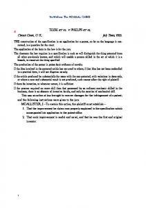
Outgroups_Pipidae_Rhinophrynus_dorsalis Outgroups_Pipidae_Xenopus_laevis Outgroups_Scaphiopodidae_Spea_bombifrons Outgroups_Scaphiopodidae_Scaphiopus_couchii Outgroups_Pelodytidae_Pelodytes_punctatus Outgroups_Pelobatidae_Pelobates_cultripes Outgroups_Megophryidae_Leptobrachium_boringii Outgroups_Megophryidae_Megophrys_nasuta Outgroups_Calyptocephalellidae_Calyptocephallela_gayi Outgroups_Calyptocephalellidae_Telmatobufo_venustus Outgroups_Myobatrachidae_Crinia_signifera Outgroups_Myobatrachidae_Limnodynastes_salmini Outgroups_Myobatrachidae_Lechriodus_melanopyga Outgroups_Myobatrachidae_Notaden_melanoscaphus Dendrobatidae_Allobates_femoralis Dendrobatidae_Anomaloglossus_verbeeksnyderorum Dendrobatidae_Rheobates_palmatus Dendrobatidae_Aromobates_saltuensis Dendrobatidae_Mannophryne_trinitatis Dendrobatidae_Hyloxalus_nexipus Dendrobatidae_Silverstoneia_nubicola Dendrobatidae_Epipedobates_tricolor Dendrobatidae_Ameerega_hahneli Dendrobatidae_Colostethus_pratti Dendrobatidae_Phyllobates_terribilis Dendrobatidae_Excidobates_captivus Dendrobatidae_Ranitomeya_ventrimaculata Dendrobatidae_Andinobates_claudiae Dendrobatidae_Minyobates_steyermarki Dendrobatidae_Adelphobates_galactonotus Dendrobatidae_Oophaga_histrionica Dendrobatidae_Dendrobates_auratus Hemiphractidae_Cryptobatrachus_sp_TNHCGDC451 Hemiphractidae_Flectonotus_fitzgeraldi Hemiphractidae_Gastrotheca_pseustes Hemiphractidae_Stefania_ginesi Hemiphractidae_Fritziana_ohausi Hemiphractidae_Hemiphractus_bubalus Ceuthomantidae_Ceuthomantis_smaragdinus Brachycephalidae_Ischnocnema_guentheri Brachycephalidae_Brachycephalus_ephippium Eleutherodactylidae_Phyzelaphryne_miriamae Eleutherodactylidae_Adelophryne_gutturosa Eleutherodactylidae_Eleutherodactylus_coqui Eleutherodactylidae_Diasporus_diastema Craugastoridae_Yunganastes_mercedesae Craugastoridae_Pristimantis_cruentus Craugastoridae_Lynchius_flavomaculatus Craugastoridae_Phrynopus_bracki Craugastoridae_Oreobates_quixensis Craugastoridae_Hypodactylus_brunneus Craugastoridae_Strabomantis_biporcatus Craugastoridae_Craugastor_podiciferus Craugastoridae_Haddadus_binotatus Craugastoridae_Bryophryne_cophites Craugastoridae_Barycholos_ternetzi Craugastoridae_Noblella_lochites Craugastoridae_Psychrophrynella_wettsteini Craugastoridae_Euparkerella_brasiliensis Craugastoridae_Holoaden_bradei Pelodryadinae_Nyctimystes_pulcher Pelodryadinae_Cyclorana_australis Pelodryadinae_Litoria_caerulea Phyllomedusinae_Cruziohyla_calcarifer Phyllomedusinae_Phasmahyla_cochranae Phyllomedusinae_Phyllomedusa_tomopterna Phyllomedusinae_Phrynomedusa_marginata Phyllomedusinae_Hylomantis_lemur Phyllomedusinae_Agalychnis_callidryas Phyllomedusinae_Pachymedusa_dacnicolor Hylinae_Scinax_staufferi Hylinae_Myersiohyla_kanaima Hylinae_Hyloscirtus_colymba Hylinae_Hypsiboas_raniceps Hylinae_Bokermannohyla_circumdata Hylinae_Aplastodiscus_perviridis Hylinae_Sphaenorhynchus_lacteus Hylinae_Xenohyla_truncata Hylinae_Dendropsophus_nanus Hylinae_Scarthyla_goinorum Hylinae_Pseudis_paradoxa Hylinae_Lysapsus_caraya Hylinae_Trachycephalus_venulosus Hylinae_Corythomantis_greeningi Hylinae_Aparasphenodon_brunoi Hylinae_Nyctimantis_rugiceps Hylinae_Argenteohyla_siemersi Hylinae_Itapotihyla_langsdorffii Hylinae_Tepuihyla_rodriguezi Hylinae_Osteocephalus_taurinus Hylinae_Phyllodytes_luteolus Hylinae_Osteopilus_septentrionalis Hylinae_Acris_crepitans Hylinae_Pseudacris_crucifer Hylinae_Plectrohyla_cyclada Hylinae_Exerodonta_chimalapa Hylinae_Ecnomiohyla_miliaria Hylinae_Ptychohyla_spinipollex Hylinae_Bromeliohyla_bromeliacia Hylinae_Duellmanohyla_rufioculis Hylinae_Charadrahyla_nephila Hylinae_Megastomatohyla_mixe Hylinae_Hyla_meridionalis Hylinae_Tlalocohyla_smithii Hylinae_Isthmohyla_pseudopuma Hylinae_Smilisca_phaeota Hylinae_Triprion_petasatus Hylinae_Anotheca_spinosa Ceratophryidae_Ceratophrys_cornuta Ceratophryidae_Lepidobatrachus_laevis Ceratophryidae_Chacophrys_pierottii Rhinodermatidae_Insuetophrynus_acarpicus Rhinodermatidae_Rhinoderma_darwinii Cycloramphidae_Zachaenus_parvulus Cycloramphidae_Cycloramphus_boraceiensis Cycloramphidae_Thoropa_miliaris Odontophrynidae_Proceratophrys_boiei Odontophrynidae_Macrogenioglottus_alipioi Odontophrynidae_Odontophrynus_occidentalis Telmatobiidae_Telmatobius_bolivianus Hylodidae_Crossodactylus_schmidti Hylodidae_Hylodes_nasus Hylodidae_Megaelosia_goeldii Batrachylidae_Atelognathus_patagonicus Batrachylidae_Batrachyla_leptopus Alsodidae_Limnomedusa_macroglossa Alsodidae_Alsodes_gargola Alsodidae_Eupsophus_calcaratus Leptodactylidae_Leptodactylus_melanonotus Leptodactylidae_Hydrolaetare_caparu Leptodactylidae_Lithodytes_lineatus Leptodactylidae_Adenomera_andreae Leptodactylidae_Rupirana_cardosoi Leptodactylidae_Scythrophrys_sawayae Leptodactylidae_Paratelmatobius_mantiqueira Leptodactylidae_Crossodactylodes_sp_MTR16370 Leptodactylidae_Pseudopaludicola_falcipes Leptodactylidae_Pleurodema_thaul Leptodactylidae_Edalorhina_perezi Leptodactylidae_Eupemphix_nattereri Leptodactylidae_Physalaemus_cuvieri Leptodactylidae_Engystomops_pustulosus Allophrynidae_Allophryne_ruthveni Centrolenidae_Hyalinobatrachium_fleischmanni Centrolenidae_Celsiella_revocata Centrolenidae_Ikakogi_tayrona Centrolenidae_Nymphargus_grandisonae Centrolenidae_Centrolene_savagei Centrolenidae_Teratohyla_spinosa Centrolenidae_Vitreorana_castroviejoi Centrolenidae_Chimerella_mariaelenae Centrolenidae_Espadarana_prosoblepon Centrolenidae_Cochranella_granulosa Centrolenidae_Rulyrana_adiazeta Centrolenidae_Sachatamia_albomaculata Bufonidae_Melanophryniscus_stelzneri Bufonidae_Frostius_erythrophthalmus Bufonidae_Atelopus_barbotini Bufonidae_Osornophryne_guacamayo Bufonidae_Oreophrynella_sp_ROM39649 Bufonidae_Amazophrynella_minuta Bufonidae_Dendrophryniscus_brevipollicatus Bufonidae_Nannophryne_variegata Bufonidae_Peltophryne_gundlachi Bufonidae_Rhaebo_haematiticus Bufonidae_Anaxyrus_americanus Bufonidae_Incilius_nebulifer Bufonidae_Rhinella_margaritifera Bufonidae_Nectophryne_afra Bufonidae_Bufo_gargarizans Bufonidae_Vandijkophrynus_robinsoni Bufonidae_Ansonia_longidigita


Figure A1: Backbone tree topology and posterior probabilities of clades from BEAST.

13

Appendix A from C. R. Hutter et al., Rapid Diversification and Time Explain Amphibian Richness at Different Scales in the Tropical Andes, Earth’s Most Biodiverse Hotspot Outgroups_Pipidae_Rhinophrynus_dorsalis Outgroups_Pipidae_Xenopus_laevis Outgroups_Scaphiopodidae_Spea_bombifrons Outgroups_Scaphiopodidae_Scaphiopus_couchii Outgroups_Pelodytidae_Pelodytes_punctatus Outgroups_Pelobatidae_Pelobates_cultripes Outgroups_Megophryidae_Leptobrachium_boringii Outgroups_Megophryidae_Megophrys_nasuta Outgroups_Calyptocephalellidae_Calyptocephallela_gayi Outgroups_Calyptocephalellidae_Telmatobufo_venustus Outgroups_Myobatrachidae_Crinia_signifera Outgroups_Myobatrachidae_Limnodynastes_salmini Outgroups_Myobatrachidae_Lechriodus_melanopyga Outgroups_Myobatrachidae_Notaden_melanoscaphus Dendrobatidae_Allobates_femoralis Dendrobatidae_Anomaloglossus_verbeeksnyderorum Dendrobatidae_Rheobates_palmatus Dendrobatidae_Aromobates_saltuensis Dendrobatidae_Mannophryne_trinitatis Dendrobatidae_Hyloxalus_nexipus Dendrobatidae_Silverstoneia_nubicola Dendrobatidae_Epipedobates_tricolor Dendrobatidae_Ameerega_hahneli Dendrobatidae_Colostethus_pratti Dendrobatidae_Phyllobates_terribilis Dendrobatidae_Excidobates_captivus Dendrobatidae_Ranitomeya_ventrimaculata Dendrobatidae_Andinobates_claudiae Dendrobatidae_Minyobates_steyermarki Dendrobatidae_Adelphobates_galactonotus Dendrobatidae_Oophaga_histrionica Dendrobatidae_Dendrobates_auratus Hemiphractidae_Cryptobatrachus_sp_TNHCGDC451 Hemiphractidae_Flectonotus_fitzgeraldi Hemiphractidae_Gastrotheca_pseustes Hemiphractidae_Stefania_ginesi Hemiphractidae_Fritziana_ohausi Hemiphractidae_Hemiphractus_bubalus Ceuthomantidae_Ceuthomantis_smaragdinus Brachycephalidae_Ischnocnema_guentheri Brachycephalidae_Brachycephalus_ephippium Eleutherodactylidae_Phyzelaphryne_miriamae Eleutherodactylidae_Adelophryne_gutturosa Eleutherodactylidae_Eleutherodactylus_coqui Eleutherodactylidae_Diasporus_diastema Craugastoridae_Yunganastes_mercedesae Craugastoridae_Pristimantis_cruentus Craugastoridae_Lynchius_flavomaculatus Craugastoridae_Phrynopus_bracki Craugastoridae_Oreobates_quixensis Craugastoridae_Hypodactylus_brunneus Craugastoridae_Strabomantis_biporcatus Craugastoridae_Craugastor_podiciferus Craugastoridae_Haddadus_binotatus Craugastoridae_Bryophryne_cophites Craugastoridae_Barycholos_ternetzi Craugastoridae_Noblella_lochites Craugastoridae_Psychrophrynella_wettsteini Craugastoridae_Euparkerella_brasiliensis Craugastoridae_Holoaden_bradei Pelodryadinae_Nyctimystes_pulcher Pelodryadinae_Cyclorana_australis Pelodryadinae_Litoria_caerulea Phyllomedusinae_Cruziohyla_calcarifer Phyllomedusinae_Phasmahyla_cochranae Phyllomedusinae_Phyllomedusa_tomopterna Phyllomedusinae_Phrynomedusa_marginata Phyllomedusinae_Hylomantis_lemur Phyllomedusinae_Agalychnis_callidryas Phyllomedusinae_Pachymedusa_dacnicolor Hylinae_Scinax_staufferi Hylinae_Myersiohyla_kanaima Hylinae_Hyloscirtus_colymba Hylinae_Hypsiboas_raniceps Hylinae_Bokermannohyla_circumdata Hylinae_Aplastodiscus_perviridis Hylinae_Sphaenorhynchus_lacteus Hylinae_Xenohyla_truncata Hylinae_Dendropsophus_nanus Hylinae_Scarthyla_goinorum Hylinae_Pseudis_paradoxa Hylinae_Lysapsus_caraya Hylinae_Trachycephalus_venulosus Hylinae_Corythomantis_greeningi Hylinae_Aparasphenodon_brunoi Hylinae_Nyctimantis_rugiceps Hylinae_Argenteohyla_siemersi Hylinae_Itapotihyla_langsdorffii Hylinae_Tepuihyla_rodriguezi Hylinae_Osteocephalus_taurinus Hylinae_Phyllodytes_luteolus Hylinae_Osteopilus_septentrionalis Hylinae_Acris_crepitans Hylinae_Pseudacris_crucifer Hylinae_Plectrohyla_cyclada Hylinae_Exerodonta_chimalapa Hylinae_Ecnomiohyla_miliaria Hylinae_Ptychohyla_spinipollex Hylinae_Bromeliohyla_bromeliacia Hylinae_Duellmanohyla_rufioculis Hylinae_Charadrahyla_nephila Hylinae_Megastomatohyla_mixe Hylinae_Hyla_meridionalis Hylinae_Tlalocohyla_smithii Hylinae_Isthmohyla_pseudopuma Hylinae_Smilisca_phaeota Hylinae_Triprion_petasatus Hylinae_Anotheca_spinosa Ceratophryidae_Ceratophrys_cornuta Ceratophryidae_Lepidobatrachus_laevis Ceratophryidae_Chacophrys_pierottii Rhinodermatidae_Insuetophrynus_acarpicus Rhinodermatidae_Rhinoderma_darwinii Cycloramphidae_Zachaenus_parvulus Cycloramphidae_Cycloramphus_boraceiensis Cycloramphidae_Thoropa_miliaris Odontophrynidae_Proceratophrys_boiei Odontophrynidae_Macrogenioglottus_alipioi Odontophrynidae_Odontophrynus_occidentalis Telmatobiidae_Telmatobius_bolivianus Hylodidae_Crossodactylus_schmidti Hylodidae_Hylodes_nasus Hylodidae_Megaelosia_goeldii Batrachylidae_Atelognathus_patagonicus Batrachylidae_Batrachyla_leptopus Alsodidae_Limnomedusa_macroglossa Alsodidae_Alsodes_gargola Alsodidae_Eupsophus_calcaratus Leptodactylidae_Leptodactylus_melanonotus Leptodactylidae_Hydrolaetare_caparu Leptodactylidae_Lithodytes_lineatus Leptodactylidae_Adenomera_andreae Leptodactylidae_Rupirana_cardosoi Leptodactylidae_Scythrophrys_sawayae Leptodactylidae_Paratelmatobius_mantiqueira Leptodactylidae_Crossodactylodes_sp_MTR16370 Leptodactylidae_Pseudopaludicola_falcipes Leptodactylidae_Pleurodema_thaul Leptodactylidae_Edalorhina_perezi Leptodactylidae_Eupemphix_nattereri Leptodactylidae_Physalaemus_cuvieri Leptodactylidae_Engystomops_pustulosus Allophrynidae_Allophryne_ruthveni Centrolenidae_Hyalinobatrachium_fleischmanni Centrolenidae_Celsiella_revocata Centrolenidae_Ikakogi_tayrona Centrolenidae_Nymphargus_grandisonae Centrolenidae_Centrolene_savagei Centrolenidae_Teratohyla_spinosa Centrolenidae_Vitreorana_castroviejoi Centrolenidae_Chimerella_mariaelenae Centrolenidae_Espadarana_prosoblepon Centrolenidae_Cochranella_granulosa Centrolenidae_Rulyrana_adiazeta Centrolenidae_Sachatamia_albomaculata Bufonidae_Melanophryniscus_stelzneri Bufonidae_Frostius_erythrophthalmus Bufonidae_Atelopus_barbotini Bufonidae_Osornophryne_guacamayo Bufonidae_Oreophrynella_sp_ROM39649 Bufonidae_Amazophrynella_minuta Bufonidae_Dendrophryniscus_brevipollicatus Bufonidae_Nannophryne_variegata Bufonidae_Peltophryne_gundlachi Bufonidae_Rhaebo_haematiticus Bufonidae_Anaxyrus_americanus Bufonidae_Incilius_nebulifer Bufonidae_Rhinella_margaritifera Bufonidae_Nectophryne_afra Bufonidae_Bufo_gargarizans Bufonidae_Vandijkophrynus_robinsoni Bufonidae_Ansonia_longidigita

20.0

14


Figure A2: Confidence intervals on dates for the backbone tree from BEAST. Tree files with divergence dates (median ages) are available on the Dryad Digital Repository: http://dx.doi.org/10.5061/dryad.1555n (Hutter et al. 2017).

15


Appendix B from C. R. Hutter et al., “Rapid Diversification and Time Explain Amphibian Richness at Different Scales in the Tropical Andes, Earth’s Most Biodiverse Hotspot” (Am. Nat., vol. 190, no. 6, p. 000) Detailed Species Richness Methods and Results Methods We compiled species geographic distributions and elevational ranges from the Global Amphibian Assessment (GAA; IUCN 2014) to quantify richness for (1) seven major biogeographic regions across South America and (2) elevational zones in the Tropical Andes and adjacent lowlands. We collected data for species not present in the GAA from species descriptions (frequently updated species lists for each family taken from AmphibiaWeb 2016). To analyze patterns of elevational richness within clades, we selected 10 strongly supported groups. Strongly supported clades were identified from our own analyses and following Pyron and Wiens (2011). These 10 clades consisted mostly of families and subfamilies but also included a group of families (the Austral clade described above). We chose clades that were distributed in the Andes or South American lowlands and excluded those occurring predominantly in non-Andean highland regions (e.g., high elevations of the Atlantic Forest region and the tepuis of the Guiana Shield). These 10 clades collectively include 91% of South American hyloid species. When calculating Andean and lowland richness patterns, we did not include occurrences of species in these other highland regions that were above 799 m, since they were not relevant for Andean (or lowland) richness patterns. All data aggregation, manipulation, and summarization were completed in the statistical software package R, version 3.1 (R Core Team 2016). For the regional-scale analyses, seven biogeographic regions were used. These generally followed Duellman (1999), who identified regions based on patterns of frog endemism. The regions used were Amazonia, Tropical Andes (combined North and Central Andes), Atlantic Forest, Choco, Cerrado (including the combined Cerrado, Caatinga, and Choco regions), Guiana Shield, and temperate South America (fig. 1). We differed from Duellman (1999) in that we combined the North and Central Andes because we aimed to address species richness patterns of the Tropical Andes relative to other regions and not individual subdivisions of the Andes. We considered the southern Andes to be part of temperate South America. Finally, we created vectorized shapefiles for each selected region by using the Terrestrial Ecoregions of the World resource from the World Wildlife Fund (Olson et al. 2001). To determine each species’ regional occurrence, we used species’ distribution maps from the GAA (as minimum convex polygons) and the R package raster (Hijmans 2012) to calculate each species’ percent occurrence in each region. We ensured that the elevational distributions of species (from GAA) were consistent with these regional categorizations (e.g., no species occurring in low-elevation regions with a high-montane elevational range). A potential concern is that the regions could have uncertain borders due to spatial uncertainty. Therefore, we manually examined species that occurred near region borders as well as species that occurred across multiple regions with a polygon overlap less than 50% to ensure that the species actually occurred in that region (using the GAA species accounts and locality information). Additionally, we considered species as occurring in a biogeographic region if the region included 110% of the species’ range (otherwise minimum convex polygons sometimes overlapped a region that a species was not known to occur in). Species that did not have range maps typically were newly described species, so we consulted the original descriptions for biogeographic data. We did not use species distribution modeling (SDM, such as with MaxEnt) to predict the presence of a species in a given region, as many species are known from too few localities and are regional endemics. Furthermore, use of SDM could result in overpredicting species ranges into regions where they do not actually occur and overestimation of regional richness. Indeed, SDMs are known to generally overpredict species ranges in amphibians, especially in the Neotropics (Munguía et al. 2012). Therefore, we used known species ranges rather than predicted species ranges. We then summed the number of species occurring in each biogeographic region. We defined species occurring from 0 to 900 m as lowland, those between 800 and 6,000 m as Andean, and those !800 m and 1900 m as both (recall that non-Andean highland species were excluded; see above). These limits were based on the average lower limit of Andean montane forests (Hooghiemstra et al. 2006; Hoorn et al. 2010). The 100-m overlap was added to prevent coding species as both due to extremes in their distributions. Based on our data, no species are 1

Appendix B from C. R. Hutter et al., Rapid Diversification and Time Explain Amphibian Richness at Different Scales in the Tropical Andes, Earth’s Most Biodiverse Hotspot

distributed exclusively between 800 and 900 m. We found that the South American lowlands (!900 m) contain 1,583 species (i.e., across all six non-Andean regions). The Tropical Andes have 1,260 species (figs. 1, 3A). To assess elevational richness patterns, we first placed each species in one or more elevational bands based on the lower and upper limits of its elevational distributions for the Tropical Andes. We considered only hyloids distributed in the Tropical Andes and excluded the highland distributions of species from other South American highland regions (Guiana Shield, Atlantic Forest, temperate Andes). We used 500-m bands from 0 to 6,000 m (e.g., 0–500, 501–1,000), following standard practice (Rahbek 1997; Kozak and Wiens 2010b; Hutter et al. 2013). One past study has shown that reducing the bin size (e.g., 200-m bins) improved the fit of statistical relationships (Hutter et al. 2013). However, this presumably occurred because of pseudoreplication of the existing richness from the 500-m bins. Species with range extremes ending on the limits of a band were not counted for the adjacent band (a range of 500–1,001 would only count for 501–1,000, not 0–1,500). We then summed the species present in each band to estimate the richness of the band.

2


Appendix C from C. R. Hutter et al., “Rapid Diversification and Time Explain Amphibian Richness at Different Scales in the Tropical Andes, Earth’s Most Biodiverse Hotspot” (Am. Nat., vol. 190, no. 6, p. 000) BAMM Analysis: Detailed Methods and Results Methods We assessed diversification rates and evolution of elevational distributions using the Bayesian analysis of macroevolutionary mixtures program (BAMM 2.5, Nov. 2015; Rabosky 2014). BAMM uses reversible-jump Markov chain Monte Carlo to sample models with differing numbers and types of rate regimes, which are branches of the tree that share the same rate of diversification or trait evolution. Additionally, BAMM can identify areas of the tree with strong support for a regime shift (significant increases or decreases in rates). BAMM incorporates varying rates through time (while switching between time-constant and time-varying functions, when supported by the underlying data) through an exponential change function (Rabosky 2014). We used BAMM to test two hypotheses: (1) the diversification rate hypothesis, which would be supported when diversification rates are positively related to species richness in different major biogeographic regions or different Andean elevational zones; and (2) the hypothesis that changing elevational distributions (and related shifts in climatic distributions) drive speciation, which would be supported if diversification rates are positively related to rates of change in elevational distributions. Additionally, extinction rates might be decoupled from speciation rates; however, we do not consider this problematic for our analysis, as speciation rates are strongly correlated with diversification rates for species (Spearman’s rank correlation: rs p 0:701; P ! :001; n p 2,318). First, we used the R package BAMMtools (ver. 2.1.0; Rabosky et al. 2014; R Core Team 2016) and the full hyloid phylogeny of 2,318 species to estimate appropriate priors for each analysis (see table C1 for priors used). We note that we tested the effect of modifying the Poisson rate prior (1.0, 0.5, 0.1), where smaller values can increase the number of distinct diversification rate regimes on the phylogeny. We found that all three Poisson rate priors (PRP) tested gave similar results and that all of our significant shifts were detected using the most conservative prior (PRP p 1:0; results not shown). For both analyses, we also constrained shifts to occur only for clades with 25 species or more, as numerous shifts might be supported within a genus. This is important because we are interested in patterns of diversification on larger scales, not within smaller groups of species. Results differed by only the number of shifts within genera (e.g., for Atelopus, we found three shifts with no constraints and one shift with the constraint; results not shown). For diversification analyses, we accounted for described but unsampled species (excluding counts from undescribed species sampled in the phylogeny) by estimating the fraction of species sampled from each genus for the diversification analyses. BAMM incorporates this fraction into parameter estimation using the method developed by FitzJohn et al. (2009). Simulations suggest that this method performs adequately if sampling is 150% (FitzJohn et al. 2009). Here we have included 64% of described species sampled for Hyloidea within South America. We ran an R script to determine optimal Metropolis coupled MCMC parameters to facilitate convergence, which were nine chains, a deltaT p 0:005, and 1,000 generations for each chain swap proposal (script available from https://github.com/macroevolution/ bamm). We ran each analysis twice for 500 million generations, sampling every 500,000 generations. Finally, we checked that each replicate run was consistent, based on a Spearman’s rank test on the rates estimated per species (the location and number of shifts was also checked for consistency). The samples from the two analyses were then combined (after discarding burn-in) upon consistent convergence and rate estimates. See the main text (fig. 1) for a phylorate plot of the rates on the phylogeny through time. For analyses of rates of elevational distribution, we coded each species based on its Andean elevational midpoint (midpoint p (maximum elevation 2 minimum elevation=2) 1 minimum elevation), after excluding non-Andean highland elevational distributions (see table S3). For the analyses of rates of trait evolution, incomplete taxon sampling is not corrected for in BAMM. However, this should not be problematic given the assumption that species were sampled randomly with respect to the trait in question (Rabosky 2014). Supporting the assumption of random sampling, the

1

Appendix C from C. R. Hutter et al., Rapid Diversification and Time Explain Amphibian Richness at Different Scales in the Tropical Andes, Earth’s Most Biodiverse Hotspot

elevational richness patterns of sampled species (i.e., number of species included in the tree in each 500-m band) were strongly correlated with those for all species (Spearman’s rank correlation: rs p 0:979; P ! :001). To estimate rates of elevational distribution, we ran each trait-based BAMM analysis twice for 1 billion generations each, sampling every 1 million generations. For these analyses, we used the default Metropolis-coupled MCMC parameters as the analyses rapidly converged (four chains, deltaT p 0:1, swap period p 1,000 generations). Finally, we checked that each replicate run was consistent based on significant support from a Spearman’s rank test on the individual rates per species between replicates (Spearman’s rank p rs p 0:978–0:995; P ! :001). The samples from the two analyses were then combined after finding consistent convergence and rate estimates. A phylorate plot with the rates and significant shifts is shown in figure 2. We used the R package coda (Plummer et al. 2016) with the BAMM output to assess MCMC convergence by evaluating whether the likelihood had reached stationarity. We discarded as burn-in the first 10% of the generations for diversification analyses and 25% for trait analyses. The likelihoods consistently reached stationarity by these two points in these two sets of analyses. We also confirmed that the effective sample size of the log likelihood and number of parameter shifts were greater than 200. Using BAMMtools, we estimated the overall best number of rate shifts by simulating a null model with no rate shifts and compared it to each model represented by a distinct number of shifts. We calculated a Bayes factor score for each model with a unique number of shifts relative to the null model, selecting the model with the highest score (Rabosky et al. 2014). Additionally, to determine the best rate-shift configuration on the tree, we calculated the 95% credible set of distinct shift configurations, which is the set of shift configurations that accounts for 95% of the probability distribution of the data. We considered only the number of shifts from the best model selected through Bayes factor scores and chose the configuration with the highest posterior probability (see fig. C1 for the 95% credible set of configurations). To test the relationship between diversification rates and elevational distributions of genera, we first calculated the midpoint elevation (see above) for each species’ elevational range and calculated the mean and median of these values across species for each genus. The mean and median of the elevational ranges of genera were significantly correlated (Spearman’s rank: rs p 0:955; P ! :001), so we used the mean, as results should not differ. We extracted the mean and median rate of evolution (from posterior rate distributions) for elevational distributions and diversification rates for species. The mean and median for each of the rate sets were significantly correlated (Spearman’s rank correlation: rs p 0:961–0:985; P ! :001), so again we used the mean. To test the relationships between elevational midpoint and diversification rates and between rate of evolution of elevational distributions, we used phylogenetic generalized least squares (PGLS) regression (Martins and Hansen 1997) in ape (ver. 3.0; Paradis et al. 2004). Prior to PGLS regression, we compared four models of continuous trait evolution for the mean elevation of genera and the rate of evolution for elevational distributions: (1) the white noise model, in which traits evolve independently of phylogeny; (2) the Brownian motion model, in which trait evolution follows a random walk and is perfectly correlated with the phylogeny; (3) the l model, in which a maximum likelihood estimate of Pagel’s (1999) l is used to estimate the degree that trait evolution is explained by phylogeny under a random walk model (where a l of 1 is equivalent to the Brownian motion model and 0 is equivalent to white noise); and (4) Ornstein-Uhlenbeck (OU), a constrained random walk where traits tend to deviate from a single optimal value but also tend to return to this optimum at a given estimated rate. We then calculated the sample-size-corrected Akaike information criterion (AICc) to compare the log-likelihood values of these models (while accounting for the different numbers of parameters) and selected the best model as that with the lowest AICc (Burnham and Anderson 1998). Finally, we used PGLS regression with the R package ape after transforming the tree to the best-fit model of trait evolution (and associated parameter estimates) to test our hypotheses across hyloid phylogeny and within each selected family/ subfamily clade. A potential concern with using rates derived from BAMM is that these rates can be significantly autocorrelated due to shared rate regimes among species (see similarity in rates among related species in fig. 2). Therefore, PGLS regression might overestimate the correlation error structure of the BAMM-extracted rate data (Rabosky et al. 2013). To address this, we used a permutation test on the F statistic from PGLS regression to generate a null distribution of test-statistic values derived from shuffling the rate of evolution of elevational distributions among genera on the full phylogeny using R. We tested each data set for the best model of evolution (see above) and used PGLS regression and collected each F statistic. We ran this analysis for 1,000 repetitions. Finally, we compared the observed F statistics calculated from the full and subset data sets to the null distribution of F and calculated a P value by finding the percentage of F values from the null distribution that are greater than the observed F. 2


We used an alternative approach to test the diversification rate hypothesis by estimating diversification rates and species richness for biogeographic regions and elevational zones directly. We used the species richness and diversification rates for species that were estimated above, calculating the mean rate across all species that occur in each region or elevational zone. We then used standard linear regression to test the hypothesis that rates are related to species richness of elevational zones or regions, where a positive relationship would support the diversification rate hypothesis. This approach is advantageous in more directly testing the hypothesis that rates and richness patterns are related, relative to testing for a relationship between rates and elevational midpoints. We created the phylorate plot (fig. 2) by using BAMMtools to map the diversification rates and significant shifts on the chronogram (Rabosky et al. 2014). We used the Jenks break method (rates are binned to minimize within-bin variance and maximize among-bin variance) to partition rates into a temperature-based color scheme. The elevational distribution plot was created from the ancestral reconstructions of elevational midpoints (described in “Supplemental Appendix”; data deposited in the Dryad Digital Repository: http://dx.doi.org/10.5061/dryad.1555n [Hutter et al. 2017]) by binning the elevations into a temperature-based color scheme and mapping them to the chronogram using the R package phytools (Revell 2012). When compared to similar methods (e.g., clade based, state-dependent speciation and extinction [SSE] models, medusa), BAMM provides advantages by explicitly incorporating diversity dependence, variable rates through time within regimes, limited reliance on clade delimitation, and a simple visualization of how diversification rates change across the phylogeny. However, some authors have shown that this method can perform poorly in simulations (Moore et al. 2016). Therefore, we also used clade and SSE-based analyses to address whether these results were consistent with the BAMM results.

Results The results for the hypotheses tested above are included in the main text. Significant shifts in diversification rate are visually displayed in figure 2, and details for each shift and the clades they correspond with are shown in table C2. The credible shift and their marginal probabilities were also examined and are included in figure C1. Significant shifts in the rate of evolution of elevations are visually displayed in figure C2. The results for the diversification rate hypothesis for each family-level clade are included in table C2, while the results that test for relationships between diversification rates and elevational rates of change among genera within families are included in table C4. The rates calculated for each genus are included in table C5.

Tables and Figures Table C1: Priors estimated from BAMMtools for each analysis type Parameter

Diversification prior

Trait prior

Lambda/Beta InitPrior Lambda/Beta ShiftPrior muInitPrior IsTimeVariablePrior

2.88604905841161 .0113263663307018 2.88604905841161 1 (yes)

9.09148740270706e-06 .0113263663307018 ... 1 (yes)

Note: The diversification rate analyses priors are for the lambda (speciation) parameter, whereas the trait analyses estimate the beta (rate of change in traits) parameter. The priors were also used as the initial parameter values. Parameters are defined as follows: InitPrior p prior on the diversification/trait rate; ShiftPrior p prior on the number of diversification/trait rate shifts; muInitPrior p prior on the extinction rate; IsTimeVariablePrior p enabling rates to vary through time by coding as 1; Lambda p speciation rate; mu p extinction rate; and Beta p trait evolution rate.

3


Table C2: Significant increases in speciation rates detected by Bayesian analysis of macroevolutionary mixtures (BAMM) Clade

Majority region

Midpoint elevation (m)

No. species

Age (Ma)

Speciation (95% CI)

Terrarana 1 Hemiphractidae Pristimantis (Pristimantinae) Centrolenidae Eleutherodactylidae Gastrotheca (Hemipractidae) Rhinella (Bufonidae) Atelopus (Bufonidae) Telmatobiidae

Tropical Andes Tropical Andes Tropical Andes West Indies Tropical Andes Atlantic Forest Tropical Andes Tropical Andes

1,610 1,800 1,255 ... 2,620 500 3,175 3,550

680 239 128 95 41 71 31 60

93.0 46.9 33.4 38.1 33.0 27.4 13.3 21.9

.065 (.064–.065) .091 (.09–.093) .114 (.112–.115) .075 (.073–.077) .091 (.086–.096) .223 (.215–.23) .469 (.443–.495) .693 (.663–.723)

Diversification (95% CI) .057 .078 .103 .068 .072 .128 .164 .516

(.056–.057) (.077–.079) (.101–.105) (.066–.07) (.069–.075) (.123–.134) (.15–.177) (.491–.541)

Note: Eight significant speciation rate increases were detected, which were each supported by significantly higher Bayes factor scores. Five shifts occurred within clades distributed primarily in the Tropical Andes. The majority region is the region where the majority of the species in the clade occur. The midpoint elevation, number of species, and age are calculated for the species following a rate shift. The speciation and diversification rates are estimated from the BAMM output for the node closest to the shift. The confidence intervals (CI) are calculated from a normal distribution of rate values derived from the posterior distribution of rate estimates. We note that BAMM estimates only significant shifts in speciation rates; however, the diversification rate is strongly correlated with the speciation rate, so the shifts can also represent significant increases in diversification rate.

Table C3: Diversification rate hypothesis results for each tested clade Test statistics Clade Aromobatinae (Dendrobatidae) Bufonidae Centrolenidae Dendrobatinae (Dendrobatidae) Hemiphractidae Hylinae (Hylidae) Leptodactylidae Pristimantinae (Craugastoridae) Phyllomedusinae (Hylidae) Telmatobiidae

Richness peak

R2

P

Lowland Lowland 1 Andes Andes Lowlands Andes Lowlands Lowlands Andes Lowlands Andes

.394 .008 .037 .145 .689 .012 .118 .064 .011 .047

.554 .857 .736 .221 .043 .712 .925 .714 .917 .761

Note: A relationship between diversification rates estimated from BAMM and richness of each 500-m band in the Andes was tested. Boldface indicates significance.

Table C4: Results from analyses of the relationship between ln-transformed diversification rates and lntransformed rates of change in elevational distributions (i.e., trait rate from BAMM) using phylogenetic generalized least squares regression Test statistics Clade Aromobatinae (Dendrobatidae) Bufonidae Centrolenidae Dendrobatinae (Dendrobatidae) Hemiphractidae Hylinae (Hylidae) Leptodactylidae Pristimantinae (Craugastoridae) Phyllomedusinae (Hylidae)

2

Richness peak

No. genera

R

P

Lowland Lowland 1 Andes Andes Lowlands Andes Lowlands Lowlands Andes Lowlands

5 13 12 13 6 23 14 5 6

.487 .036 .514 .001 .132 .040 .003 .984 .432

.190 .624 .035 .907 .479 .474 .860 .008 .579

Note: Rates were derived from BAMM and estimated for genera within each family-level clade. Telmatobiidae was excluded from this analysis as it has only one genus. Boldface indicates significance.

4


Table C5: Data for genera used in testing the diversification rate hypothesis and for testing whether there is a relationship between diversification rates (species/myr) and rates of change in elevational distributions (i.e., trait rate) Elevations Clade Adelophryne Adelphobates Adenomera Agalychnis Allobates Allophryne Alsodes Amazophrynella Ameerega Andinobates Anomaloglossus Aplastodiscus Aromobates Atelognathus Atelopus Bokermannohyla Brachycephalus Bryophryne Celsiella Centrolene Ceratophrys Chacophrys Chimerella Cochranella Colostethus Craugastor Crossodactylodes Cruziohyla Cryptobatrachus Cycloramphus Dendrobates Dendrophryniscus Dendropsophus Diasporus Edalorhina Engystomops Epipedobates Espadarana Euparkerella Eupsophus Excidobates Flectonotus Fritziana Frostius Gastrotheca Haddadus Hemiphractus Hyalinobatrachium Hydrolaetare Hylodes Hyloscirtus Hyloxalus Hypodactylus Hypsiboas Ikakogi Ischnocnema Leptodactylus

Sampled (total) 9 4 41 5 58 1 18 6 28 8 18 7 10 5 31 5 4 1 2 24 5 1 2 9 3 3 5 1 3 5 4 5 74 1 1 14 8 7 5 15 3 2 5 1 56 1 5 31 1 7 19 36 5 59 1 27 54

(12) (4) (41) (9) (76) (3) (21) (6) (35) (12) (28) (10) (19) (12) (99) (12) (6) (6) (2) (34) (12) (1) (2) (16) (18) (4) (5) (3) (8) (20) (5) (5) (117) (4) (2) (14) (10) (8) (5) (15) (3) (2) (5) (2) (70) (1) (6) (34) (2) (24) (32) (72) (13) (79) (1) (30) (77)

Diversification rate

Trait rate (m)

Lower

Upper

Mean

.059 .541 .039 .061 .189 .064 .060 .065 .061 .090 .185 .032 .140 .060 .071 .079 .059 .064 .076 .040 .059 .064 .040 .036 .063 .060 .041 .064 .058 .059 .516 .043 .059 .064 .064 .038 .057 .040 .062 .060 .168 .058 .058 .064 .058 .064 .058 .072 .064 .059 .034 .541 .059 .075 .064 .058 .039

15,843.8 16,025.8 11,971.8 9,275.5 7,837.5 25,262.8 175,243.4 34,587.5 16,380.8 16,289.2 24,732.6 15,751.3 16,387.7 34,609.7 150,015.7 15,711.8 25,907.2 25,262.8 35,540.4 37,440.3 10,685.3 25,262.8 35,506.2 35,741.5 16,140.1 15,629.3 9,219.5 25,262.8 15,673.3 34,447.1 16,136.6 34,839.5 37,103.8 25,262.8 25,262.8 23,590.7 16,545.4 35,797.2 16,217.7 84,032.8 16,705.8 15,427.2 15,859.6 25,262.8 16,095.9 25,262.8 15,608.5 35,789.6 25,262.8 34,069.8 15,668.8 16,351.0 15766.9 27,518.6 25,262.8 15,904.8 9,243.5

418 150 241 426 336 74 778 164 459 1,225 353 253 1,880 667 1,822 358 522 3,142 975 1,732 265 70 803 417 1,108 0 408 83 1,099 245 70 334 422 175 160 240 541 851 151 182 926 550 479 70 1,852 0 392 602 79 377 1,723 1,228 2,303 335 980 435 127

658 350 444 842 544 242 1,450 500 899 1,573 670 677 2,411 1,086 2,407 660 668 3,534 1,799 2,271 584 200 1,165 1,030 1,543 1,315 651 500 1,748 581 582 599 877 995 1,050 831 1,166 1,539 475 934 1,037 1,300 700 799 2,487 799 1,685 1,151 209 679 2,451 1,696 2,757 900 1,790 737 878

650 100 316 380 300 150 1,051 275 537 1,740 437 492 2,345 825 2,391 505 725 3,357 1,387 1,950 225 135 984 598 1,375 675 600 325 1,450 400 300 472 400 595 605 475 812 1,215 300 525 1,001 925 650 435 2,378 400 1,150 758 144 612 2,279 1,436 2,900 500 1,385 650 400

5


Table C5 (Continued ) Elevations Clade Lithodytes Lynchius Mannophryne Melanophryniscus Nannophryne Noblella Nymphargus Odontophrynus Oophaga Oreobates Osornophryne Osteocephalus Paratelmatobius Phasmahyla Phrynopus Phyllobates Phyllodytes Phyllomedusa Physalaemus Phyzelaphryne Pleurodema Pristimantis Proceratophrys Pseudis Pseudopaludicola Psychrophrynella Ranitomeya Rhaebo Rheobates Rhinella Rhinoderma Rulyrana Sachatamia Scarthyla Scinax Silverstoneia Smilisca Sphaenorhynchus Stefania Strabomantis Telmatobius Tepuihyla Teratohyla Trachycephalus Vitreorana Xenohyla Yunganastes

Sampled (total) 1 4 17 7 2 4 21 4 3 22 11 26 2 3 13 3 6 26 18 3 13 206 14 9 17 8 20 4 1 57 2 8 4 2 40 2 2 2 4 5 36 3 4 9 7 1 4

(1) (4) (23) (20) (4) (11) (41) (8) (4) (24) (12) (29) (3) (5) (24) (3) (16) (28) (43) (4) (13) (457) (22) (11) (21) (23) (23) (12) (2) (94) (3) (10) (4) (3) (93) (3) (2) (11) (7) (15) (74) (3) (4) (13) (7) (2) (4)

Diversification rate

Trait rate (m)

Lower

Upper

Mean

.064 .064 .128 .042 .035 .061 .067 .060 .541 .066 .066 .073 .033 .059 .059 .541 .063 .060 .067 .062 .068 .061 .059 .061 .062 .059 .057 .042 .064 .040 .059 .040 .043 .063 .078 .058 .093 .067 .058 .062 .061 .067 .049 .065 .034 .064 .059

25,262.8 15,984.5 16,410.3 37,905.2 38,373.8 15,880.2 35,802.0 10,579.2 16,051.7 16,205.8 39,162.6 30,265.2 10,841.4 9,530.2 16,095.9 15,746.5 9,307.9 9,456.3 9,083.1 15,603.2 99,693.7 40,678.6 9,814.4 9,405.0 17,173.1 15,868.1 16,347.9 39,181.7 25,262.8 39,832.8 33,011.9 35,832.8 35,666.1 9,172.1 9,459.8 16,392.2 8,918.7 9,541.6 16,045.3 15,769.9 51,595.0 160,247.0 35,573.6 9,392.4 35,596.7 25,262.8 16,847.6

0 2,389 572 173 1,994 1,576 1,577 543 225 1,138 2,571 393 587 338 3138 68 72 343 140 208 646 1,565 250 164 283 3,208 111 747 225 721 33 839 193 82 204 583 0 54 435 772 2,799 1,045 152 104 263 0 1,875

1,799 2,743 1,063 491 3,031 2,297 2,026 1,357 850 1,624 3,557 866 790 655 3,294 908 488 964 588 353 1,780 2,170 601 484 626 3,595 533 1,312 2,000 1,402 600 1,533 1,318 301 682 1,233 1,050 349 811 1,632 3,630 1,123 598 610 799 425 2,550

900 2,751 820 230 2,710 2,000 1,850 888 500 1,262 3,100 450 650 425 3,260 545 263 500 400 300 850 1,970 425 250 400 3,466 250 755 1,112 700 250 1,194 750 200 400 900 525 175 614 1,171 3,300 692 315 300 625 212 2,225

Note: Rates are estimated for each genus from BAMM using the mean rates of the species included in each genus.

6


f = 0.015

f = 0.015

f = 0.0076

f = 0.0076

f = 0.0076

f = 0.0076

f = 0.0076

f = 0.0076

f = 0.0076

Figure C1: Ninety-five percent Bayesian credible set of distinct shift configurations that account for 95% of the probability distribution of the data. The value shown is the proportion of samples in the posterior distribution that support that shift configuration. Proportions sum to 1; however, many weakly supported shift configurations are not shown.

7


Rate of evolution of elevational distributions

5,000

690,000

16,000

Dendrobatinae Aromobatinae

Phyllomedusinae

Hylinae

Leptodactylidae

Centrolenidae Bufonidae Telmatobiidae

Pristimantinae

Hemiphractidae

Figure C2: Rate of evolution of elevational distributions for Hyloidea from the BAMM results plotted on the phylogeny. The red circles indicate significant increases in rate.

8


Appendix D from C. R. Hutter et al., “Rapid Diversification and Time Explain Amphibian Richness at Different Scales in the Tropical Andes, Earth’s Most Biodiverse Hotspot” (Am. Nat., vol. 190, no. 6, p. 000) Alternative Diversification Analyses Methods To further test the diversification rate hypothesis for biogeographic regions and elevations in the Andes, we used two main alternative approaches, in addition to Bayesian analysis of macroevolutionary mixtures (BAMM; which is used in the main text). (1) We used a clade-based method (Magallón and Sanderson 2001) that incorporates all species, including those not sampled in the phylogeny. We used this approach to test the influence of both geographic regions and elevational zones on diversification rates by averaging the diversification rates of species from clades occurring in each region and zone (see below). (2) We assessed the influence of lowland versus Andean distribution (independent of clade delimitation) on diversification rates using the geographic speciation and extinction likelihood approach (GeoSSE; Goldberg et al. 2011). Given the hypothesis that changing elevational distributions (and related shifts in climatic distributions) may drive speciation (Moritz et al. 2000; Kozak and Wiens 2010a; Hua and Wiens 2013), we also tested whether there is a relationship between diversification rates and rates of change in elevation within clades, using clade-based methods. We used clade-based analyses for the estimation of rates of change in elevation and the diversification rates calculated via the first approach above (Magallon and Sanderson 2001).

Clade-Based Analyses To assess the robustness of our diversification results from BAMM, we assessed the relationship between species richness and diversification rates within regions and binned elevational zones using a clade-based alternative. Specifically, we estimated diversification rates of genera using the method-of-moments estimators (Magallón and Sanderson 2001) and then tested for relationships between these rates and (a) richness of large-scale biogeographic regions, (b) richness of elevational zones in the Andes, (c) the elevational distribution (i.e., elevational midpoints) of genera, and (d) rates of change in elevational distributions among species within genera. To calculate clade-based rates, we used the backbone tree and family trees (with genera within families as units). We estimated a diversification rate for each genus using the method-of-moments estimator for stem and crown group ages (Magallón and Sanderson 2001) in the R package geiger (ver. 2.0; Harmon et al. 2008; Pennell et al. 2014; R Core Team 2016). All genera were monophyletic. This method estimates diversification rates based on clade ages (stem or crown), species richness, and an assumed relative extinction fraction (ε). Clade ages were obtained from the phylogeny. Species richness for each genus (including all described species, not just those in the tree) was obtained from AmphibiaWeb (2016), but we also included those well-supported, undescribed species sampled in our tree. We used three standard values of ε (0, 0.45, 0.90; table D1). Each analysis applied a particular value of ε across all clades. Note that ε is intended to correct for the failure to sample clades entirely, is meant to be applied across the entire tree, and is not intended as an estimate of extinction rates in individual clades (Magallón and Sanderson 2001). Use of stem group ages should mitigate incomplete sampling in the phylogeny better than crown group ages, given that the inclusion of only a single species will capture the stem group age, whereas dozens of species may need to be sampled to be certain of the crown group age. Undersampling may lead to underestimating the crown age and overestimating diversification rates. Monotypic genera were left out of the crown group analyses, as these rates could not be calculated (because monotypic clades do not have a crown group age). The diversification rates estimated across these different ages and relative extinction rates are presented in table D1. Recent simulations show that this method can give accurate estimates of diversification rates, regardless of whether there is a positive or negative relationship between species richness and clade ages (Kozak and Wiens 2016). Furthermore, this method will assign fast rates to young clades with many species and slow rates to older clades with fewer species, regardless of variation within clades over time or among subclades. 1

Appendix D from C. R. Hutter et al., Rapid Diversification and Time Explain Amphibian Richness at Different Scales in the Tropical Andes, Earth’s Most Biodiverse Hotspot

As an alternative test of the diversification rate hypothesis (from app. C), we estimated diversification rates for regions using the rates calculated above for genera for each biogeographic region and each elevational bin (see table C5 in app. C for a summary). We summarized the elevational distribution of each genus as the mean of the elevational midpoints of the species it contains. The mean should capture the elevational distributions of the species within genera better than the median, given that most genera have wide elevational distributions (which would result in little elevational variation). Next, we placed each genus into 500-m bins (following app. B). We then calculated the diversification rate for each bin by taking the mean of the rates of all the genera that have mean elevations that occur within a given bin. To estimate diversification rates for regions, we assigned to each species the clade-based rate calculated for its genus. We then calculated the mean diversification rate of the species that occur in each region. We tested for a relationship between diversification rates and species richness of each elevational zone and each biogeographic region using ordinary least squares (OLS) regression (see table D2 for rates and richness). We did not find a relationship between diversification rates and species richness of elevational zones using this approach (OLS results: R2 p 0:000–0:040; P p :666–:995; table D3). Importantly, these results do not conflict with the BAMM analysis (see main text), which showed a significant negative relationship between diversification rates and elevational richness; see main text), with high diversification rates associated with low species richness. In contrast, we did find significant, positive relationships between diversification rates of biogeographic regions and their species richness, for all values of ε and for both crown- and stem-age rate estimates (OLS results: R2 p 0:819–0:880; P p :001–:005; table D3). These results are similar to those from BAMM (see main text), which show strong, positive relationships between diversification rates and regional richness when a single outlier region (Atlantic Forest) is removed.

Geographic State Speciation and Extinction We assessed the influence of geographic regions (occurring in the Andes versus lowland habitats) on diversification rates using the GeoSSE likelihood approach (Goldberg et al. 2011). We coded the elevational distributions of species as discrete traits (Andean vs. non-Andean vs. both; see app. B for categorization methods), which should capture the general distribution of each species. We evaluated the influence of elevational distributions on diversification rates across the phylogeny with GeoSSE using the R package diversitree (ver. 0.9-3; FitzJohn 2012). We coded each species’ elevational distributions discretely (see above) and calculated the proportion of species sampled in the tree for each state (Andes p 47%; lowlands p 62%; species in both regions p 76%). That is, we calculated the total number of species in each geographic category and then evaluated the proportion of those species that are included in the tree. We next compared eight different models that constrained speciation, extinction, and dispersal to be different or equal between regions in different combinations (see table D4 for a full list of models used). We compared these models to another subset of the same eight models that constrained between-region speciation to zero (i.e., for species in the “both” category). We tested this constraint because between-region speciation may not be important, resulting in model overparameterization because of the low number of “both” taxa (135 species, less than 10% of those sampled on the phylogeny). Finally, we compared the log likelihoods of these models using the Akaike information criterion (AIC). AIC differences ≥4 were considered to strongly support a given model (Burnham and Anderson 1998). The comparison of these two sets of eight models (with and without the “both” category) strongly supported the same two models as having the best fit, with an AIC difference of 2 between them and 10 from the next best model. The best-fitting model is the full model with no constraints (all parameters estimated separately for lowland and Andean lineages), and the next best model is a very similar model but with extinction rates constrained to be equal between the lowlands and Andes (table D4). Both of these models support the diversification rate hypothesis. Specifically, both show that the Andes have significantly higher speciation rates than the lowlands (Andes: 0.077 and 0.078 species/myr; lowlands: 0.060; both: 0.018 and 0.019), with either relatively low extinction rates (Andes: 0.003 species/myr; lowlands: 0.006) or equal extinction rates (0.005).

Clade-Based Rates of Change in Elevational Distributions We also tested whether changes in elevational distributions among species within a clade are a driver of Andean diversification. To do this, we first calculated the rate of elevational change (i.e., changes among species in their 2


elevational midpoints) for each genus. We compared models of evolution for elevational midpoints of species within genera (see app. C) and then transformed the phylogeny to the best-fitting evolutionary model separately for each genus. Next, we used the geiger package to estimate the rate of evolution of elevational midpoints on the transformed tree separately within each genus, using the rate estimated by the parameter j from the variance-covariance matrix for species within each genus. Genera with less than two species included in the tree were excluded, as a rate could not be calculated from these clades. Last, we used PGLS regression (Martins and Hansen 1997) in ape (v 3.0; Paradis et al. 2004) to test whether rates of elevational change are related to diversification rates, using all genera together and then separately among genera within each family-level clade. Diversification rates were estimated using both stem and crown group ages and with different relative extinction fractions (ε; see above), As with the BAMM analyses, we found a significant positive relationship between diversification rates of genera and rates of change in elevational distributions. Results were consistent across different relative extinction fractions and using both crown group age estimates (PGLS results: R2 p 0:098–0:110; P p :003–:006) and stem group age estimates (PGLS results: R2 p 0:022–0:033; P p :018–:047). See table D5 for complete results, including those for family-level clades.

Tables Table D1: Estimated ages, diversification rates, and rates of change in elevational distribution for hyloid frog genera ε (relative extinction fraction) Stem age Clade Adelophryne Adelphobates Adenomera Agalychnis Allobates Allophryne Alsodes Amazophrynella Ameerega Andinobates Anomaloglossus Aplastodiscus Aromobates Atelognthus Atelopus Bokermannohyla Brachycephalus Bryophryne Celsiella Centrolene Ceratophrys Ceuthomantis Chacophrys Chimerella Cochranella Colostethus Craugastor Crossodactylodes Cruziohyla Cryptobatrachus Cycloramphus Dendrobates Dendrophryniscus Dendropsophus

Crown age

Crown age

Stem age

.0

.45

.90

.0

.45

.90

Trait rate

42.415 38.667 30.155 38.958 57.430 ... 30.740 22.623 28.001 15.582 35.718 38.795 27.055 43.136 36.771 29.916 45.415 ... 12.753 21.363 38.634 ... ... 10.628 16.067 25.422 62.935 19.961 42.314 23.765 47.690 17.159 19.435 46.450

60.115 41.796 53.061 49.383 60.569 63.790 51.618 48.772 37.861 34.163 60.569 53.754 40.501 67.469 53.951 55.853 70.786 65.150 22.446 24.783 38.897 86.320 38.900 24.856 18.884 37.861 69.867 31.639 54.784 65.191 64.925 39.494 48.772 52.355

.043 .033 .070 .044 .072 .017 .059 .037 .094 .073 .061 .050 .073 .037 .085 .062 .041 .028 .031 .142 .064 .016 .010 .028 .153 .076 .020 .051 .033 .032 .052 .041 .045 .093

.034 .023 .060 .034 .062 .012 .048 .027 .079 .057 .052 .040 .059 .029 .074 .052 .033 .020 .020 .119 .050 .011 .010 .018 .124 .062 .014 .037 .024 .024 .043 .029 .035 .082

.013 .006 .031 .012 .036 .003 .021 .008 .039 .022 .027 .016 .025 .011 .044 .025 .014 .006 .004 .059 .019 .003 .010 .004 .053 .026 .004 .011 .007 .008 .021 .009 .012 .050

.044 .018 .101 .039 .064 ... .076 .049 .102 .115 .085 .052 .083 .042 .106 .093 .048 ... .010 .133 .046 ... ... .010 .137 .086 .011 .046 .026 .058 .056 .053 .077 .090

.040 .016 .094 .035 .060 ... .070 .043 .095 .104 .079 .047 .076 .038 .100 .086 .044 ... .010 .123 .042 ... ... .010 .125 .079 .010 .041 .023 .052 .052 .047 .069 .085

.017 .005 .052 .014 .037 ... .034 .015 .051 .044 .044 .021 .036 .016 .063 .045 .021 ... .010 .066 .018 ... ... .010 .059 .037 .003 .014 .008 .020 .027 .016 .027 .055

223.0 ... 1,008.7 626.9 3,653.0 ... 20,787.9 336.0 5,363.8 14,628.9 322.3 428.8 17,088.2 14,191.4 38,220.6 408.4 ... ... ... 10,359.6 290.4 ... ... ... 4,509.8 1,504.1 205.4 526.5 ... 2265.6 9.6 2,493.9 957.0 14,161.8

3


Table D1 (Continued ) ε (relative extinction fraction) Stem age Clade Diasporus Ecnomiohyla Edalorhina Engystomops Epipedobates Espadarana Euparkerella Eupsophus Excidobates Flectonotus Fritziana Frostius Gastrotheca Haddadus Hemiphractus Holoaden Hyalinobatrachium Hydrolaetare Hylodes Hyloscirtus Hyloxalus Hypodactylus Hypsiboas Ikakogi Ischnocnema Leptodactylus Lithodytes Lynchius Lysapsus Mannophryne Melanophryniscus Myersiohyla Osornnophryne Noblella Nymphargus Odontophrynus Oophaga Oreobates Oreophrynella Osornophryne Osteocephalus Paratelmatobius Phasmahyla Phrynopus Phyllobates Phyllodytes Phyllomedusa Physalaemus Phyzelaphryne Pleurodema Pristimantis Proceratophrys Pseudis Pseudopaludicola Psychrophrynella

Crown age

Crown age

Stem age

.0

.45

.90

.0

.45

.90

Trait rate

23.509 36.932 ... 35.056 9.121 17.595 19.306 60.226 15.089 34.171 35.073 19.925 67.371 28.178 41.129 22.502 20.427 ... 57.383 46.645 50.092 57.934 48.566 ... 54.407 43.785 ... 27.410 ... 26.562 36.841 25.902 44.382 46.993 16.844 31.108 14.859 39.826 14.453 15.925 29.608 27.786 18.485 33.638 29.626 40.318 39.431 41.696 19.742 32.231 46.986 51.340 32.519 46.894 42.403

55.897 39.398 57.290 45.425 19.648 18.884 38.305 67.469 36.499 71.244 65.191 50.797 79.415 71.644 79.415 38.305 22.446 52.990 69.801 63.279 61.197 64.458 53.754 33.400 70.786 52.995 53.060 50.887 39.937 40.501 72.812 64.999 50.215 54.014 24.783 65.874 39.494 50.887 47.597 47.597 31.858 31.639 46.068 54.760 52.882 41.511 46.068 45.425 60.115 63.567 55.512 65.874 42.282 75.015 68.163

.025 .018 .012 .058 .117 .110 .042 .040 .030 .010 .025 .022 .054 .010 .023 .029 .158 .013 .054 .055 .070 .040 .085 .010 .053 .083 .010 .027 .035 .078 .044 .032 .028 .044 .150 .036 .035 .062 .046 .052 .107 .073 .042 .058 .021 .071 .075 .085 .023 .044 .111 .052 .057 .042 .046

.017 .011 .008 .046 .091 .084 .030 .032 .020 .006 .018 .015 .047 .006 .017 .019 .133 .008 .045 .046 .060 .031 .074 .010 .045 .072 .010 .019 .024 .065 .036 .024 .019 .035 .127 .028 .025 .051 .035 .041 .089 .056 .032 .048 .014 .058 .063 .072 .016 .035 .100 .043 .044 .034 .038

.005 .002 .002 .018 .033 .028 .009 .013 .005 .001 .005 .004 .026 .001 .005 .005 .066 .002 .023 .022 .034 .012 .043 .010 .023 .042 .010 .005 .007 .029 .017 .008 .005 .013 .065 .011 .007 .023 .012 .016 .043 .020 .010 .022 .003 .025 .031 .038 .004 .014 .070 .021 .016 .016 .017

.029 .010 ... .056 .176 .079 .047 .033 .027 .010 .026 .020 .053 .010 .027 .018 .140 ... .053 .059 .072 .032 .079 ... .056 .085 ... .025 ... .094 .069 .054 .016 .036 .179 .055 .047 .062 .104 .113 .091 .058 .068 .074 .014 .056 .070 .076 .035 .065 .116 .053 .052 .052 .058

.026 .010 ... .050 .159 .071 .042 .030 .024 .010 .023 .018 .050 .010 .024 .016 .130 ... .049 .055 .067 .029 .075 ... .053 .080 ... .022 ... .086 .063 .048 .014 .033 .167 .049 .041 .057 .093 .102 .085 .052 .060 .068 .012 .051 .065 .071 .031 .059 .112 .049 .047 .048 .053

.009 .010 ... .022 .064 .027 .014 .014 .008 .010 .008 .006 .030 .010 .008 .005 .070 ... .027 .029 .041 .013 .047 ... .029 .050 ... .007 ... .043 .032 .018 .005 .014 .092 .021 .014 .029 .037 .043 .044 .021 .022 .034 .004 .024 .034 .040 .010 .027 .081 .026 .020 .024 .026

... ... ... 11,771.4 13,922.1 13,909.2 889.4 7,038.7 31,309.5 ... 544.7 ... 12,148.2 ... 2,803.0 ... 11,029.2 ... 847.7 6,925.2 16,571.3 6,317.8 6,374.8 ... 157.4 2,522.9 ... 6,144.0 ... 9,164.0 11,077.3 ... ... 27,654.0 8,299.4 2,875.7 6,171.9 13,164.5 ... 10,114.0 10,016.5 ... ... 9,825.7 6,320.2 2,995.1 6,133.0 1,197.4 699.9 43,395.6 17,083.3 528.4 369.3 783.0 5,787.0

4


Table D1 (Continued ) ε (relative extinction fraction) Stem age Clade

Crown age

Crown age

Stem age

.0

.45

.90

.0

.45

.90

Trait rate

27.261 33.419 ... 31.143 61.317 8.890 ... 16.257 7.055 63.321 12.259 15.096 25.532 27.083 52.887 37.835 21.946 21.744 18.597 1.007 21.852 19.784 ... 19.807

34.163 38.768 58.320 33.893 77.146 18.226 57.290 18.226 42.282 69.238 33.395 19.648 30.424 69.238 71.244 69.867 77.146 31.858 21.588 64.925 43.327 23.500 52.350 55.512

.092 .064 .012 .135 .014 .126 .010 .076 .026 .068 .033 .056 .023 .037 .045 .039 .056 .083 .064 .028 .059 .088 .013 .025

.075 .050 .008 .118 .010 .098 .010 .053 .018 .059 .022 .038 .014 .029 .037 .031 .048 .066 .045 .020 .047 .067 .008 .018

.034 .019 .002 .070 .002 .035 .010 .014 .004 .036 .005 .009 .003 .011 .017 .013 .027 .026 .012 .006 .018 .023 .002 .005

.090 .054 ... .125 .007 .181 ... .043 .057 .063 .033 .027 .010 .069 .047 .053 .165 .089 .037 1.091 .086 .070 ... .035

.082 .049 ... .118 .006 .163 ... .038 .052 .060 .030 .024 .010 .063 .043 .048 .155 .081 .033 .971 .078 .063 ... .031

.041 .021 ... .074 .002 .066 ... .012 .017 .038 .010 .008 .010 .027 .022 .022 .094 .036 .011 .347 .034 .024 ... .010

2,148.6 1,923.7 ... 18,038.4 ... 2,721.2 ... 12.2 ... 4,297.2 ... ... ... ... ... 2,845.3 15,028.1 ... 566.8 ... 1,210.4 1,325.5 ... 2,598.0

Ranitomeya Rhaebo Rheobates Rhinella Rhinoderma Rulyrana Rupirana Sachatamia Scarthyla Scinax Scythrophrys Silverstoneia Smilisca Sphaenorhynchus Stefania Strabomantis Telmatobius Tepuihyla Teratohyla Thoropa Trachycephalus Vitreorana Xenohyla Yunganastes

Note: These estimates were used in testing the diversification rate hypothesis and the relationship between diversification rates and rates of change in elevational distributions. Diversification rates were estimated using method-of-moments estimators (Magallón and Sanderson 2001). Genera with a single sampled species were excluded from crown-age analyses as crown group ages for single species cannot be calculated (nor can crown-age-based rate estimates).

Table D2: Diversification rate estimates for elevational zones and biogeographic regions Stem group ages

Elevational distributions (m): 0–500 501–1,000 1,001–1,500 1,501–2,000 2,001–2,500 2,501–3,000 3,001–3,500 Biogeographic regions: Amazonia Andes Atlantic Forest Cerrado Choco Guiana Shield Temperate

Crown group ages

Species richness

εp0

ε p :45

ε p :90

εp0

ε p :45

ε p :90

1,141 998 584 585 517 406 286

.044 .057 .042 .098 .055 .034 .048

.034 .046 .034 .082 .045 .025 .039

.014 .020 .014 .042 .021 .009 .018

.050 .086 .055 .114 .066 .029 .102

.048 .078 .051 .110 .061 .026 .095

.022 .035 .024 .056 .031 .010 .049

482 1,260 566 303 155 357 169

.084 .093 .066 .055 .043 .063 .047

.072 .081 .055 .045 .032 .052 .038

.039 .049 .028 .020 .011 .024 .017

.083 .106 .078 .059 .039 .080 .059

.077 .101 .072 .054 .035 .073 .054

.045 .064 .038 .026 .014 .038 .026

Note: These rate estimates were used in the ordinary least squares regression analyses testing the relationship between diversification rates of elevational zones and biogeographic regions and their species richness. Diversification rates were calculated using the method-of-moments estimator and three relative extinction fractions (ε p 0, 0.45, 0.90). Genera with one species or less were excluded from these analyses as crown ages cannot be calculated using a single species. We categorized genera to 500-m elevational bins based on the mean of elevational midpoints for species within each genus. To estimate diversification rates for regions, we assigned each species the clade-based rate for their genus and calculated the mean rate across all species within each region.

5


Table D3: Results of ordinary least squares regression analyses testing the relationships between diversification rates and species richness of elevational zones and biogeographic regions Stem group ages Clade Elevational distributions Biogeographic regions

Crown group ages

εp0

ε p :45

ε p :90

εp0

ε p :45

ε p :90

.040 (.666) .876 (.002)

.033 (.696) .879 (.002)

.029 (.711) .880 (.001)

.000 (.991) .819 (.005)

.022 (.995) .821 (.005)

.001 (.981) .826 (.004)

Note: Values shown are R2, with P in parentheses. Diversification rates were calculated using the method-of-moments estimator and three relative extinction fractions (ε p 0, 0.45, 0.90). Genera with one species were excluded from the crown age analyses, as crown ages cannot be calculated using a single species. We categorized genera to 500-m elevational bins based on the mean of elevational midpoints for species within each genus. To estimate diversification rates for regions, we assigned to each species the clade-based rate calculated for its genus. We then calculated the mean diversification rate of the species that occur in each region. Significant relationships (in boldface) were all positive.

Table D4: Results of the GeoSSE analyses testing for different speciation and extinction rates between the Andes and lowlands Speciation Model Between region: Full Equal speciation Equal extinction Equal dispersal Equal speciation and extinction Equal speciation and dispersal Equal extinction and dispersal Equal all No between region: Full Equal speciation Equal extinction Equal dispersal Equal speciation and extinction Equal speciation and dispersal Equal extinction and dispersal Equal all

Extinction

Dispersal

Andes

Lowlands

Both

Andes

Lowlands

Andes

Lowlands

df

lnLik

AIC

.077 .070 .078 .091 .067 .066 .078 .066

.060 .070 .060 .058 .067 .066 .060 .066

.019 .017 .018 .012 .018 .018 .019 .018

.003 0 .005 .027 .007 0 .003 .005

.006 .018 .005 0 .007 .007 .003 .005

.019 .021 .018 .010 .018 .009 .009 .009

.005 .005 .005 .010 .006 .009 .009 .009

7 6 6 6 5 5 5 4

27,183.5 27,189.3 27,183.6 27,192.1 27,197.9 27,209.3 27,197.4 27,210.8

14,381 14,391 14,379 14,396 14,406 14,429 14,405 14,430

.090 .074 .084 .099 .073 .072 .084 .072

.061 .074 .066 .058 .073 .072 .066 .072

.026 .004 .015 .041 .016 .012 .012 .015

.007 .024 .015 0 .016 .016 .012 .015

.016 .021 .019 .011 .018 .009 .009 .010

.007 .005 .005 .011 .006 .009 .009 .010

6 5 5 5 4 4 4 3

27,192.3 27,200.3 27,193.8 27,196.6 27,207.5 27,220.6 27,208.7 27,220.9

14,396 14,411 14,398 14,403 14,423 14,449 14,425 14,448

0 0 0 0 0 0 0 0

Note: “Between region” models allowed separate speciation rates for species that occurred in both regions. We also tested an alternative set of models constraining betweenregion speciation to be zero (“No between region”) that gave similar results to the first set of models. Best-fitting models (lowest and within 2 Akaike information criterion [AIC] units of the lowest) are in boldface. lnLike p log likelihood.

Table D5: Results of phylogenetic generalized least squares regression analyses testing the relationship between diversification rates and rates of change in elevational distributions, using genera as units Crown group ages Clade Hyloidea Aromobatinae (Dendrobatidae) Bufonidae Centrolenidae Dendrobatinae (Dendrobatidae) Hemiphractidae Hylinae (Hylidae) Leptodactylidae Pristimantinae (Craugastoridae)

No. genera

εp0

76 4 7 9 10 4 10 7 5

.098 (.006) .007 (.918) .629 (.025) .511 (.023) .010 (.677) .385 (.401) .125 (.363) .000 (.731) .611 (.111)

ε p :45 .100 .002 .661 .515 .010 .421 .154 .000 .619

(.005) (.958) (.02) (.022) (.672) (.373) (.31) (.715) (.107)

Stem group ages ε p :90 .110 (.003) .332 (.424) .812 (.005) .549 (.02) .013 (.571) .633 (.231) .357 (.086) .000 (.654) .677 (.08)

εp0 .022 .106 .455 .552 .021 .628 .548 .057 .835

(.047) (.799) (.063) (.023) (.445) (.267) (.012) (.298) (.027)

ε p :45 .026 .209 .515 .572 .024 .663 .605 .040 .831

(.034) (.626) (.046) (.021) (.412) (.239) (.008) (.331) (.028)

ε p :90 .033 .010 .645 .583 .027 .718 .665 .016 .815

(.018) (.969) (.022) (.021) (.364) (.197) (.004) (.416) (.032)

Note: Values shown are R2, with P in parentheses. Analyses were conducted across all Andean hyloids and separately within the major selected frog clades. Diversification rates were calculated using the method-of-moments estimator and three relative extinction fractions (ε p 0, 0.45, 0.90). Rates of change in elevational distributions were calculated using the elevational midpoints of the species within each genus. Genera with two species or less were excluded from these analyses as crown ages cannot be calculated using one species, rates of evolution of elevational distributions cannot be calculated from two or fewer species, and families with three or fewer genera offer little data for statistical analyses (e.g., Telmatobiidae; Phyllomedusinae). Significant relationships (in boldface) were all positive.

6


Appendix E from C. R. Hutter et al., “Rapid Diversification and Time Explain Amphibian Richness at Different Scales in the Tropical Andes, Earth’s Most Biodiverse Hotspot” (Am. Nat., vol. 190, no. 6, p. 000) Expanded Methods and Results for Time-for-Speciation Analyses Methods The time-for-speciation hypothesis predicts a positive relationship between current richness of regions and/or habitats and the time since their first colonization (for the group of interest). We used the R package BioGeoBEARS (ver. 0.2.1; Matzke 2013) to reconstruct biogeographic ranges on the tree of Hyloidea. For our analyses, we used the standard DEC (dispersal-extinction-cladogenesis) model originally implemented in LaGrange (Ree and Smith 2008). We chose not to employ the DEC1J model of BioGeoBears, which includes a parameter for jump dispersal that has been shown to substantially improve model fit for island clades (Matzke 2013). This is because our focus is on mainland South America, where jump dispersal (e.g., from the Andes to the Atlantic Forest) seems very unlikely for frogs. We used a transition matrix to constrain dispersal between nonadjacent regions (e.g., preventing dispersal from the Atlantic Forest to the Andes without first colonizing intervening regions; see fig. 1 for regions). We also tested how including time constraints (i.e., regions can only be colonized after they have formed) influenced colonization times. Specifically, we constrained the Andes from being colonized until the formation of the proto-Andes ∼40 million years ago, when moderate elevation highlands first developed in the region (Graham 2009). However, we note that these analyses are intended to represent the colonization of a habitat type similar to their present-day regions, and so unconstrained analyses are also potentially valid. Using the biogeographic reconstructions, we found the oldest colonization time of each clade in each biogeographic region. We carefully selected the colonization time by using the oldest unambiguous colonization event and its crown age for a clade occurring in the region. When a relevant node was found to have an ambiguous biogeographic reconstruction (i.e., multiple regions equally probable), we used the next oldest colonization event. This analysis was not done separately within families because most families were distributed in too few regions for regression analyses (i.e., !4). To reconstruct elevational distributions across the tree, each species was first coded with an elevational midpoint (calculation described above). We accounted for each species’ elevational range by calculating a standard deviation that encompassed the elevational distribution of each species using the maximum and minimum elevations for each species. Next, we compared models of trait evolution (including the standard deviation) and transformed the phylogeny to the best-fitting model using geiger version 2.0, in R (Harmon et al. 2008; Pennell et al. 2014; R Core Team 2016; see table E1 for details). We compared the white noise, Brownian motion, estimated l, and Ornstein-Uhlenbeck models of trait evolution, and selected the model with the lowest sample-size-corrected Akaike information criterion values. We then used phylogenetic generalized least squares reconstruction in ape (ver. 2.0; Paradis et al. 2004) to estimate ancestral elevational midpoints across the tree. For these analyses, we assumed that we were estimating the general habitats that ancestral species inhabited rather than their ancestral elevations per se, since these habitats might be more important to the species distributions than the exact elevation itself and because these habitats can shift in elevation over time. We also assumed that the organismal traits underlying these elevational distributions are phylogenetically heritable (e.g., physiology, behavioral habitat selection). This latter assumption is supported by strong phylogenetic signal in elevational distributions. Using these reconstructions, we estimated the timing of the first colonization of each elevational band (i.e., the age of the oldest node occurring in a region or 500-m band). In a few cases, an extant species represented the oldest colonization, so we calculated the colonization time as half the age of the split between the species and its sister species. We acknowledge considerable uncertainty in these reconstructions and in the absolute clade ages. However, for these analyses, we are not interested in the absolute colonization time of an elevational zone but rather the relative time (e.g., if highland habitats were colonized before lowlands). Furthermore, we did not analyze species accumulation within clades over time (e.g., richness vs. ages of genera) because such patterns may be unrelated to biogeographic colonization events (Wiens 2011). Finally, we note that these analyses are based on species’ elevational midpoints and not the actual estimated 1

Appendix E from C. R. Hutter et al., Rapid Diversification and Time Explain Amphibian Richness at Different Scales in the Tropical Andes, Earth’s Most Biodiverse Hotspot

occurrence in a given band. However, most species occur across only a limited range of elevations (mean range of elevations per species p 699 m), similar to the width of a single band. We used ordinary least squares (OLS) linear regression in R to examine the relationship between current species richness and the age of first colonization of regions and elevational bands. We also tested the effect of using lntransformed richness in these analyses.

Results We estimated the species richness and timing of the first colonization of each of the seven major biogeographic regions on the species-level tree (table E2). Using the first colonization time of regions, we tested whether regions that have been colonized earlier have accumulated higher species richness, using OLS regression. We found a positive but nonsignificant relationships between colonization time and current richness for regions for constrained time-stratified (ancestral regions could only be colonized after they first appear) and unconstrained analyses, respectively (R2 p 0:012 and 0.352; P p :815 and .161; see fig. 3B). To address the causes of the midelevation peak in Andean richness, we estimated the timing of the first colonization of each 500-m elevational band among Andean species, using species elevational midpoints and ancestral reconstructions on the species-level tree. We found a significant, positive relationship between species richness and time of colonization of elevational bands across hyloid frogs, using both raw species-richness values and ln-transformed values (R2 p 0:629 and 0.927, respectively; P ! :001; table E3). Additionally, we found a positive relationship between richness and colonization time of elevational zones within most of the lowland (n p 4=5) and Andean (n p 5=5) clades tested, except Phyllomedusinae, which did not show a significant relationship (R2 p 0:355–0:927; P p :001–:175; table E3).

Tables Table E1: Summary of model parameter estimates and relative fit of four models of evolution for midpoint elevational distributions in Hyloidea Model Parameter

White noise

l

Brownian motion

Ornstein-Uhlenbeck

K a b l Log likelihood AICc

2 ... ... ... 2255,387.7 510,779.5

3 ... 11,188.0 .889 2722.02 1,450.3

2 ... 25,876.8 ... 2737.63 1,479.3

3 .044 38,753.3 ... 2731.16 1,468.6

Note: Parameter definitions are as follows: K p the number of parameters in the model; a p the strength of the trait’s attraction to the optimum (in Ornstein-Uhlenbeck models); b p the rate of evolution of a trait, in the units of the trait being analyzed (squared); l p the degree the phylogeny contributes to the trait covariance among species; log likelihood p the log likelihood of the model; AICc p samplesize-corrected Akaike information criterion. The best-fit model is indicated in boldface.

2

Appendix E from C. R. Hutter et al., Rapid Diversification and Time Explain Amphibian Richness at Different Scales in the Tropical Andes, Earth’s Most Biodiverse Hotspot

Table E2: Regional species richness patterns and colonization times (myr) for South American biogeographic regions for Hyloidea Region

Total richness

Sampled richness

First colonization (unconstrained)

First colonization (constrained)

1,260 482 155 357 303 566 169

670 179 100 249 70 305 117

75.017 63.790 22.114 60.569 75.016 94.786 67.469

39.253 63.790 22.114 60.569 75.016 94.786 67.469

Andes Amazonia Choco Guiana Shield Cerrado Atlantic Forest Temperate

Note: Total richness is the total number of species estimated to be present in each region, based on range maps. Sampled richness is the number of those species that are included in the phylogeny used here. The constrained colonization timing prevents the Andes from being colonized before their uprising. However, we note that these analyses are intended to represent the colonization of a habitat type similar to their present-day regions, and so unconstrained analyses are also potentially valid.

Table E3: Results from regression analyses testing the time-for-speciation hypothesis across elevational zones within the Tropical Andes across Hyloidea and within 10 focal clades, using both raw richness and ln-transformed richness Richness Clade Hyloidea Aromobatinae (Dendrobatidae) Bufonidae Centrolenidae Dendrobatinae (Dendrobatidae) Hemiphractidae Hylinae (Hylidae) Leptodactylidae Phyllomedusinae (Hylidae) Pristimantinae (Craugastoridae) Telmatobiidae

2

ln(richness) 2

Richness peak

Total species

Sampled species

R

P

R

P

Lowland Lowland Lowland 1 Andes Andes Lowlands Andes Lowlands Lowlands Lowlands Andes Andes

3571 164 283 167 192 118 537 249 54 528 74

2318 114 134 121 122 86 309 181 40 256 36

.629 .440 .625 .844 .755 .840 .860 .777 .771 .908 .534

!.001 .104 .004 .003 .005 !.001 .001 .002 .122 !.001 .016

.927 .614 .602 .833 .698 .527 .889 .799 .681 .806 .355

!.001 .037 .005 .004 .010 .017 !.001 .001 .175 .001 .069

Note: Values in boldface are significant.

3

Appendix A from CR Hutter et al., âRapid ...

Appendix A from CR Hutter et al., âRapid ...

Suggest Documents

Grass et al 2014 - Appendix

Appendix A from DG Kontopoulos et al., âUse and

Baldock et al Appendix A

CR - Aylett et al - Semantic Scholar

Appendix C from C. VanpÃ© et al., âAntler Size

Wen LM et al Appendix

Appendix Bardet et al - Mesozoic marine reptile

et al. et al. et al. et al. et al. 1973) et al.

Appendix A. Supplementary Data for Ehrlich et al

Tapparo, A., et al. 2011. Rapid analysis of neonicotinoid insecticides ...

Et-Jean-Baptiste-Say-Cr-aL-Entrepreneur-Business ... - Google Drive

Smith et al., Appendix for oxytocin shapes mammalian ...

Craven et al 1 Supplementary Information Appendix S1. PRISMA

Supporting Information (SI) Appendix Frank et al. Exploitation ... - PNAS

Appendix for Wiegering et al., âCell type-specific

Bailey et al. GEB paper Appendix XXXXX âModelling

Clark et al. PNAS - SI Appendix Regional Geology and Sample ...

Appendix-6 Lefranc - Nunzo et al. JNP 2013.pdf

Appendix to Bush, Vasen et al. 2016 - Molecular Systems Biology

Wilson et al. 2015 Appendix B: Supplementary Data

Appendix for Haggarty et al. Evaluating Rockfish ...

1 APPENDIX S1 Hammerschlag et al. (2017 ...

TEESE et al. v. PHELPS et al.

Braun Hutter Kerscher_What type of Europe - Swen Hutter

Appendix A from CR Hutter et al., âRapid ...