This algorithm is based on a simplex, the simplest volume in the N-dimensional ... of the four methods in the downhill s
j199
Appendix D: Downhill Simplex Algorithm
This algorithm is based on a simplex, the simplest volume in the N-dimensional parameter area, which is stretched from N þ 1 points. Given a continuous function y ¼ f(x1, . . ., xN) of N variables x ¼ {x1, . . ., xN}. The goal is to find a local minimum ym of this function with corresponding variables xm. For that purpose, we construct a simplex of N þ 1 points with vectors x1, . . ., xN, xN þ 1, with xi ¼ x0 þ l�ei. The procedure is now as follows. After having generated the start simplex, the best point (ymin, xmin), the worst point (ymax, xmax), and the second-worst point (yv, xv) are determined. Then, the mirror center 1 X i xs ¼ x ðD:1Þ N xi 6¼xmax is determined from all points except the worst point. The first step to generate a new simplex with lower volume is the reflection of the worst point at the mirror center: xr ¼ xs �aðxmax �xs Þ:
ðD:2Þ
There are three other methods to construct a new simplex: . . .
the expansion to accelerate the reduction of the simplex to a simplex of smaller volume, the contraction to keep the simplex small, and the compression around the actual best point.
All four methods are used repeatedly until the best point is obtained. Figure D.1 illustrates all four steps for a three point simplex from N ¼ 2 parameters. After the first reflection, the expansion point xe ¼ xs �cðxr �xs Þ:
ðD:3Þ
is determined and compared with (yr, xr) to determine the next steps. The following flow chart in Figure D.2 illustrates the complete algorithm. The coordinate changes of the parameters during the used steps are made using the Nelder–Mead parameters a, b, and c, usually set to 1, 0.5, and 2. The iteration is as long resumed until a convergence criterion is fulfilled. The procedure converges approximately linear and is thus not extremely fast but durable.
A Practical Guide to Optical Metrology for Thin Films, First Edition. Michael Quinten. Ó 2013 Wiley-VCH Verlag GmbH & Co. KGaA. Published 2013 by Wiley-VCH Verlag GmbH & Co. KGaA.
j
Appendix D: Downhill Simplex Algorithm
200
(a)
(b) mirror point
(c)
(d)
Figure D.1 Illustration of the four methods in the downhill simplex method to define new points of the simplex. (a) Reflection, (b) expansion, (c) contraction, and (d) compression.
REFLECTION
yr < ymin
no
no
yr < yv
yr < ymax
yes
yes
(xr, yr)→(xmax, ymax)
no
EXPANSION
CONTRACTION yes
no
ye < yr
yc < ymax
no
COMPRESSION
yes
yes
(xr, yr)→(xmax, ymax)
(xc, yc)→(xmax, ymax)
(xe, ye)→(xmax, ymax) no
MINIMUM REACHED
Figure D.2 Flowchart of the downhill simplex algorithm.
yes
RETURN TO MAIN PROCESS