The cost versus performance effectiveness of Networks of Workstations ...... application-level QoS management activities during the application startup phase.
APPLICATION-LEVEL QOS MANAGEMENT SYSTEM FOR NETWORK COMPUTING
A Thesis Presented by Feras Hamdan Al-Hawari to The Department of Electrical and Computer Engineering
in partial fulfillment of the requirements for the degree of
Doctor of Philosophy
in the field of Electrical and Computer Engineering
Northeastern University Boston, Massachusetts
April 2007
© Copyright by Feras Hamdan Al-Hawari 2007 All Rights Reserved
ii
NORTHEASTERN UNIVERSITY Graduate School of Engineering
Thesis Title: Application-level QoS management system for network computing. Author: Feras Hamdan Al-Hawari Department: Electrical and Computer Engineering
Approved for Thesis Requirement of the Doctor of Philosophy Degree
_____________________________________________ Thesis Advisor: Prof. Elias Manolakos
_____________________ Date
_____________________________________________ Thesis Committee Member: Prof. David Kaeli
_____________________ Date
_____________________________________________ Thesis Committee Member: Prof. Waleed Meleis
_____________________ Date
_____________________________________________ Department Chair: Prof. Ali Abur
_____________________ Date
_____________________________________________ Director of the Graduate School: Prof. Yaman Yener
_____________________ Date
NORTHEASTERN UNIVERSITY Graduate School of Engineering
Thesis Title: Application-level QoS management system for network computing. Author: Feras Hamdan Al-Hawari Department: Electrical and Computer Engineering
Approved for Thesis Requirement of the Doctor of Philosophy Degree
_____________________________________________
_____________________
Thesis Advisor: Prof. Elias Manolakos
Date
_____________________________________________
_____________________
Thesis Committee Member: Prof. David Kaeli
Date
_____________________________________________
_____________________
Thesis Committee Member: Prof. Waleed Meleis
Date
_____________________________________________
_____________________
Department Chair: Prof. Ali Abur
Date
______________________________________________
_____________________
Director of the Graduate School: Prof. Yaman Yener
Date
Copy Deposited in Library: _____________________________________________
_____________________
Reference Librarian
Date
Abstract
The cost versus performance effectiveness of Networks of Workstations (NOWs) has made them an attractive platform for coarse grain parallel computing. In NOWs, the resources are heterogeneous and shared, so the system state is dynamic. In such an environment, the performance of a distributed application depends on the characteristics of the resources on which it will be allocated. In order to map a network computing application to a suitable set of resources in a way that meets user defined Quality of Service (QoS) levels (e.g. in terms of execution time or speedup) the performance profile of the NOW must be taken into account before the application is launched. Moreover, the application should be able to monitor the resources state during its runtime and possibly adapt its behavior dynamically in order to keep satisfying QoS demands under varying resource state conditions.
In this dissertation we have designed and implemented an end-to-end application-level QoS management system with a startup and a runtime component. The system can map automatically a distributed and multi-tasked application to a set of available resources under user specified constraints at startup. The user interacts with application modeling and QoS GUIs in order to brokerage a deal that meets specified QoS demands. A scheduler uses efficient mapping and performance estimation methods to find an acceptable application configuration based on
v
constructed network and application abstractions as well as on available monitored resource performance data. A scalable and non-intrusive monitoring system gathers resource information and makes it available to the other modules. The whole system is lightweight and tailored towards supporting the performance engineering of network-computing applications early in their development phase.
In addition, we have designed and implemented an application-level QoS service that can be used for performance and fault tolerance driven application adaptation at run time. The associated service middleware monitors only the state of the resources used by the application and does not waste cycles for monitoring unused resources. A simple to use QoS API makes the supported QoS services available to the application. It can be used to query the state of application tasks and to get updated values of machine, task and port attributes as needed to adapt task and application behavior dynamically. QoS support middleware is automatically and transparently configured, launched and terminated along with the application it services.
vi
Acknowledgements
I would like to dedicate this dissertation to my beloved wife Sura for her patience, understanding and support throughout my research. Sura did every thing she could to facilitate my studies and to make my big dream become a reality. Not to forget my dear little ones, my daughter Zaina and my son Muhammad who were born to find me working full time and doing research part time with little time to spend with them.
I would like to express my deepest gratitude to my father Dr. Hamdan Al-Hawari, my mother Professor Fayzeh Hijazi, my sister Dr. Leen, as well as my brothers Professor Tarek, Professor Alaa, Dr. Husein and Dr. Husam for their encouragement, support and teaching me how to always believe in myself and to always aim for the best in life.
I would like to express my sincere appreciation to my mentor and advisor Professor Elias Manolakos for his continued advice, guidance and support throughout this research. His wisdom, enthusiasm, patience and attention to details have always inspired me. He taught me how to investigate, identify and tackle any research problem on my own. I would also like to thank Professor Waleed Meleis and Professor David Kaeli for serving on my dissertation committee and for their valuable comments.
vii
I would like to extend my special thanks to my friends and colleagues Demetris Galatopoullos and Andy Funk who were always there for me when I needed them despite their hectic schedules. Their work on the JavaPorts project formed the basis of my research, and their valuable comments on the proposed methods and willingness to test the new components were pivotal in improving this work.
Last but not least, I would like to thank Cadence Design Systems, Inc. for the financial support of my course work. Moreover, I would like to thank all my managers at Cadence for their understanding and for giving me the opportunity to pursue my PhD degree.
viii
Table of Contents
ABSTRACT ................................................................................................................................... V ACKNOWLEDGEMENTS ...................................................................................................... VII TABLE OF CONTENTS ............................................................................................................IX LIST OF FIGURES .................................................................................................................. XIV LIST OF TABLES ..................................................................................................................... XX CHAPTER 1
INTRODUCTION AND MOTIVATION ........................................................ 1
1.1
PROBLEM STATEMENT ..................................................................................................... 1
1.2
RESEARCH SPECIFIC AIMS AND OBJECTIVES ................................................................... 2
1.3
STARTUP PHASE QOS MANAGEMENT SYSTEM (SA-1) .................................................... 4
1.3.1
Overview .................................................................................................................. 4
1.3.2
Contributions ........................................................................................................... 6
1.3.3
Significance .............................................................................................................. 7
1.4 1.4.1
RUNTIME PHASE QOS SERVICE (SA-2)............................................................................ 7 Overview .................................................................................................................. 8
ix
1.4.2
Contributions ........................................................................................................... 9
1.4.3
Significance .............................................................................................................. 9
1.5
THESIS OUTLINE .............................................................................................................. 9
CHAPTER 2
BACKGROUND AND RELATED WORK .................................................. 12
2.1
THE JAVAPORTS FRAMEWORK ...................................................................................... 12
2.2
RELATED WORK ............................................................................................................. 16
2.2.1
Startup Phase QoS Management ........................................................................... 16
2.2.2
Systems for Runtime Adaptation and Application Fault Tolerance ....................... 25
CHAPTER 3
BEHAVIORAL TASK MODELING AND PERFORMANCE
ESTIMATION OF NETWORK COMPUTING APPLICATIONS ....................................... 31 3.1
BEHAVIORAL REPRESENTATION OF DISTRIBUTED TASKS ............................................. 31
3.1.1
Basic Elements and Structures used to Build Task Behavioral Graphs ................ 32
3.1.2
JPVTC Basic Features and Functional Modes ...................................................... 34
3.1.3
Related Work .......................................................................................................... 36
3.2
PERFORMANCE ESTIMATION AND DEADLOCK DETECTION ........................................... 38
3.2.1
Delay Modeling and Calculation ........................................................................... 41
3.2.2
Updating the Machine Queues............................................................................... 46
3.2.3
Synchronization Events and Deadlock Detection .................................................. 47
3.2.4
Loops and Conditionals ......................................................................................... 51
3.2.5
Related Work .......................................................................................................... 53
3.3
EXPERIMENTAL VALIDATION AND RESULTS ................................................................. 57
3.3.1
Application Setup ................................................................................................... 58
3.3.2
Experiments............................................................................................................ 60
x
CHAPTER 4
A QOS MANAGEMENT SYSTEM FOR MAPPING DISTRIBUTED
APPLICATIONS ON NOWS ..................................................................................................... 67 4.1
NETWORK ABSTRACTIONS AND REPRESENTATION ....................................................... 68
4.2
CLUSTERING ALGORITHM .............................................................................................. 71
4.2.1
Clustering Example ................................................................................................ 73
4.2.2
Related Work .......................................................................................................... 74
4.3
MAPPING MULTI-COMPONENT APPLICATIONS TO NOWS ............................................ 75
4.3.1
The ALMG Application Representation ................................................................. 75
4.3.2
Mapping Heuristic ................................................................................................. 77
4.3.3
Related Work .......................................................................................................... 80
4.4
RESOURCE MONITORING MODULES .............................................................................. 83
4.4.1
Initialization and Configuration ............................................................................ 83
4.4.2
Token Management to Coordinate the Measurement Cycles ................................ 84
4.4.3
Clustering Measurements ...................................................................................... 85
4.4.4
QoS Measurements ................................................................................................ 86
4.4.5
Termination ............................................................................................................ 88
4.5
QOS GUI AND QOS SESSIONS ........................................................................................ 89
4.5.1
Managing the QoS System ..................................................................................... 90
4.5.2
Running QoS Sessions............................................................................................ 91
4.6
VALIDATION AND RESULTS ........................................................................................... 92
CHAPTER 5
QOS SERVICE AND MIDDLEWARE FOR RUNTIME ADAPTATION
AND APPLICATION FAULT TOLERANCE ....................................................................... 101 5.1
RUN-TIME QOS SERVICE AND API............................................................................... 101
5.2
QOS MIDDLEWARE ARCHITECTURE ............................................................................ 104
5.3
MIDDLEWARE IMPLEMENTATION AND DESIGN ........................................................... 109 xi
5.3.1
Initializing and Launching the QoS Modules....................................................... 109
5.3.2
The QoS Manager Core ....................................................................................... 112
5.3.3
Throughput and Latency Measurements .............................................................. 115
5.3.4
Terminating the QoS Modules ............................................................................. 121
5.3.5
Fault Tolerance Support ...................................................................................... 122
5.4
RELATED WORK ........................................................................................................... 124
CHAPTER 6
EXPERIMENTS TO VALIDATE THE RUN-TIME QOS SERVICE AND
MIDDLEWARE......................................................................................................................... 126 6.1
EXPERIMENT 1: ADAPTIVE JOB AND APPLICATION-LEVEL SCHEDULERS ................... 126
6.1.1
Load Generation .................................................................................................. 127
6.1.2
Job Schedulers ..................................................................................................... 128
6.1.3
Application-Level Schedulers .............................................................................. 134
6.2
EXPERIMENT 2: FAULT TOLERANCE ............................................................................ 140
6.3
EXPERIMENT 3: USING THE QOS API TO DEVELOP AN SPMD APPLICATION ............. 142
6.4
EXPERIMENT 4: MEASURING THE QOS MIDDLEWARE OVERHEAD ............................. 143
6.4.1
Measuring the QoS Middleware Overhead from the Application Perspective .... 144
6.4.2
Measuring the Time to Query the Various Application Views ............................. 145
6.4.3
Measuring the Time to Collect the Machine Attributes ....................................... 147
6.4.4
Measuring the Time to Collect the Link Attributes .............................................. 148
CHAPTER 7
CONCLUSIONS AND FURTHER RESEARCH ....................................... 150
7.1
CONCLUSIONS .............................................................................................................. 150
7.2
FURTHER RESEARCH .................................................................................................... 151
APPENDICES ............................................................................................................................ 154
xii
A.
DEMONSTRATING THE MAPPING HEURISTIC STEPS USING AN EXAMPLE 154
B.
EFFECTIVESPEED ESTIMATION ........................................................................... 157
C.
DELAY AND THROUGHPUT MEASUREMENTS ................................................. 159
D.
THE APPLICATION VIEWS ...................................................................................... 160
E.
THE QOS API ................................................................................................................ 164
BIBLIOGRAPHY ...................................................................................................................... 169
xiii
List of Figures
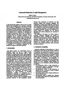
Figure 1-1: Startup-phase QoS system architecture. Oval nodes represent software entities. Rectangular nodes represent data entities. The front- and back- ends of the system are delineated. A dashed oval node is an existing JavaPorts module that is used in conjunction with the newly added software modules i.e. the solid oval nodes........................................... 5 Figure 2-1: (a) An Application Task Graph (ATG) example; (b) the corresponding JPCL textual description; (c) the corresponding AMTP data structure representation............................... 14 Figure 2-2: (a) The ATG for a Manager-Worker example; (b) code snippet showing how the Manager and the Worker components may use the anonymous JP message passing API to exchange messages................................................................................................................ 15 Figure 3-1: (a) The basic JPVTC task modeling elements and their symbols. (b) A task graph modeling nested loops that contain an AsyncWrite element with ports and keys depending on the loop indices. (c) A task graph modeling an AsyncRead loop. .................................... 33 Figure 3-2: (a) A valid (connected and acyclic) behavioral task graph; (b) the corresponding linked list data structure; (c) the XML textual representation for the behavioral graph of Figure 3-1(b) ......................................................................................................................... 35 Figure 3-3: (a) High level overview of the proposed performance estimation and deadlock detection method; (b) the task states transition diagram. ...................................................... 38
xiv
Figure 3-4: (a) Overview of the queuing delays estimation algorithm, (b) example of how the algorithm is applied to a machine queue with three elements. .............................................. 42 Figure 3-5: Port lists and message passing operations modeling: (a) Tasks pseudo code; (b) tasks behavioral graphs; (c) initial port lists; (d) port lists upon visiting the AsyncWrite operations in the Manager graph; (e) port lists upon visiting the SyncWrite operations in the Workers graphs. See text for details. ................................................................................................... 45 Figure 3-6: An example showing the order in which task graph elements enter the machine queue. ............................................................................................................................................... 47 Figure 3-7: Synchronization events handling: (a) a behavioral graph that includes a SYNC element (SyncRead), (b) two different time dependent synchronization scenarios (see text for details). .................................................................................................................................. 48 Figure 3-8: Resolving synchronization events. .............................................................................. 50 Figure 3-9: (a) A conditional block and the state of the probability stack after visiting the second beginIf; (b) nested loops and the state of the iterations stack after visiting the second beginLoop; (c) a loop within a conditional block and the state of the probability and iterations stacks after visiting the beginIf and beginLoop respectively; (d) a SyncWrite within a loop block and the state of the iterations stack after visiting the beginLoop........... 52 Figure 3-10(a) 4-port circuit model example, and (b) the application task graph for a Manager and four Workers configuration. .................................................................................................. 57 Figure 3-11: (a) Manager component pseudo code;(b) behavioral graph for Manager task; (c) Workers component pseudo code; (d) behavioral graph for Worker tasks. .......................... 59 Figure 3-12: (a) results of Exp1, (b) results of Exp2, (c) results of Exp3, (d) configurations used in Exp3, (e) results of Exp4, and (f) configurations used in Exp4. In all cases the estimated and measured results were very close. See text for details. .................................................. 63 Figure 3-13: Exp5: (a) Measured, and (b) Estimated execution time as W, L increase; (c) the relative error distribution, (d) the relative error did not exceed 8%. ..................................... 64 xv
Figure 3-14: Exp5: (a) Simulation time as W, L increase, (b) the simulation time is proportional to WL2. ....................................................................................................................................... 64 Figure 3-15: A snapshot of the performance estimator summary report for the run of the (W=4, L=128) case in Exp5. ............................................................................................................ 66 Figure 4-1: (a) A typical network topology. (b) The FCCG for the machines in (a). In (b), the dashed circles represent clusters, the solid circles represent machines, and the solid lines represent links. ...................................................................................................................... 69 Figure 4-2: The pseudo code for the clustering algorithm. ............................................................ 71 Figure 4-3: A value in a class must not be less or greater than X% of the class mean. ................. 72 Figure 4-4: (a) ATG for a Manager-Worker application; the dashed rectangles represent logical machines, the solid rectangles represent tasks, and the solid lines represent the peer-to-peer logical links between the tasks. (b) The behavioral graph for the Manager task, and (c) the behavioral graph for a Worker task. ...................................................................................... 76 Figure 4-5: (a) The ALMG for the ATG and tasks behavioral graphs of Figure 4-4, and (b) the nodes and edges of the ALMG are annotated based on the CompAmounts and CommSizes of the codeSegments and Write elements in the Manager-Worker behavioral graphs shown in Figure 4-4(b) and Figure 4-4(c) respectively. ....................................................................... 76 Figure 4-6: Pseudo code for the AMH algorithm. ......................................................................... 80 Figure 4-7: The QoS monitoring modules configuration. The solid boxes represent JP tasks, the dashed boxes represent machines, and the solid lines represent the logical links between the corresponding peer-to-peer ports. ......................................................................................... 83 Figure 4-8: Estimating the throughput of any message size based on: (a) two, or (b) four measured points. .................................................................................................................... 87 Figure 4-9: QoS GUI: (a) The Setup QoS System Tab, (b) the QoS System Setup dialog, (c) the Open Application Tab, and (d) measured data log report, see text for details. ..................... 89 Figure 4-10: (a) QoS Session dialog, (b) QoS session results report. ............................................ 90 xvi
Figure 4-11: Concurrent application: (a) its ATG, and (b) from left to right the behavioral graphs for tasks T2, T1, and T3, respectively. .................................................................................. 94 Figure 4-12: Concurrent-overlapped application: (a) its ATG, and (b) from left to right the behavioral graphs for tasks T2, T1, and T3, respectively. .................................................... 94 Figure 4-13: Pipeline application: (a) its ATG, and (b) from left to right the behavioral graphs for tasks T1, T2, and T3, respectively. ....................................................................................... 94 Figure 4-14: The (1-CDF) plots of the WH computation time over the AMH time in both experiments. .......................................................................................................................... 98 Figure 4-15: The average proximity of the WH and AMH heuristics to the optimal in: (a) experiment 1, and (b) experiment 2. ..................................................................................... 99 Figure 4-16: The mean computation times of the WH and the AMH heuristics in: (a) experiment 1, and (b) experiment 2. ...................................................................................................... 100 Figure 5-1: (a) A sample Manager-Worker ATG. (b) The JavaPorts middleware layer stack. ... 103 Figure 5-2: The application configuration that is used to discuss the runtime-phase QoS middleware architecture. ..................................................................................................... 105 Figure 5-3: The runtime-phase QoS middleware architecture and the interactions between various threads and objects to collect QoS related data, and (b) interactions between user task T2 and its QoSService object, and between the QoSService object and the shared QoS data objects during a service request. Circular nodes represent threads, solid rectangles represent objects, and dashed rectangles represent machine boundaries. The arrow directions indicate the type of read/write interaction between threads and objects (e.g. the QoSManager on M2 writes to its LocalQoSData object and reads from the LocalQoSData object on M1, while the API methods of the QoSService object read data from the local and global QoS data objects on M2 and M1 respectively and they return the retrieved data to task T2). ........... 106
xvii
Figure 5-4: The various interactions between user task T2 and its QoSService object, and between the QoSService object and the shared QoS data objects when the GetTaskView() and GetAppView() methods are invoked. ................................................................................. 109 Figure 5-5: A sample JP task template that includes QoS middleware initialization and release code, as well as QoS API method invocations examples. ................................................... 110 Figure 5-6: A sample QoSSetup.txt file. ...................................................................................... 110 Figure 5-7: Steps needed to initialize a task’s QoSService object, launch a QoSManager module, and initialize the shared QoS data objects. .......................................................................... 111 Figure 5-8: The core of a QoSManager thread. ........................................................................ 112 Figure 5-9: The pseudo code for the waitForAnEvent() method. ................................................ 114 Figure 5-10: Estimating the throughput of any message size. ..................................................... 116 Figure 5-11: The application configuration that is used to discuss the token passing algorithm. 119 Figure 5-12: Steps needed to release a task’s QoS modules. ....................................................... 122 Figure 5-13: QoS API methods to get a machine or task state. ................................................... 124 Figure 6-1: (a) static workload with a maximum of 1 (i.e. one DFT task continuously running on the machine), (b) static workload with a maximum of 2 (i.e. two DFT tasks simultaneously and continuously running on the machine), (c) variable workload with a maximum of 1 and a delay of 6 seconds (i.e. one DFT task continuously running every other 6 seconds on the machine), and (d) variable workload with a maximum of 2 and a delay of 6 seconds (i.e. two DFT tasks simultaneously and continuously running every other 6 seconds on the machine). ............................................................................................................................................. 128 Figure 6-2: Manager-Worker application with two workers. ...................................................... 128 Figure 6-3: Self-scheduling (Request) Manager-Worker programming paradigm; The pseudo code for the: (a) Manager task, (b) Worker tasks, and (c) MCT heuristic. ......................... 130 Figure 6-4: The pseudo code for the application used in case2: (a) Manager, (b) Worker, and (c) calcL() method code. .......................................................................................................... 137 xviii
Figure 6-5: The pseude code for fault-tolerant Manager-Worker application: (a) Manager code, (b) Worker code, and (c) the getReadyWorkerPort() method (see text for details). ........ 141 Figure 6-6: The SPMD application configuration ....................................................................... 143 Figure 6-7: The code for the SPMD application template. .......................................................... 143 Figure 6-8: Querying the XView data from: (a) the manager, and (b) from the workers ............ 146 Figure 6-9: The time the QoS Manager on the MASTER machine takes to: (a) measure and record its machine’s attributes, and (b) collect and store the peer machine attributes in the Local/Global QoS data objects on its machine. .................................................................. 147 Figure 6-10: The time the QoSManager on the MASTER machine takes to update the link data when the number of probes per measurement point is set to: (a) two, and (b) three........... 149
xix
List of Tables
Table 2-1: Feature comparison between our QoS management system and related systems. ....... 25 Table 3-1: The basic JPVTC task graph elements and their attributes. ......................................... 33 Table 3-2: Formulas used to estimate the execution delay of task graph elements. ...................... 42 Table 4-1: The static/dynamic machine attributes measured by the QoS monitors. The attribute definitions as well as the UNIX/Linux commands used to measure each attribute. ............. 86 Table 4-2: Task and resource parameters ...................................................................................... 95 Table 5-1: The order of updating the attributes of the links shown in Figure 5-11 and how the token is passed during the first token passing cycle............................................................ 120 Table 5-2: The order of updating the attributes of the links and how the token is passed during the first token passing cycle when the machines in Figure 5-2 are ordered as follows (a) M1, M2, then M3, (b) M2, M3, then M1. ................................................................................... 120 Table 6-1: The various load conditions used in case # 1. ............................................................ 132 Table 6-2: Comparison between the results of the OLB and MCT heuristics under the load conditions in Table 6-1........................................................................................................ 132 Table 6-3: The various load conditions used in case # 2. ............................................................ 133 Table 6-4: Comparison between the results of the OLB and the modified KPB heuristics under the load conditions in Table 6-3 .......................................................................................... 133
xx
Table 6-5: Homogeneous machines under Load1 and W = 6: (a) average elapsed times in minutes, and (b) difference between the non-adaptive and adaptive results. ...................... 138 Table 6-6: Homogeneous machines under Load2 and W = 6: (a) average elapsed times in minutes, and (b) difference between the non-adaptive and adaptive results. ...................... 138 Table 6-7: Homogeneous machines under Load3 and W = 6: (a) average elapsed times in minutes, and (b) difference between the non-adaptive and adaptive results. ...................... 139 Table 6-8: Heterogeneous machines under Load1 and W = 6: (a) average elapsed times in minutes, and (b) difference between the non-adaptive and adaptive results. ...................... 139 Table 6-9: The QoS system overhead as seen from the application perspective under Load1, N = 60, and W = 6: (a) average elapsed times in minutes, and (b) the difference between the results when the QoS support is off/on. .............................................................................. 145
xxi
Chapter 1 Introduction and Motivation
In this chapter we define the problem that our research is focusing on. Moreover, we present the motivation, specific aims and significance of our research. Finally, we provide a brief outline of the rest of the thesis.
1.1 Problem Statement Networks of Workstations (NOWs) are an attractive architecture for solving coarse grain computationally intensive problems. The availability of relatively inexpensive workstations and fast communication networks allow NOWs to often offer a better cost/performance ratio than traditional massively parallel supercomputers. The development of software tools to assist programmers model, build and execute efficiently parallel applications will contribute to the rapid growth of NOWs popularity and user base.
In NOWs, the resources (i.e. workstations and networks) are not dedicated (but shared), which makes the system state dynamic. In such an environment, a workstation becomes overloaded when there are several computationally intensive tasks circulating in its ready queues and a communication link becomes saturated when there are several tasks contending for its bandwidth. Hence, the state of a shared resource changes dynamically depending on the workload that is
1
injected into it. The dynamic system state in addition to the fact that the resources are mostly heterogeneous in NOWs implies that a parallelized application, which may gain performance over a sequential implementation when executed on a lightly loaded system (or on a set of fast machines), may not enjoy any speedup when executed on a heavily loaded system (or on a set of slower machines), assuming that the two systems have the same number of workstations.
In such a dynamic and heterogeneous environment, the application developer must be aware of the static and recent past characteristics (i.e. the system conditions before launching the application) of the underlying system in order to try to map the interacting tasks, which form a network computing application, to a suitable set of resources in a way that meets the desired Quality of Service (QoS) requirements (such as total expected execution time, speedup, etc). Moreover, the application is required to be resource-aware during its runtime in order to try to keep satisfying the desired QoS requirements by possibly adapting itself to the varying resource load conditions.
The need for awareness of the system state, during both the startup and runtime phases, complicates the software development cycle of efficient distributed applications. Thus the need for an application-level QoS management system that automates the mapping of tasks onto machines in the startup-phase and also facilitates application adaptation during the runtime-phase becomes apparent. Such a system, allows the developer to focus on the application functionality details rather than on configuration, and to develop applications that try to meet the desired QoS requirements throughout their life cycle.
1.2 Research Specific Aims and Objectives The application-level QoS management activities must occur during two phases in order to meet the developer's specified QoS requirements throughout the lifetime of an application that is to be 2
executed in an environment where the resources are mostly heterogeneous and the system state is dynamic. The two phases are: startup (i.e. just before the application is launched) and runtime (i.e. during the execution of the application). Our research had two Specific Aims (SA) that focused on exploring the methods that are needed to define and implement the required QoS management activities in each phase. The two specific aims are: •
Specific Aim 1 (SA-1): Design, implement and validate methods and a system to support application-level QoS management activities during the application startup phase.
•
Specific Aim 2 (SA-2): Propose, develop and validate an application-level QoS service for performance and fault-tolerance driven application adaptation at runtime.
The startup and runtime QoS management components are developed in the context of the JavaPorts project [1-5]. JavaPorts is a component framework and a set of tools for the rapid prototyping of parallel and distributed applications executing on NOWs. It facilitates the modeling, configuration, development and deployment of network computing applications. The newly added QoS management components are designed to meet the following objectives: •
Support distributed coarse grain parallel computing applications consisting of a network of interacting tasks executing on NOWs. In a parallel computing application, the tasks can be assigned to different machines (i.e. be distributed), and more than one task can be allocated to the same machine (i.e. multitasking). Furthermore a task may spawn several threads and may contain message-passing operations.
•
Enable the developer to perform what-if performance investigations of different distributed and multitasked configurations before any application coding is attempted.
•
Allow the application developer to run various QoS management sessions in order to automatically find a tasks-onto-machines mapping (application configuration) that meets user defined QoS requirements before the application is launched.
3
•
Provide the capability to obtain suitable QoS services, during runtime, that make the application aware of the current state of used resources (i.e. resource-aware application), and enable it to possibly adapt itself to the varying resource load/state conditions in order to keep satisfying its QoS demands throughout its life cycle.
1.3 Startup Phase QoS Management System (SA-1) The startup phase QoS management system enables the application developer to: (1) run QoS management sessions before the application is launched in order to automatically find a tasksonto-machines mapping that satisfies user defined QoS levels in terms of execution time or speedup ratio; (2) perform what-if performance investigations of various distributed application configurations before any coding is attempted.
1.3.1 Overview The basic features of a startup-phase QoS management system are: (1) application modeling, (2) resource monitoring, (3) a performance estimation method, and (4) a mapping strategy. The resource monitoring system is required to provide information on the dynamic state of the resources. The performance estimator is used to predict the overall running time of an application configuration based on the application model and resources information. A scheduler considers user requirements and constraints as well as the mapping strategy to find acceptable configurations i.e. tasks-onto-machines mappings that meet the desired QoS demands.
Our startup phase QoS management system (see Figure 1-1) consists of front- and back-end subsystem. The front-end subsystem modules provide an interface between the user and the backend subsystem modules. They are user-friendly graphical tools that a developer can use to construct network computing application models, build a machines pool, setup the system preferences, launch/terminate the QoS management modules on a NOW, specify QoS
4
requirements and constraints for the application, and run suitable QoS Sessions to automatically find an efficient tasks-onto-machines mapping. At the back-end, the Resource Monitoring Modules measure, and communicate to the QoS Manager, the dynamic resource state information (e.g. the workload of the machines, the throughput of the network links). The QoS Manager makes the resource information accessible to the other modules by storing it in a shared QoS data object. The QoS GUI interacts with a Scheduler in order to accurately; quickly and automatically find if there exists a tasks-onto-machines mapping that satisfies the QoS levels set by the user. The Scheduler uses user requirements and constraints, an efficient mapping heuristic and a Performance Estimator module to find an acceptable mapping. The Performance Estimator uses: (i) a structural top-level model describing how the tasks interact in the application, (ii) a behavioral model for each task involved, and (iii) NOW resource condition related data, and provides an expected performance estimate for the specific mapping under evaluation.
User
QoS GUI
JPVAC
Setup Data
JPVTC
ATG
Task Behavioral Graphs
Front End Back End Static Dynamic Resource Data
Resources
QoS Manager
Local Monitoring Module
Resources
Scheduler
Performance Estimator
Remote Monitoring Module
Remote Monitoring Module
Resources
Figure 1-1: Startup-phase QoS system architecture. Oval nodes represent software entities. Rectangular nodes represent data entities. The front- and back- ends of the system are delineated. A dashed oval node is an existing JavaPorts module that is used in conjunction with the newly added software modules i.e. the solid oval nodes.
5
1.3.2 Contributions The major contributions of this part of our research are listed below: •
A QoS GUI that allows the application developer to configure and manage the QoS Monitoring Modules and run suitable QoS sessions to find a mapping that meets the desired QoS levels in terms of execution time or speedup ratio (refer to section 4.5 for details).
•
A tool to graphically capture the behavior of the tasks that form a distributed and multitasked application, validate the constructed graphs, annotate the graph elements with benchmark data as needed to estimate the application’s performance, link the structural representation of a distributed application to the behavioral representations of its tasks, and generate XML output [82] for the behavioral graphs (refer to section 3.1 for details).
•
A scalable and non-intrusive resource monitoring system that is based on partitioning the machines pool into different clusters according to their communication characteristics. The clusters are considered as a logical representation of the underlying network of machines (refer to sections 4.2 and 4.4 for details).
•
An efficient mapping heuristic to assign a distributed application (i.e. an application that consists of a set of interacting tasks) to a suitable set of resources based on network and application representations (refer to section 4.3.2 for details).
•
A performance prediction method that estimates the overall running time of distributed and multitasked applications running on NOWs based on a hierarchical, two-level, structural-behavioral application representation as well as static and dynamic resource characteristics. The method supports multitasking (more than one task running on the same machine) and takes into account the queuing effects of other applications. Moreover, it accounts for the synchronization delays of message passing operations and
6
detects application deadlock conditions (refer to section 3.2 for an overview of the method).
1.3.3 Significance The significance of this part of our research is summarized as follows: •
The capability to automatically find and evaluate good tasks-onto-machines mappings efficiently while using the latest dynamic system state information allows the distributed application developer to focus on task decomposition and interaction issues rather than on application configuration.
•
The ability to graphically construct structural and behavioral models for distributed and multitasked applications promotes their rapid prototyping on NOWs and allows estimating their performance characteristics under various resource conditions before any coding is attempted.
•
The what-if performance investigations of various parallel processing scenarios promotes the performance engineering activities at an early stage in the development cycle, which helps the application developer understand better the behavior of the application's task graph and possibly leads to more efficient implementations.
1.4 Runtime Phase QoS Service (SA-2) In an environment in which the resource characteristics keep changing, mapping the application tasks onto a suitable set of machines based on resource conditions at startup may not be enough to guarantee the desired QoS requirements throughout the lifetime of the application. Thus, there is a need for a QoS service that allows the application to assess dynamically the state of the underlying resources and to possibly adapt itself to the varying resource characteristics at runtime.
7
1.4.1 Overview The configuration of a JavaPorts application [1] is static i.e. JavaPorts has no support for task migration or application reconfiguration at runtime. Thus, we adopted a runtime application adaptation model that is based on the following assumptions: � The application configuration is fixed at launch time and does not change at runtime. � The application is responsible for selecting the desired execution path(s) based on the results of the services that are provided by a QoS service at runtime. � QoS support is viewed as a service to each application task that ceases to exist after the task is terminated.
Based on the above assumptions, the application-level QoS service is most suitable for, but not limited to, Manager-Worker style applications. In order to support runtime adaptation in such applications, the Worker components must be replicated on multiple machines. Then, adaptation can be accomplished by re-directing the Manager jobs or messages to the Worker(s) that are running on the fastest machines or connected to it via the fastest network links respectively.
The QoS service is associated with middleware that consists of lightweight QoS Managers. The QoS Managers are automatically and transparently configured, launched and terminated along with the application they service. They monitor the state of the machines and links used by the application and provide an application task with QoS services that enable it to easily adapt itself according to the static/dynamic attributes of any of its application's entities (e.g. machines, links, and tasks). Hence, the QoS services allow an application task to adapt for performance (e.g. CPU speed, link throughput) and fault tolerance (machine and task faults) at runtime. Furthermore, the QoS service is made available to a task via a QoS API that is easy to use and hides all the underlying middleware details from the developer.
8
1.4.2 Contributions The major contributions and deliverables of this part of our research are: •
Lightweight and efficient middleware that only monitors and records the state of the resources used by the application. The QoS support middleware is automatically launched and terminated along with the application it services (refer to sections 5.2 and 5.3 for details).
•
A QoS API that allows an application task to assess and adapt itself to the static/dynamic attributes of its neighboring resources (e.g. peer tasks or machines), or of all the application entities. The QoS API is easy to use but hides all the underlying implementation details from the developer (refer to section 5.1 as well as appendices D and E for details).
1.4.3 Significance The significance of this part of our research is summarized as follows: •
The services to support adaptation for performance allow a task to observe resource load conditions, at runtime, in order to try to keep satisfying the desired QoS requirements throughout its life cycle by sending the jobs or messages to the tasks that are running on the best machines (e.g. machines with best CPU speeds) or are connected by the best network links (e.g. links with best throughput) respectively.
•
The services to support adaptation for fault tolerance allow a task to avoid deadlock and to be more robust by sending the jobs to only responding tasks.
1.5 Thesis Outline In chapter 2, we provide an overview of the JavaPorts framework in which the startup- and runtime-phase QoS management components are integrated. Moreover, we discuss some of the current projects that are relevant to our research. 9
In chapters 3 and 4, we discuss the various software modules and algorithms used to implement the startup phase QoS management system shown in Figure 1-1. In chapter 3, we provide an overview of the JavaPorts behavioral modeling and performance estimation methodologies. In addition, we introduce a graphical tool that is used to capture the behavior of each of the tasks that form the application. Moreover, we present a performance estimation and deadlock detection method used by the Scheduler to evaluate the performance of a given application configuration. Finally, we discuss several experiments conducted to validate the accuracy of the application models and performance estimation method.
In chapter 4, we continue the discussion of the software modules that form the startup phase QoS management system. We present an algorithm to partition the machines pool into different clusters according to their communication characteristics. A fully connected clusters graph is considered as a logical representation of the underlying NOW as well as a basis for a scalable resource monitoring system. In addition, we discuss an efficient mapping heuristic to assign tasks onto machines based on network and application representations. Moreover, we show the implementation details of the scalable and non-intrusive QoS monitoring system. Furthermore, we introduce the QoS GUI that allows the developer to manage the QoS modules and run suitable QoS sessions to find an acceptable mapping. Finally, we demonstrate the efficiency of our mappings using three classes of distributed applications.
In chapter 5, we present the QoS service and its associated middleware. We define the QoS services that are provided to a client task to enable application-driven adaptation for performance and fault tolerance. Moreover, we categorize and introduce the QoS API methods that a task can use to access the supported services. In addition, we provide an overview of the associated QoS middleware architecture. Also, we discuss the initialization, implementation and termination details of the various QoS middleware modules. 10
In chapter 6, we present experiments conducted to validate the runtime QoS service introduced in Chapter 5. We show how the QoS API can be easily used to implement job and application-level schedulers in order to find schedules that outperform their resource unaware counterparts. Moreover, we discuss a Manager-Worker application that uses the QoS API to adapt for Worker faults. Furthermore, we measure the QoS middleware overhead and show that it has minor impact on the performance of the application it services.
In chapter 7, we summarize our work, state our conclusions, and point to new interesting future directions related to supporting QoS management activities during the startup and runtime phases.
11
Chapter 2 Background and Related Work
The startup phase QoS management system as well as the runtime phase QoS service and middleware are developed in the context of the JavaPorts project. Therefore, in this chapter, we present the aspects of the JavaPorts framework that are relevant to the development of these components. Moreover, we survey the existing projects, which are closely related to our research, and discuss their similarities/differences to our work.
2.1 The JavaPorts Framework JavaPorts (JP) [1-4] is a component framework and a suite of tools for the rapid prototyping of distributed Java and Matlab applications executing on NOWs. JP facilitates the modeling, development, configuration, and deployment of coarse grain parallel and distributed applications. The JP framework provides the user with abstractions and APIs that enable anonymous message passing between tasks while hiding the inter-task communication and coordination details. In addition, a unique feature of JP is that it allows in the same application the co-existence and interaction of reusable Java and Matlab components.
A JP application is a set of distributed tasks and its structure can be described using an Application Task Graph (ATG) abstraction. ATG nodes represent tasks and edges represent task-
12
to-peer-task connections. The ATG can be considered as the top (structural) level in a hierarchical, two-level, application representation. Tasks are eventually allocated to machines and several tasks may share the same machine (multi-tasking). The tasks-to-machines mapping can be easily modified using JP, which allows the application user to re-distribute the load at compile time without the need to re-code any part of the application tasks (location transparency). Each task has its own predefined input-output communication ports. Two tasks may exchange messages via an edge (point-to-point connection) using two peer ports (edge terminals). Each task is associated with either a Java or a Matlab software component and several tasks may share the same component implementation [3, 4].
The JP ATG can be captured either textually, using the JP Configuration Language (JPCL), or graphically using the JavaPorts Visual Application Composer (JPVAC) tool [5]. The application ATG is represented internally as an Application-Machine-Task-Ports (AMTP) tree data structure with four levels. An example of an ATG generated using the JPVAC tool is provided in Figure 2-1(a). The corresponding JPCL textual description and AMTP tree data structure are shown in Figure 2-1(b) and Figure 2-1(c), respectively.
The JP Application Configuration Toolset (JPACT) is used to generate Java or Matlab code templates (executable code skeletons) for every task defined in the ATG (based on the parsed configuration file) and to generate scripts (currently Solaris and Linux clusters, with and without NFS are supported) for compiling and automatically launching the distributed application from a designated machine (MASTER machine) in the network. The user needs to add application specific code to complete the automatically generated templates. The generated scripts can be used to compile the completed templates and to launch the distributed application from the MASTER machine (M1 in the example of Figure 2-1).
13
AppName
BEGIN CONFIGURATION BEGIN DEFINITIONS DEFINE APPLICATION "Example" DEFINE MACHINE M1="mach1" MASTER DEFINE MACHINE M2="mach2" DEFINE MACHINE M3="mach3" DEFINE TASK T1="Manager" NUMOFPORTS=2 DEFINE TASK T2="Worker1" NUMOFPORTS=1 DEFINE TASK T3="Worker2" NUMOFPORTS=1 MATLAB END DEFINITIONS BEGIN ALLOCATIONS ALLOCATE T1 M1 ALLOCATE T2 M2 ALLOCATE T3 M3 END ALLOCATIONS BEGIN CONNECTIONS CONNECT T1.P[0] T2.P[0] CONNECT T1.P[1] T3.P[1] END CONNECTIONS END CONFIGURATION
Example
M3
M1
M2
mach3
mach1
mach2
T3
T1
T2
Worker2 Matlab
Manager Java
Worker1 Java
P[1] T1.P[1]
P[1] T3.P[1]
P[0]
P[0]
T2.P[0]
T1.P[0]
(a) (b) (c) Figure 2-1: (a) An Application Task Graph (ATG) example; (b) the corresponding JPCL textual description; (c) the corresponding AMTP data structure representation.
A JP task may use anonymous message passing to communicate with another peer task. In anonymous communications the name (and port) of the destination task does not need to be mentioned explicitly in the message passing method [1]. JP maintains a port list data structure for each port, used to buffer incoming messages. Each port list has different elements, which are uniquely identified by message keys. Hence the message key is used to identify the port list element when writing/reading a message. There are four allowed communication operations in JP, summarized below:
public Object AsyncRead (int MsgKey): Does not block the calling task. Returns a handle to a message if the message has already arrived at the port list element with the specified key, otherwise it returns null.
public void AsyncWrite (Object msg, int MsgKey): Does not block the calling task. Spawns a new thread to transfer and store the message in the receiving task's port list element with the specified key.
14
public synchronized void run (){ // send message to worker port_[1].AsyncWrite(message, key1); // get message from worker message = (Message)port_[1].SyncRead(key2); }
Manager
public synchronized void run (){ // get message from manager message = (Message)port_[0].SyncRead(key1); // send message to manager port_[0].SyncWrite(message, key2); }
Worker
(a) (b) Figure 2-2: (a) The ATG for a Manager-Worker example; (b) code snippet showing how the Manager and the Worker components may use the anonymous JP message passing API to exchange messages.
public Object SyncRead (int MsgKey): Blocks the calling task until a message arrives at the port list element with the specified key.
public void SyncWrite (Object msg, int MsgKey): Blocks the calling task until the sent message is read from the receiving task’s port list element with the specified key.
In Figure 2-2(a), the ATG for a Manager-Workers application is shown. In Figure 2-2(b), two code snippets are provided to demonstrate how the JP anonymous message passing API can be used to exchange a message (The Manager task is also connected via port[0] to another Worker task, not shown in Figure 2-2(a)). The Manager first calls the non-blocking AsyncWrite method on its own port[1], which will result in adding a message personalized by key1 to the corresponding list element of the peer port[0] of the Worker task. Then the Manager waits synchronously to read a message expected to arrive in the key2 element of its own port[1] list. On the other side, a Worker task synchronously waits to read a message from the key1 element of its own port[0] list. Upon receiving this message it calls the blocking SyncWrite operation on its port[0], which results in adding a message in the key2 element of the Manager's port[1] list. The
15
blocked Manager (at the SyncRead) and Worker (at the SyncWrite) are released when the Manager reads the message identified by key2 from its corresponding port[1] list element.
Previously, the developer was responsible for manually specifying the machines on which the JP tasks will be launched. Currently, the developer can use the startup phase QoS system to automatically find a task-onto-machine assignment that is expected to satisfy the desired QoS requirements. Moreover, the runtime-phase QoS service provides a JP task with a QoS API that enables it to query the state of the underlying resources in order to keep meeting its QoS demands by possibly adapting its behavior accordingly. Similarly to the currently used JP Port API, the QoS API uses anonymous communications to preserve task locations transparently.
2.2 Related Work 2.2.1 Startup Phase QoS Management The existing QoS management systems can be categorized into two types: (1) resource monitoring and management systems and (2) scheduling frameworks. The resource management systems provide services to the scheduling frameworks. They monitor and record the characteristics of the underlying resources (workstations, network links, etc). In addition, they make the resource information (e.g. CPU speed, link throughput) available to an application-level scheduler, via an API, to influence the mapping decisions. Moreover, they may provide a scheduler with services (e.g. resource discovery, job submission, check pointing, job migration, security) to execute the application on the best-found resources.
On the other hand, the objective of a scheduling framework is to automatically find a tasks-ontomachines mapping the meets the desired QoS preferences at startup time. The basic components of scheduling frameworks are: (1) mapping heuristic, (2) performance estimation method, (3)
16
application model, and (4) resource information. A scheduler uses the mapping heuristic to find an acceptable tasks-onto-machines assignment. The performance estimator predicts the overall running time of a given mapping based on the application model as well as the resource information. The scheduler uses the performance estimate to decide whether the mapping satisfies the desired QoS demands. These frameworks may rely on their own, or on third party, resource monitoring or management systems to obtain the resource information or to execute the application tasks on distributed machines.
In the sequel, we provide an overview of some of the existing resource management and application-level scheduling frameworks. Moreover, we compare the developed startup-phase QoS management system with the existing systems.
• Resource Monitoring and Management Systems The Network Weather Service (NWS) [10] is a resource monitoring system that periodically measures the dynamic attributes of network and computational resources. It includes software sensors to measure the attributes of machines (e.g. CPU speed, workload, free memory size) as well as end-to-end TCP/IP network links (e.g. throughput and latency). It also uses numerical methods to forecast what the resource conditions will be in the near future. Moreover, it provides a network-level API that static or dynamic schedulers may use to access the gathered resource information.
Similarly to the NWS, the REsource MOnitoring System (Remos) [25-27] is designed to provide a scheduler with dynamic machine and link data. It supports flow and topology queries to obtain the attributes of the resources along an end-to-end communication path and to get a dynamic view of a set of networked machines respectively. It performs the link measurements at the TCP/IP
17
level and can discover the whole network topology. Furthermore, it provides client applications with a network-level API to obtain the dynamic resource attributes.
The Globus Toolkit [11, 12] is a set of software components and tools that provide a variety of core services (e.g. resource discovery, file and data management, information infrastructure, fault detection, security, portability) for grid-enabled applications. It is considered as an enabling technology for the Grid, since it allows users to share various computing and data storage resources securely across geographic and other boundaries without sacrificing local autonomy. Moreover, it provides the Grid Resource Allocation and Management (GRAM) [67] service to facilitate remote job submission and control. GRAM is not a scheduler, but it is often used as a front-end to schedulers. It provides a uniform interface to heterogeneous compute resources that span multiple administrative domains (i.e. Grid-wide and local-area resources). Furthermore, it supports basic Grid security mechanisms, reliable job execution, job status monitoring and job signaling (e.g. stop, restart, kill).
In addition, the Globus Toolkit includes the Monitoring and Discovery System (MDS) [11], which is mainly used by static as well as dynamic schedulers. It consists of a set of services that implement standard interfaces (e.g. WS-ResourceProperties [81]) to publish and access XMLbased [82] resource properties. An Index service collects resource data from registered information sources (e.g. a third party monitoring system such as the NWS) and publishes that information as resource properties. Client applications use the WS-ResourceProperties query interface to retrieve information from an Index.
We have implemented a scalable and non-intrusive resource monitoring system (described in section 4.4) to collect the static/dynamic attribute values of the machines in a pool (e.g. CPU speed, workload, free memory, swap sizes, etc) as well as of the network links interconnecting 18
the machines (e.g. throughput and latency). The JavaPorts framework is used to deploy the monitoring modules on machines within the same administrative domain (e.g. local-area NOW). Our system performs the link measurements at the same level as the JavaPorts message passing operations i.e. at the application-level, which leads to more accurate performance predictions because these operations are implemented in a middleware layer on top of the Java Remote Method Invocation (RMI) [80] layer. On the other hand, systems such as the NWS [10] and Remos [25] perform the link measurements at the network level (i.e. TCP/IP level), which results in more optimistic performance estimates because they do not account for the RMI overheads. However, unlike our monitoring system, the NWS and Remos can monitor the state of various heterogeneous resources across administrative domains.
•
Application-level Schedulers
Our research has been inspired by the Application Level Scheduling (AppLeS) [6-9] project. AppLeS is an agent-based system in which agents try to find an application mapping that satisfies the user specifications based on equation based performance models (describing the behavior of an application that consists of a set of interacting tasks) as well as static and dynamic resource information. It consists of an active agent called the Coordinator and four subsystems, which are: the Resource Selector, the Planner, the Performance Estimator, and the Actuator. The four subsystems share a common information pool that consists of: QoS requirements and preferences provided by the user, model templates to be used by the performance estimator, and dynamic information and forecasts of the system state supplied by the NWS [10]. The Resource Selector selects a set of possible resource configurations based on: user, resource and application information. The Planner, in conjunction with the Performance Estimator and the NWS, computes a potential mapping for each possible resource configuration using predictive models from a model pool. The Coordinator considers the performance of each candidate schedule and selects a mapping that meets the user’s requirements for implementation. Finally, the Actuator 19
interacts with a resource management system (e.g. Globus [11]) in order to schedule the selected application mapping.
The Grid Application Development Software (GrADS) [51, 52] runs on top of Globus [11] to facilitate application scheduling, launching and runtime adaptation. A Resource Selector queries the Globus MDS [11] to get a list of machines in the GrADS testbed and then contacts the NWS [10] to get the dynamic attributes of the machines. The Performance Modeler uses resource information as well as a skeleton based execution model (built specifically for an application that consists of a set of interacting tasks) to map the application to machines. Upon approving a mapping by a Contract Developer component, the Launcher launches the jobs on the given machines using the Globus job management mechanism GRAM [67]. It also spawns a Contract Monitor component to monitor the application’s progress. In addition, the Rescheduler component is launched to decide when to migrate a job to a better machine. Moreover, the application can make calls to a Stop Restart Software (SRS) package that is built on top of MPI [78] to checkpoint data, to be stopped at a particular point, to be restarted later on a different configuration of machines, and to be continued from a previous point of execution.
Condor [13, 14] is a specialized framework to schedule independent, or dependent, computeintensive jobs. It consists of: a job queuing mechanism, scheduling policy, priority scheme, as well as resource monitoring and management modules. Condor places the submitted jobs in a ready queue and then decides when and where to run the jobs according to some scheduling policy. After allocating the jobs onto machines, it monitors their progress and provides the user with their status. Moreover, it supports check pointing as well as job migration. Furthermore, Condor is integrated with Globus (Condor-G) to support batch scheduling on the Grid [96]. In Condor-G, Globus provides protocols for secure inter-domain communication and Condor provides job submission, allocation, and recovery. 20
Legion [15] is middleware that combines heterogeneous resources (e.g. networks, workstations, supercomputers) into a virtual machine that hides different architectures, operating systems, and physical locations from the user. The user can efficiently execute parallel applications on this virtual machine without worrying about different languages, conflicting platforms, or hardware failure. The Legion scheduling module consists of three major components: Collection, Scheduler, and Enactor. The Collection interacts with resource objects to collect the dynamic attributes of computational and storage resources (Legion has no support for network resources yet). The Scheduler selects a set of available resources that match the user’s requirements. Then, it passes the list of selected resources to the Enactor for implementation. The Enactor tries to reserve the desired resources and then sends the results back to the Scheduler. If the results are acceptable to the Scheduler, the Enactor proceeds to submit the application jobs on the resources.
The QoS management system we have developed is suitable for distributed and multitasked, coarse grain, network computing applications. An application task may contain asynchronous or synchronous read and write message-passing operations and it may spawn new threads. The AppLeS [6] and GrADS [52] frameworks as well as methods such as those in [47-49, 76, 77] are similar to our system in that they support the mapping of an application that consists of a network of communicating tasks to NOWs. AppLeS and GrADS, however, do not support the very realistic situation arising in large scale computing in which more than one of the tasks are allocated to the same machine (i.e. multitasking). Our system supports any type of interactions between application tasks via anonymous message passing operations (synchronous and asynchronous). The approach in [47, 77] supports only three application classes namely: concurrent, concurrent-overlapped, and pipeline. Moreover, the method introduced in [48] does
21
not allow asynchronous message passing operations in the tasks. Furthermore, the work discussed in [49] is only suitable for Manager-Worker type of applications.
On the other hand, scheduling frameworks such as Condor [14], Legion [15], MSHN [16], SmartNet [73], and MAP [75] can map a set of independent jobs from different users onto a heterogeneous suite of machines. They also can map a set of inter-dependent tasks represented by Directed Acyclic Graphs (DAGs). A DAG is considered as a structural application representation in which nodes represent tasks and edges represent the tasks inter-dependencies. However, unlike our system, these systems cannot evaluate the performance of an application that consists of a set of interacting and communicating tasks.
Other end-to-end QoS management systems, such as those in [59-66], are designed to support multimedia applications. Since multimedia applications are very communication intensive, these systems mostly provide flow services rather than processing services, which are usually required by a coarse-grain network computing application. Moreover, these systems reserve the machines and network links along the end-to-end communication path to guarantee the desired QoS levels delivery during a multimedia session. However, reserving the resources for a compute intensive application that may run for several hours is not appropriate, since that defeats the purpose of resource sharing in NOWs.
The performance models used in AppLeS [6-9] and GrADS [52] as well as in methods such as those reported in [37, 38, 42, 43, 74] are equation based, thus the developer is responsible for defining a set of equations that represent application behavior. The equations can be parameterized by application (e.g. benchmark data, problem size, number of iterations) and resource (e.g. CPU speed, link throughput) characteristics. In any case, they are manually defined, which makes the modeling process cumbersome and error prone. Moreover, the 22
developer must fully understand the behavior of the application in order to define accurate performance prediction equations for it. Equation based models may not be suitable to estimate the performance of multitasked applications or of applications that contain anonymous message passing operations. A more detailed survey of existing performance estimation methods for network computing applications is provided in section 3.2.5.
In this dissertation, we developed a graphical tool that allows the developer to easily capture the behavior of the application tasks and to connect the behavioral task models structurally to end up with hierarchical, two-level, application representations (see Chapter 3). The nodes (elements) in a behavioral task graph represent basic code constructs and the edges define the nodes execution order. Most elements in a graph are annotated with benchmark performance data (e.g. execution time of a sequential code block on a reference machine) as needed to estimate the application performance. Thus, in our system the developer does not need to understand how the application performance is estimated because the task behavior is easily defined as a sequence of computation and communication operations. Moreover, our simulation based performance estimation method (described in section 3.2 and in [97]), unlike other existing methods for network computing applications, can account not only for execution, but also for the queuing and synchronization delays of all tasks forming a distributed and multitasked application. Also, it accounts for the contention effects of other applications and it can detect possible application deadlock scenarios.
Our system also uses a scalable mapping heuristic [98] that extends the method discussed in [47] in order to find a tasks-onto-machines mapping the meets the user’s QoS demands. It is more suitable to compare this method to related work in section 4.3.3 after discussing it in Chapter 4.
23
Scheduling systems such as AppLeS [6], Globus [11], and GrADS [52] rely on third party monitoring systems such as the NWS [10] and Remos [25] to obtain the resource information they need. Similarly to our system, Condor [13] and Legion [15] have their own resource monitoring modules. However, Legion only monitors the state of the machines and does not estimate any link attributes. Moreover, unlike our system that performs all link measurements at the application-level, systems such as Condor, NWS and Remos measure the link attributes at the network-level. Hence, our performance estimates can be more accurate than the AppLeS and GrADS estimates.
Although this is not part of this research, but it is important to emphasize that our system uses the JavaPorts framework to deploy the application tasks on the desired machines. JavaPorts provides scripts to deploy an application onto heterogeneous machines that fall within the same administrative domain (i.e. local area clusters of workstations). Similarly to our system, the Legion [15] and Condor [14] systems have their own job submission mechanisms. Conversely, systems such as AppLeS and GrADS rely on third party frameworks, such as Globus [12], for job submission and resource discovery. So, our system is basically a middleware layer that does all the monitoring and servicing behind the scenes, at the application-level, without the support of some underlying resource monitoring infrastructure. This makes it applicable in any NOW that just runs Java/RMI and JavaPorts.
•
Summary
We summarize in Table 2-1 the previous discussion by showing the features that are supported by our startup phase QoS management system and by the most prominent frameworks for grid and cluster computing.
24
Features
Application Modeling
Performance Estimation
Scheduling Heuristics
Resource Monitoring
Job deployment
Other Features
JavaPorts
Yes (structural and behavioral)
Yes (distributed and multitasked)
Yes (application-level)
Yes
Yes (on local-area networks)
NWS
NA
NA
NA
Yes
NA
Forecasting.
ReMoS
NA
NA
NA
Yes
NA
Network discovery.
Globus
NA
NA
NA
Uses NWS
Yes (on wide- and local-area resources)
Resource and data management/discovery, security, and fault detection.
AppLeS
Yes (structural and behavioral)
Yes (distributed)
Yes (application-level)
Uses NWS
Uses Globus or Legion
NA
GrADS
Yes (structural and behavioral)
Yes (distributed)
Yes (application-level)
Uses NWS
Uses Globus
Job migration and adaptation.
Condor
Yes (structural)
NA
Yes
Yes (on wide- and local-area resources)
Resource management and security.
Legion
Yes (structural)
NA
Yes (only machine attributes)
Yes (on wide- and local-area resources)
Resource management and security.
Project
Yes (job scheduler)
Yes (job scheduler)
Termination, message passing API, and QoS API to support adaptation for performance and fault tolerance.
Table 2-1: Feature comparison between our QoS management system and related systems.
2.2.2 Systems for Runtime Adaptation and Application Fault Tolerance Two mechanisms are needed to support application adaptation at runtime, these are: (1) middleware to monitor the dynamic conditions of the resources and the application at runtime, and (2) software modules to make adaptation decisions based on the system and application states as well as user defined QoS requirements. The adaptation decisions can be made by the application itself or by system-level software modules that are transparent to the application. Application-driven adaptation can be accomplished via a QoS API that an application can use to obtain resource/application conditions at runtime in order to keep meeting its QoS demands by adapting itself accordingly. In this case, the developer is responsible for implementing and adding the adaptation code in the application. On the other hand, system-driven adaptation requires 25
software module(s) that run along with the application in order to monitor its progress and to change its behavior when it does not meet the desired QoS levels. In such systems, the application code remains the same (i.e. no adaptation code is added), but the developer is required to edit a QoS profile in order to make the following information available to the system: (1) multiple execution paths for the application, (2) the means by which application progress can be monitored and influenced, and (3) QoS metrics and levels.
We have implemented a QoS Service (discussed in Chapter 5) that enables application-driven adaptation for performance and fault tolerance. The service is associated with middleware to monitor the dynamic state of the application tasks as well as the attributes of the machines and logical links used by the application. Unlike similar QoS APIs, such as the NWS and Remos APIs, our QoS service implements an anonymous and easy to use QoS API, which makes the application code independent from the underlying resources i.e. the application can be configured to run on a new set of machines without any need to modify its code. Moreover, the associated service middleware is automatically configured, launched, and terminated along with the application it is servicing. Furthermore, the middleware is lightweight since it does not provide services to other applications i.e. it does not waste cycles monitoring unused resources.
•
Application-driven Adaptation Frameworks
Similarly to our QoS API, frameworks such as NWS, Remos, and Globus-MDS (discussed previously in section 2.2.1) support an API to enable application-driven adaptation. However, calls to NWS and Remos APIs are not anonymous because they require specifying machine and port information (e.g. machine domain name, server port) in a method call, which requires modifying the source code when the application is allocated to a different set of machines. Furthermore these systems provide services to multiple applications, but they do not provide any services for application fault-tolerance. Moreover, they report optimistic link throughput and 26
latency values because the link measurements are performed at the network and not at the application-level as in our system. But, unlike our QoS service, these APIs can be used to get the information on Grid-wide as well as local-area resources.
•
System-driven Adaptation Frameworks
A framework for automatic adaptation of tunable distributed applications is introduced in [17]. This framework supports applications that can be executed in alternate ways i.e. they have different resource utilization profiles. A tunability interface is supported to provide a way to express the availability of alternate configurations for the application as well as the mechanisms to monitor and influence the progress of the application. Moreover, a monitoring agent monitors the progress of the application and the state of the resources that are used by the application at runtime. In addition, a resource scheduler correlates the measured resource conditions and specified QoS requirements with stored performance models. Furthermore, a steering agent is responsible for reconfiguring the application when needed.
An architectural support for QoS for CORBA [83] Objects (QuO) is introduced in [18, 19]. QuO employs the concept of a connection between a client and object (server), an encapsulation including the desired QoS requirements specified in the form of a contract. A Contract Description Language (CDL) is used to describe the contract between a client and an object in terms of usage and QoS. In QuO, the object is responsible for the end-to-end QoS. Thus it is aware of the system conditions and part of its implementation is moved into the client's address space. A delegate object is used to implement the abstraction of a client-object connection with QoS. QuO provides mechanisms to support the following adaptivity schemes: finish later than expected, do less than expected, and use an alternate mechanism with different system properties. Thus, to allow an application to adapt to changing system conditions, the application developer must be able to deploy multiple implementations of a given object. Callbacks are used to warn a 27
delegate object and a client of a pending request whose expected QoS is not being met, which allows them to either take compensatory action to try to operate within its expectations, or to change those expectations.
A framework that employs JavaSpaces to facilitate adaptive master-worker parallel computing on networked clusters is introduced in [20]. In this framework, the state of worker machines (i.e. average worker CPU utilization) is monitored in order to use that information to drive the scheduling of tasks on workers.
An adaptation framework Adaptive.Net is introduced in [21]. The framework includes a monitoring infrastructure and a runtime environment able to execute dynamic reconfiguration commands. Adaptation is realized in this framework by adding/removing components to/from applications and by migrating components to other hosts in order to change the application configuration such that a pre-defined adaptation policy is satisfied. The adaptation policy defines a mapping of monitored parameters to application configurations.
A real-time adaptive control infrastructure called Autopilot that is built on top of Globus is introduced in [51]. The user specifies a desired performance contract. An Autopilot manager is spawned before launching the application. Parsers are used to locate instrumental code constructs in the application, such as loops or procedure calls, and insert the requisite instrumentation calls to compute start and end times, elapsed times, and log hardware counter data. The Contract Monitor calculates the ratio between the measured execution time and the desired execution time. If the average ratio is greater than a specified tolerance limit, it contacts the Rescheduler to migrate the application to better machines.
28
The AQuA architecture, which is designed to provide adaptive fault tolerance to CORBA applications by replicating objects, is introduced in [22]. All replicas of an object form a group. Different replication schemes are used to ensure that the messages are delivered to the members in a group. The Quality Object (QuO) [18] is used to specify the dependability requirements. A dependability manager configures the application based on reports of faults and QoS requirements of application objects. Moreover, an object factory that runs on each host is used to instantiate and to destroy objects as well as provide information about its host to the dependability manager.
An AFT-CCM model (Adaptive Fault-Tolerance on the CORBA Component Model) for constructing distributed applications with fault-tolerance requirements is introduced in [23]. The model employs adaptive fault-tolerance in a way that is completely transparent to the application. The model consists of software modules that configure, monitor, and replicate application components. Moreover, the modules adapt the application configuration, based on a replication technique, in order to satisfy user-defined QoS levels. Furthermore, the model monitors host and application component faults. A host fault is detected when a Fault Detection (FD) agent on a host stops responding to calls from the Adaptive Fault-tolerance Manager (AFT). In addition, a component fault is detected when a component stops answering calls from the FD agent. Faults are assumed when a call to a FD agent or to an application component results in an exception.
Unlike our QoS service [99], the adaptation in the previous system-driven frameworks is delegated to system-level software modules and is transparent to the application. However, language support, such as the tunability interface discussed in [17], is required to specify alternate behaviors of an individual module as well as QoS metrics and levels, which is not a trivial process. On the other hand, our QoS service is anonymous and simple to use. It allows an application task to easily adapt according to the state of its neighbors or all of the application 29
entities. But, our QoS middleware does not support check pointing, job migration or dynamic addition of tasks at runtime. Similarly to existing system-driven adaptation frameworks, such as [17-22], our adaptation model requires the existence of multiple execution paths for the application to choose from. That is achievable by replicating workers or objects on several machines and then sending a job to the worker on the best machine, or by having alternate configurations that have different resource requirements. For example, a server that is transmitting a video stream to a client can respond to a reduction in available network throughput by compressing the stream or by selectively dropping some frames.
30
Chapter 3 Behavioral Task Modeling and Performance Estimation of Network Computing Applications
In this chapter we provide an overview of the JavaPorts behavioral modeling and performance estimation methodologies. First, we discuss the design of the JavaPorts Visual Task Composer (JPVTC), a set of algorithms integrated into a graphical tool, which can be used in conjunction with the JPVAC tool to construct hierarchical, two-level, structural-behavioral application models. Such models can be used to facilitate QoS negotiations, performance engineering, and rapid prototyping of component-based applications. Then, we present methods for the performance estimation of different application configurations based on application models i.e. before any coding is attempted. These methods can help the application developer understand the expected behavior of the interacting application tasks under different resource conditions and detect potential deadlock situations.
3.1 Behavioral Representation of Distributed Tasks A behavioral task graph consists of nodes (elements) representing basic code constructs and of edges representing dependencies between them. It models the general organization of a task as a
31
sequence of computation and communication elements. A behavioral graph is associated with each application task. Therefore behavioral graphs of tasks can be considered as the second (lower) level, in a hierarchical two-level representation of a distributed and multi-tasked application. The JPVTC is a new tool that we have added to the JavaPorts suite in order to allow developers to construct graphically behavioral models for the tasks of distributed applications. The application models are used to perform what-if performance analysis and QoS evaluations of different task configurations.
In the following subsections we discuss: the basic elements and structures supported by the JPVTC tool, its features and functional modes, the association of structural JP application graphs to behavioral task graphs, the produced XML output when a graph is saved, and the related work.
3.1.1 Basic Elements and Structures used to Build Task Behavioral Graphs In order to capture the behavior of a JP task, the code constructs that contribute to the task's total execution time significantly should be modeled. A JP task may include sequential code blocks, iteration constructs (e.g. for loops), and conditionals (e.g. if statements). Moreover, it may contain synchronous/asynchronous message passing operations and spawn new threads. The JPVTC tool supports the necessary elements for modeling the basic JP code constructs. Most of the elements can be annotated with attributes and benchmark performance data, as needed to estimate the application's performance. The currently supported elements and their attributes are listed in Table 3-1. Each element has its own symbol within the JPCTC tool. A snapshot of the supported elements symbols is provided in Figure 3-1(a).
32
for ( p = 0 ; p < W ; p++ ) { // bloop1 for ( k = 0 ; k < L ; k++ ) { // bloop2 port_[ p ].AsyncWrite( msg , k ) ; } // eloop2 } // eloop1
while ( msg = port_[ p ].AsyncRead( k ) ) { // codeSegment } // while
(a) (b) (c) Figure 3-1: (a) The basic JPVTC task modeling elements and their symbols. (b) A task graph modeling nested loops that contain an AsyncWrite element with ports and keys depending on the loop indices. (c) A task graph modeling an AsyncRead loop.
Element Type codeSegment
Attribute(s) Average execution time
fork beginIf
Probability of entering a block Number of iterations Data size (Kbytes), port, message key Data size (Kbytes), port, message key Port, message key Port, message key Port, message key -
endIf beginLoop endLoop AsyncWrite SyncWrite AsyncRead SyncRead beginAsyncReadLoop endAsyncReadLoop
Comments Sequential code block; In time units on a reference machine. Spawn a new thread. Begin of a conditional block. End of a conditional block. Begin of a loop block. End of a loop block. Non-blocking write. Blocking write. Non-blocking read. Blocking read. Begin of an AsyncRead loop block. End of an AsyncRead loop block.
Table 3-1: The basic JPVTC task graph elements and their attributes.
A unique feature of JPVTC is that it allows modeling loops containing message-passing operations with ports and/or message keys depending on the loop indices (i.e. parameterized ports and keys). For example, in the task graph shown in Figure 3-1(b) the port on which the AsyncWrite method is called and the message key it uses vary in each iteration, depending on the indices of loops bloop1 and bloop2 respectively. The user can model this behavior by specifying these loops in the AsyncWrite element attributes dialog launched by right clicking on the element, as shown in Figure 3-1(b). This kind of loop structure is convenient for modeling a Manager33
Worker parallel computing pattern, in which the load is partitioned among several Workers and the Manager needs to send/receive several personalized messages to/from each Worker. Supporting this type of loops reduces the complexity and size of the constructed graphs, since a loop with a single communication operation is in this case equivalent to a one-to-many communication primitive (scatter).
Another typical structure is the AsyncRead loops and can be modeled in JPVTC using the beginAsyncReadLoop and endAsyncReadLoop elements as shown in Figure 3-1(c). Such a loop is exited when the AsyncRead finds that a message has been deposited in the port’s list element with the specified key. This kind of loop is useful when the parallel application can do some useful work instead of blocking while waiting for a message to arrive.
3.1.2 JPVTC Basic Features and Functional Modes JPVTC consists of a menu bar, a tool bar, and a desktop pane. The menu bar contains menus that provide access to all tool features. The tool bar contains buttons to provide the user with quick access to the most important features. Several internal frames can be opened in the desktop pane to allow editing and viewing multiple behavioral graphs simultaneously. A snapshot of the tool is shown in Figure 3-1(a).
There are five functional modes for constructing/editing graphs in the JPVTC tool. In the add element mode, new elements (nodes) can be added to the graph by simply selecting the element type and clicking on the desired placement location. Elements can be dragged from a location to another in the move element mode. In the delete element mode, an element is removed from the graph by clicking on it. Selecting and dragging an element in the copy element mode results in a new instance of the selected element with its inherited attributes in the location where the mouse is released. In the connect element mode, elements can be connected together by dragging the 34
mouse from a source element to a destination element. In addition, clicking right on an element symbol will launch an attributes form, which allows the user to provide the element's attributes.
Element1 fork1 Attributes Parent * Child1 * Child2 * *
Element2 cs1 Attributes Parent * Child1 * *
Element3 aw1 Attributes Parent * Child1 * * Element4 cs2 Attributes Parent * Child1 * * Element5 cs3 Attributes Parent * Child1 * *
Start
(a) (b) (c) Figure 3-2: (a) A valid (connected and acyclic) behavioral task graph; (b) the corresponding linked list data structure; (c) the XML textual representation for the behavioral graph of Figure 3-1(b)
The behavioral graphs are represented internally using an efficient graph data structure. The data structure is a link list of element instances. An element instance contains the attributes of the element (type, ID, (x, y) coordinates, annotated performance data, etc) as well as pointers to allow easy access to the parent and the children of the element in the list. The element without a parent is considered the first element in the graph (i.e. graph traversal starts from that element). The data structure for the behavioral graph of Figure 3-2(a) is shown in Figure 3-2(b).
An algorithm to check if every begin element has a matching end element is also developed; e.g. a graph with a beginIf and without an endIf is invalid. Moreover, the algorithm considers a graph valid if all of its elements are connected. In addition, a cycle check is also performed on the fly on a graph under construction in order to report and prevent any cycles. A graph contains a cycle, if there is a path that starts and ends at the same element. Furthermore, an algorithm to organize and center a graph in an internal frame is integrated in the tool. 35
A structural (application-level) and various behavioral (task-level) graph models should be linked in order to construct a hierarchical network computing application model. The JPVTC tool supports the association of a behavioral graph to its corresponding application task. Moreover, the JPVAC [5] tool allows annotating a task with its behavioral graph. Hence, the structural and behavioral models can be linked interchangeably in either of the tools.
JPVTC saves the behavioral graphs in an eXtensible Markup Language (XML) format defined in a graph Document Type Definition (DTD) to facilitate the interchange of the graphs. The DTD consists of a list of elements including the behavioral graph elements and an arc element for capturing connectivity information. Every element has a unique identifier. All elements, except the arc element, have a location statement to specify their placement in the internal-frame. In addition, most elements have lists that capture their annotated information and attributes. In Figure 3-2(c) we provide the XML textual representation for the behavioral graph shown in Figure 3-1(b).
3.1.3 Related Work A graphical tool, called HeNCE, was introduced in [28]. HeNCE is built on top of the Parallel Virtual Machine (PVM) package [79]. The tool provides the programmer with a high level abstraction for specifying parallelism. However, the user of the tool will never explicitly write PVM code. In HENCE the parallel application is represented as a directed graph in which the nodes represent subroutines and the arcs represent control flow and data. The tool allows the user to provide multiple implementations of the nodes based on the target architecture. The tool automatically translates the directed graph into an executable PVM parallel application. The programmer can also provide the tool with a cost matrix that can be used to map tasks onto machines. Unlike JPVTC, HeNCE does not provide any constructs to represent the behavior of the application tasks and does not estimate the performance of the application. 36
Another graphical tool, called Zoom, was introduced in [29]. The application representation in Zoom is hierarchical, structural (i.e. at the task level), and network and interface independent. In Zoom, the user can specify communication and data conversion matrices to be used by a scheduling tool. Zoom does not provide any constructs to represent the behavior of the tasks that form the application.
A parallel visual programming tool, called CODE, was introduced in [30]. CODE allows the user to represent the application as a dataflow graph. The graph is automatically translated into executable code. The programmer can specify the nodes firing rules using CODE. The objective of CODE is to translate a dataflow graph into executable parallel code.
The main objective of the previous and other similar tools, such as GRAPNEL [31], SkIE [32], TRAPPER [33], and PVMGraph [34], is to generate executable parallel code from the graphical representation of the application. These tools neither address the performance engineering activities during the application development cycle, nor do they focus on QoS related issues. In addition, they only support the graphical representation of the application's structure and they do not capture the behavior of the individual application tasks.
The tool discussed in [35] focuses on estimating the application's performance and can be used to graphically capture the behavior of the application tasks using Petri Nets (PN) [68] models. This tool as well as several PN based modeling tools, such as GreatSPN [69], HPSim [70], and JFern[71], allow constructing quite complex task behavioral descriptions that may include synchronous/asynchronous message passing operations. However, Petri Nets cannot model anonymous message passing operations and are harder to construct.
37
3.2 Performance Estimation and Deadlock Detection In this section, we present a new method for performance estimation and deadlock detection of multi-tasked and distributed network computing applications. This method can be used to perform what-if performance investigations as well as QoS evaluations of different application configurations in the context of JP. The proposed Performance Estimator module (see Figure 1-1) takes as input: the application's AMTP tree (generated by the JPVAC tool), the task behavioral graphs (constructed using the JPVTC tool), and the static and dynamic resource information (provided by the monitoring modules). The performance estimation method predicts the expected total execution time of the application for the tasks-to-machines mapping defined in the AMTP tree (the evaluation of another mapping requires only the modification of the AMTP tree). It accounts for the execution, queuing, and synchronization delays of all tasks forming the distributed application. START Initialization
Application complete?
YES
NO begin for each machine
NEXT ITERATION OVER QUEUE
NEXT PASS OVER ALL MACHINES
Start
Update machine queue Queue empty?
AGGREGATE
YES
SyncRead or SyncWrite that sent its message visited
NO SYNC and wait?
YES
Last element in graph visited
NO Calculate elapsed time of element(s) in queue
DONE
Synchronization resolved or Schedule parallel threads
SYNC
COMPLETE Expected Message never arrived
end for each machine Resolve SYNC Deadlock?
YES
DEADLOCK
DEADLOCK
NO
(a) (b) Figure 3-3: (a) High level overview of the proposed performance estimation and deadlock detection method; (b) the task states transition diagram.
38
A high level overview of the proposed performance estimation and deadlock detection algorithm is provided by the flowchart of Figure 3-3(a). At initialization time, port list data structures are initialized according to the point-to-point connections between pairs of peer ports specified in the AMTP tree. Port lists are needed to model anonymous message passing operations. In addition, a ready queue is generated for each machine, as needed to model the task element queuing delays. Data structures are also generated for each behavioral task graph. A mapping table that associates each task with the machine on which it is allocated is initialized. The first element in each task behavioral graph is inserted into the appropriate machine queue. Elements of tasks allocated to the same machine are inserted into the same machine queue. The execution time of an element is recalculated, if necessary, by taking into account the static and dynamic information of the corresponding resources, before it is inserted in its queue.
The algorithm loops over all machine queues. A queue is updated (i.e. the elements that completed execution are removed from the queue and the elements that depend on them enter the queue) at the beginning of each iteration. The elapsed times (i.e. queuing and execution delays) of elements in the current queue are calculated at the end of each iteration. The calculated elapsed time of the current iteration is added to the total running time of the corresponding task(s). Then another iteration over the same queue starts. The algorithm exits the loop of a machine ready queue and moves to update the next machine queue when either the current queue becomes empty or a task in it is waiting for a synchronization event to occur. Upon exiting the loops of all machine queues (i.e. upon completion of the current pass), the algorithm tries to resolve any pending synchronization events, checks for deadlocks and exits if one is detected. If the application did not complete, another pass starts by looping over all machine queues once more. This process continues until the application completes or a deadlock is detected. At the end, the estimated application total running time corresponds to the completion time of the task with the longest delay. 39
A task can be in one of the following four states: AGGREGATE, SYNC, DONE, or DEADLOCK, as shown in the task state diagram of Figure 3-3(b). A task is in the AGGREGATE state, if it is not waiting for a synchronization event to occur. A task is in the SYNC state, if a SyncRead element is waiting for a message to arrive or a SyncWrite element that sent its message is waiting for the message to be read. A task is in the DONE state, if all of its model's elements have been executed (visited) and removed from the queue. A task is in the DEADLOCK state, if a waited upon message never arrives at the port list with the specified key. A task has to be in the DONE or SYNC states at the end of a pass. A task that never enters the SYNC state, transitions to the DONE state in one pass (may be after multiple iterations over the queue). On the other hand, a task with synchronization elements needs more than one pass to complete.
The complexity of this algorithm is O(P⋅I⋅M), where P is the number of required passes, I is the expected number of iterations over a machine ready queue for a pass, and M is the number of machine queues. The number of passes depends on the number and order of execution of the synchronization elements (i.e. when there are no synchronization elements in any of the behavioral graphs P=1). The number of iterations is proportional to the expected number of elements in the task behavioral graphs assigned to each machine. The number of queues is the same as the number of machines in the ATG. Usually the number of machines and number of elements per task is not very large, which makes the algorithm scalable.
In the sequel, we elaborate on the most important aspects of the proposed performance estimation algorithm: (1) delay modeling and calculation, (2) updating the machine queues, (3) synchronization events modeling, (4) deadlock detection, (5) conditionals and loops modeling.
40
3.2.1 Delay Modeling and Calculation The total running time of a distributed multi-tasked application includes execution, queuing, and synchronization delays. The execution delay accounts for the actual service time of each one of the basic code constructs in the task behavioral models. The queuing delay is the time that a task spends waiting in the ready queue of a shared machine. The synchronization delay is the time that a blocked message-passing operation spends waiting for an event to occur. All three types of delays should be accounted for accurately in order to estimate the overall running time of a distributed application.
•
Execution time calculation
The calculation of the elements execution time takes into account the annotated performance data, the tasks onto machines mapping, as well as the latest static/dynamic underlying system data. Some elements are annotated with performance data on a reference (benchmark) machine as needed to estimate their execution time. These elements are divided into two groups: the first group includes the codeSegment, beginIf, and beginLoop elements; the second group includes the SyncWrite and AsyncWrite elements.
The codeSegment element is annotated with the expected execution time of the code block it represents on a reference machine (see Table 3-2). Since coarse grain code segments usually correspond to one or more subroutine calls the execution time of a block can be measured on a benchmark (reference) machine (e.g. fastest machine in a cluster) in non-shared mode (i.e. no other applications are concurrently running on the reference machine with the benchmarked code block). If a codeSegment element is part of a task allocated to a slower machine, its execution time is automatically scaled down. Furthermore, in order to account for the potential CPU contention effects of other applications, the codeSegment execution time is also multiplied by a
41
dynamically updated load factor. The QoS Monitoring Agents (see Figure 1-1) are used to estimate the load average of the used machines. Element Type codeSegment fork beginIf endIf beginLoop endLoop AsyncWrite SyncWrite AsyncRead SyncRead beginAsyncReadLoop endAsyncReadLoop where: -
Execution Time (BMS/AMS)*AET*LF 0 0 0 0 0 DataSize/Throughput(DataSize) DataSize/Throughput(DataSize) 0 0 0 0
Dependencies annotation, system data, mapping none none none annotation none annotation, system data, mapping annotation, system data, mapping annotation annotation annotation none
BMS: The reference (benchmark) machine speed (in MHz). AMS: The speed of the machine where the task is allocated (in MHz). AET: The annotated expected execution time on the reference machine (in time units). LF: An average load factor to account for the CPU contention effects of the other applications. DataSize: The annotated message size (in Kbytes). Throughput(DataSize): The estimated throughput of a message with size DataSize over the link between the machines of the peer ports.
Table 3-2: Formulas used to estimate the execution delay of task graph elements. for each machine
cs1
aw1
aw2
RET = 3; ET = 0
RET = 1; ET = 0
RET = 2; ET = 0
Initially
queue.currentTime = 0 numOfElementsInQueue = 3 minRemainExecTime = 1 queue.state = AGGREGATE
for ( each element in queue ) { if ( element.RemainingExecTime == 0.0 ) { - Remove element from queue if ( the element that exited the queue has children ) { - Calculate the execution time of each child element - Insert each child element into the queue } // end if } // end if } // end for .....
cs1
aw1
aw2
RET = 2; ET = 3
RET = 0; ET = 3
RET = 1; ET = 3
At the end of iteration 1
queue.currentTime = 3 aw1 completes and will be removed from queue aw1 overall time = 3 numOfElementsInQueue = 2 minRemainExecTime = 1 queue.state = AGGREGATE
YES if queue empty? NO YES if SYNC and wait? NO
cs1
aw2
RET = 1; ET = 5
RET = 0; ET = 5
At the end of iteration 2
NEXT ITERATION
// minExecTime = minimum remaining execution time of elements in queue - Find minRemainExecTime of elements in queue queue.currentTime = 5 aw2 completes and exits queue aw2 overall time = 5 numOfElementsInQueue = 1 minRemainExecTime = 1 queue.state = AGGREGATE
for ( each element in queue ) { - element.RemainingExecTime = element.RemainingExecTime - minRemainExecTime // ElapsedTime = queuing + execution times - element.ElapsedTime = element.ElapsedTime + ( minRemainExecTime * numberOfElementsInQueue ) } // end for .....
cs1 At the end of iteration 3 RET = 0; ET = 6 queue.currentTime = 6 cs1 completes and exits queue cs1 overall time = 6 numOfElementsInQueue = 0 minRemainExecTime = 0 queue.state = DONE
for each machine
(a) where: -
(b)
ET: Elapsed Time of an element (i.e. sum of queuing and execution delays). RET: Remaining Execution Time. Initially RET = expected execution time of the element. minRemainExecTime: Minimum RET of elements in queue.
Figure 3-4: (a) Overview of the queuing delays estimation algorithm, (b) example of how the algorithm is applied to a machine queue with three elements.
42
The beginIf element is annotated with the probability of entering the conditional code block and the beginLoop is annotated with the number of expected iterations. These attributes are application and not mapping dependent. The average execution time of the SyncWrite and AsyncWrite message passing elements depends on the communication message size and the throughput of the link connecting the machines on which the tasks containing the communication elements are allocated. The monitoring agents measure and record the throughput of the links. The equations used for estimating the execution times of all elements supported by the JPVTC tool based on benchmark data and runtime measurements are summarized in Table 3-2.
•
Queuing delay calculation
Queuing delay estimation (due to multitasking) is based on time sliced scheduling. We assume that the time slot is much smaller than the average execution time of the elements in the queue and the task context-switching overhead is negligible. Based on these assumptions, if there are two elements with the same execution time in a machine queue, the elapsed time (i.e. queuing plus execution delay) of an element is equal to double its execution time (i.e. half of the elapsed time accounts for the time spent waiting in the ready queue and the other half accounts for the actual service time). In order to account for the queuing delays, the elements of multiple threads or tasks that contend for the same CPU are inserted into the same machine queue. In each iteration the algorithm estimates the elapsed times of elements in each machine queue based on the pseudo code of Figure 3-4(a). In the example of Figure 3-4(b), we demonstrate how the algorithm is applied to a queue that contains three elements, a codeSegment (cs1) and two AsyncWrites (aw1 and aw2). In this example, it is assumed that the three elements in the queue have no children, hence no other element will enter the queue.
43
•
Synchronization delay calculation
The performance estimation scheme mimics the JP port lists in order to be able to account for synchronization delays and model accurately the behavior of the message passing operations supported by the JP communication API. At the initialization phase, the performance estimation algorithm builds port lists for each task based on information available in the AMTP tree. The algorithm adds a message to the corresponding port list dynamically based on the specified port and key of the visited operation. When an Async/Sync write operation is visited, it adds a message to the peer port list with specified key. The message is stamped with the time the write operation completes sending the message to model message transmission according to the equation in Table 3-2. The synchronization delay is the time a Sync element may have to block. For a SyncWrite, it is the maximum of zero and the difference between the time when the sent message is read and the time the message has arrived (as indicated by its time stamp). A SyncRead removes the message from the port list with the specified key when it arrives. For a SyncRead the synchronization delay is the maximum of zero and the difference between the message time stamp and the SyncRead visit time. On the other hand, an AsyncRead does not encounter any synchronization delay and removes a message from the port list with the specified key only when its visit time is greater than or equal to the message time stamp.
Let us consider the simple Master-Worker example, whose ATG and AMTP tree are provided in Figure 2-1(a) and Figure 2-1(c), to illustrate how the port lists and anonymous message passing operations are modeled. The pseudo code and corresponding behavioral graphs for the application tasks involved are shown in Figure 3-5(a) and Figure 3-5(b) respectively. The Manager task asynchronously sends a message to each Worker and then synchronously waits to receive a message back from each Worker. On the other hand, each Worker synchronously waits to receive a message from the Manager and then synchronously sends back a message to the Manager. Based on the AMTP tree, the algorithm initializes two port lists for T1, and one port list for each 44
Worker, T2 and T3, as shown in Figure 3-5(c). The algorithm adds two key1 elements in the lists of ports T2.P[0] and T3.P[0] when visiting the AsyncWrite operations in the Manager graph, as shown in Figure 3-5(d). public synchronized void run (){ - Initialization code. // send message to workers port_[0].AsyncWrite(message, key1); port_[1].AsyncWrite(message, key1); // get message from Matlab worker message1 = (Message)port_[1].SyncRead(key2); // get message from Java worker message2 = (Message)port_[0].SyncRead(key2); - Release ports } T1: Manager (Java) function Worker2(AppName,TaskVarName) - Import classes - Initialization code
public synchronized void run (){ - Initialization code. // get message from manager message = (Message)port_[0].SyncRead(key1);
% get message from manager message = port_(1).SyncRead(key1);
// send message to manager port_[0].SyncWrite(message, key2);
% send message to manager port_(1).SyncWrite(message, key2);
- Release ports
- Release ports quit;
} T3: Worker2 (Matlab)
T2: Worker1 (Java)
(a) 0 T1 T2 T3
1 0
(b) 0 T1 T2 T3
1 0 0
T1 Key1
T2
4
T3
0
Key1
4
0
key2
1
6
0
Key1
0
Key2
7 Key1
(c) (d) (e) Figure 3-5: Port lists and message passing operations modeling: (a) Tasks pseudo code; (b) tasks behavioral graphs; (c) initial port lists; (d) port lists upon visiting the AsyncWrite operations in the Manager graph; (e) port lists upon visiting the SyncWrite operations in the Workers graphs. See text for details.
Let us assume that each of the Manager's AsyncWrites needs 2 time units (t.u.) to transmit its message. Since the two AsyncWrites are concurrently executed on the same machine each one encounters a queuing delay (while the other one is serviced) so that they both complete after 4 t.u. This completion time is reflected in the time stamp stored along with the message in the key1 element of the receiving port’s list, as shown in Figure 3-5(d). Each Worker reads and removes a message from the corresponding port list. The synchronization delay encountered by the Worker’s SyncRead operations is equal to 4 t.u. (i.e. the message time stamp time [4 t.u.] minus the Worker’s SyncRead visit time [assumed to be 0]). The algorithm dynamically initializes two
45
key2 elements at port lists T1.P[0] and T1.P[1] upon visiting the SyncWrite operations in the Worker graphs, as shown in Figure 3-5(e). Let us assume that the SyncWrites of tasks T3 and T2 take 3 and 2 t.u. to complete respectively. The SyncWrite of T3 completes sending the message at time 7 (the SyncWrite visit time [4 t.u.] plus the write time [3 t.u.]) and does not need to block because the Manager is ready to read message1 as soon as it arrives. On the other hand, the SyncWrite of T2 completes sending the message at time 6 (the SyncWrite visit time [4 t.u.] plus the write time [2 t.u.]) but has to block for an additional t.u. i.e. until the Manager has read message1 and is ready to read message2, hence it encounters a 7-6=1 t.u. synchronization delay.
Using the previous example, let us discuss what happens if the Manager was using AsyncRead operations instead of SyncReads. In this case, the Manager will try to read message1 and message2 at time 4 but with no luck since the messages have not been delivered by the Workers yet. Since the AsyncReads are non-blocking the Manager completes. Both workers will eventually enter the DEADLOCK state since the Manager never reads the messages sent by their respective SyncWrite operations.
3.2.2 Updating the Machine Queues The algorithm determines whether to keep, remove, or add elements in a machine queue based on the type and the Remaining Execution Time (RET) of the already queued elements. The algorithm skips a fork element and immediately queues its children when it is visited. The fork's children are queued at the same time because children threads execute concurrently with their parent thread on the same machine (we assume that new threads launch time is negligible). Moreover, elements with zero execution time are not queued (e.g. a codeSegment annotated with an zero execution time is skipped and its child, if any, is queued). The non-blocking behavior of an AsyncWrite element is modeled by queuing it when visited along with its child, if any. The SyncRead and SyncWrite elements remain in the queue until they are allowed to unblock to 46
account for synchronization delays. Other elements are removed from the queue when their RET becomes zero.
Iteration1
Iteration2
cs1
cs2
aw1
Iteration3
cs3
cs4
Figure 3-6: An example showing the order in which task graph elements enter the machine queue.
Let us use the behavioral task graph of Figure 3-6 to show how elements are added to a machine queue. For simplicity and without loss of generality we assume that all graph elements, except fork, have the same execution time. Element cs1 is queued at iteration 1 of the algorithm. At iteration 2, cs1 has been completed, its child fork1 is skipped (because its execution time is zero), fork1's children cs3 and aw1 are queued, and cs2 is also queued because aw1 is non-blocking. At iteration 3, cs3, aw1, and cs2 have been completed and cs4 is queued. Finally, at iteration 4 the queue is now empty (all the task elements have completed execution). As shown in this example, the task entered the DONE state in one pass (with 4 iterations) because it never blocked (never entered the SYNC state).
3.2.3 Synchronization Events and Deadlock Detection A task enters the SYNC state if it is blocked because it has a SyncRead element waiting for a message and/or a SyncWrite element that completed sending its message and is waiting for it to be read. As a result of this state transition, all current pass operations in the queue of the machine executing the task should be halted. Halting queue processing is necessary to determine if the children of the synchronization elements contribute to the queuing delay estimation of the already queued elements when the synchronization event is resolved. The children elements need to be
47
queued (thus accounted for in the queuing delay estimation) if a synchronization event occurs at a time that is less than the queue's iterationElapsedTime. The iterationElapsedTime is the queue's expected elapsed time at the end of the current iteration, i.e. queue.iterationElapsedTime = queue.CurrentTime + numberOfNonSYNCElements*minRemainingExecTime of the non SYNC elements in queue). cs1 ET = 0 RET = 2
sr1
queue.currentTime = 0 minRemainExecTime = 2 queue.iterationElapsedTime = 2 queue.state = SYNC message arrives at t=3
message arrives at t=1
cs2
cs1
cs2
ET = 0 RET = 2
ET = 1 RET = 1
ET = 0 RET = 2
queue.currentTime = 1 minRemainExecTime = 1 queue.iterationElapsedTime = 3 queue.state = AGGREGATE
queue.currentTime = 3 minRemainExecTime = 2 queue.iterationElapsedTime = 5 queue.state = AGGREGATE
cs2 ET = 1 RET = 1
queue.currentTime = 3 minRemainExecTime = 1 queue.iterationElapsedTime = 4 queue.state = AGGREGATE
(a) (b) Figure 3-7: Synchronization events handling: (a) a behavioral graph that includes a SYNC element (SyncRead), (b) two different time dependent synchronization scenarios (see text for details).
Let us use the graph of Figure 3-7(a) to illustrate this idea. Initially, the fork1 element is skipped and its children cs1 and sr1 are inserted in the queue. The queue is updated for the current iteration and the task enters the SYNC state because a SyncRead just entered the queue and we assume that the SyncRead's port list with the specified key is empty at this point (no message is available to be read). The iterations over this machine queue will be halted until a message arrives at the specified port. Let us assume that a message arrives after 1 t.u., which is less than queue.iterationElapsedTime = 2 t.u. In this case, the algorithm removes the SyncRead element from the queue, advances the elapsed time of cs1 by 1 t.u. (i.e. cs1 ET = 1, and RET = 1), and inserts cs2 (with ET = 0, and RET = 2) into the queue. This scenario shows the need to halt the operations on the queue until the synchronization event is resolved (see Figure 3-7(b), left side). If the queue was not halted in this case, the effects of cs2 would not be taken into account in the 48
elapsed time calculation of cs1 thus resulting in its under estimation (2 instead of 3 t.u.). On the other hand, if we assume that the message arrives at 3 t.u., which is larger than queue.iterationElapsedTime (i.e. 2), then sr1 and cs1 are completed and removed from the queue before cs2 is inserted. Therefore, in this case the elapsed time of cs1 is not affected at all by cs2 (see Figure 3-7(b), right side).
At the end of each pass, a task can be either in the DONE or in the SYNC state. The algorithm uses two techniques to try to resolve synchronization events. First, it forces synchronization elements in the queues to read messages written in port lists during the previous pass. If that fails to change the halted task’s state (SYNC), or no messages were written, the algorithm will schedule the concurrent non-sync elements in the queue with minimum iterationElapsedTime to move one step in the next pass. This is repeated until all concurrent elements have finished execution or a task has changed state. This action allows any halted writes to deliver their messages, which in turn may result in resolving other pending synchronization events. The application will enter the DEADLOCK state, if the algorithm has scheduled all concurrent elements and some synchronization events are still unresolved.
Let us use the example of Figure 3-8 to illustrate the mechanisms just described. In this example we have two tasks (T1 and T2) allocated to two different machines that send asynchronously messages to each other and then synchronously read each other’s message. Let us assume that the AsyncWrite in T1 takes 1 t.u. and the AsyncWrite in T2 takes 2 t.u. to deliver a message respectively. Then the following events will occur:
49
graph2
graph1
Pass
SR
AW
End of pass 1
SR
ET = 0 RET = 1 -
queue[1].currentTime = 0 queue[1].iterationElapsedTime = 1 queue[1].scheduleConcurrentThreads = TRUE queue[1].state = SYNC
AW ET = 0 RET = 2
-
queue[2].currentTime = 0 queue[2].iterationElapsedTime = 2 queue[2].scheduleConcurrentThreads = FALSE queue[2].state = SYNC
SR End of pass 2 No Change // The AsyncWrite wrote the message. // Force SyncReads to try to read in next pass. - queue[1].currentTime = 1 - queue[1].state = SYNC
cs1
AW
ET = 1
ET = 1
RET = 1
RET = 1
pass 3, iteration 1 No Change
// The SyncRead reads the message at time = 1 -
queue[2].currentTime = 1 queue[2].iterationElapsedTime = 3 queue[2].scheduleConcurrentThreads = FALSE queue[2].state = AGGREGATE
// // // //
End of pass 3 No Change
The AsyncWrite wrote the message cs1 finished execution Force SyncReads to try to read in next pass. queue[2] is empty
- queue[2].currentTime = 3 - queue[2].state = DONE
End of pass 4
// The SyncRead read the message. // queue[1] is empty - queue[1].currentTime = 3 - queue[1].state = DONE
Figure 3-8: Resolving synchronization events.
•
During pass 1, both machine queues enter the SYNC state when visiting the SyncRead operations, which results in halting them thus preventing the AsyncWrites from delivering their messages.
•
At the end of pass 1, each queue contains an AsyncWrite and a SyncRead element. The algorithm sets the scheduleConcurrentThreads flag of the queue with the minimum iterationElapsedTime (i.e. queue[1] of graph1) to TRUE in order to allow the concurrent 50
element(s) of that queue to move one step ahead in the next pass, which may result in resolving the synchronization events. This action allows the AsyncWrite of T1 to deliver its message in pass 2. •
At the end of pass 2, the algorithm detects that the AsyncWrite of T1 delivered its message and will force the SyncReads to try to read the message in the next pass.
•
This results in resolving the SyncRead of T2 in pass 3, which in turn allows the AsyncWrite in T2 to proceed concurrently with its child cs1 element. Note that in this case, if the queues were not halted in pass 1 the effects of cs1 would not be taken into account in the elapsed time calculation of the AsyncWrite in T2, thus causing the under estimation of the synchronization delay of the SyncRead in T1.
•
In pass 4, the SyncRead of T1 reads the arrived message and the application completes.
In the same example, let us assume that the AsyncWrite of T2 uses a different message key, not matching the key of the SyncRead element in T1. The sequence of queue operations is the same as Figure 3-8 until the end of pass 3. However, in pass 4, the SyncRead element of T1 does not find a message with a key matching its own key in the corresponding port list. Therefore, at the end of pass 4 T1 enters the DEADLOCK state since the algorithm has already scheduled all concurrent elements in both queues but a synchronization event still remains unresolved.
3.2.4 Loops and Conditionals The algorithm maintains two special stacks to handle conditionals and loops. Visiting a beginIf element results in pushing its annotated probability value into a probability values stack. This value is popped out of the stack when the matching endIf element is encountered. Similarly the annotated expected number of iterations will be pushed into the iterations number stack when a beginLoop is visited and popped out when an endLoop is encountered. The values pushed in both stacks are used to calculate a factor (returned by the function getFactor()), used to scale the 51
nominal expected execution time of any codeSegment found within a conditional and/or loop block. Examples on how the stacks are used are provided in Figure 3-9(a), Figure 3-9(b), and Figure 3-9(c).
Stack pointer after 2nd If
0
0.2
0
1
0.3
Stack pointer after 2nd beginLoop 1
10 5 . . .
. . .
Iterations Stack
Probability Stack
getFactor() = 10*5 = 50
getFactor() = 0.2*0.3 = 0.06
(a)
(b)
6
Stack pointer after beginLoop
Iterations Stack
Stack pointer after beginIf
0.2
0
Stack pointer after beginLoop
goto: SW count: 10
Probability Stack getFactor() = 0.2*6 = 1.2
Iterations Stack
(b) (d) Figure 3-9: (a) A conditional block and the state of the probability stack after visiting the second beginIf; (b) nested loops and the state of the iterations stack after visiting the second beginLoop; (c) a loop within a conditional block and the state of the probability and iterations stacks after visiting the beginIf and beginLoop respectively; (d) a SyncWrite within a loop block and the state of the iterations stack after visiting the beginLoop.
52
Loops with no communication elements are flattened to speed up the algorithm's execution. However, when a loop block contains message passing operations, we need to iterate over the elements inside the loop block as many times as the number of iterations annotated in the beginLoop element, to account for dependencies between elements and associated queuing and synchronization delays. This is accomplished by also storing in the iterations stack a pointer to the first element in the loop body. Then, visiting an endLoop results in decrementing the loop count and returning control to this element if the count is greater than zero. An example is shown in Figure 3-9(d).
3.2.5 Related Work The majority of the existing performance estimation methods for network computing applications can be categorized into three types: equation based [7, 8, 36-38, 42, 47, 49, 53-56], Petri Nets or graph based [39-41, 57, 87], and skeleton based [58]. Unlike these methods, our method is simulation based and can estimate the performance of distributed, multi-tasked, and multithreaded network computing applications. It accounts for the application’s queuing and synchronization delays as well as the queuing effects of other applications. Moreover, it can detect possible application deadlock scenarios. Furthermore, it can estimate the performance of asynchronous read loops, and of nested loops containing parameterized message passing operations. Next, we provide an overview of some of the existing performance estimation methodologies.
•
Equation Based Models:
A performance estimation method based on a top-level structural model and a low-level component model is discussed in [6]. The top-level model captures the application's structure by representing it as a set of interacting components (sub-tasks). At the lower level each sub-task has a cost function parameterized by benchmark performance data and resource characteristics to 53
represent their performance. This method assumes that no more than one task of the distributed application can run on the same machine at the same time.
A method to predict the speedup of multithreaded applications is presented in [37, 38]. It is based on overloading the thread library routines in order to collect performance data about each thread when the multithreaded application is first executed on a single processor. The recorded benchmark performance data as well as other information (e.g. the scheduling policy, number of processors) are used to estimate the application's speedup. This method does not model I/O or message passing operations.
A simple performance prediction model of PVM applications is shown in [43]. This method is based on simple models to account for the computation costs and the communication overhead. It assumes that: the distributed applications follow the Single Program Multiple Data (SPMD) parallel programming paradigm, only one parallel task is running on each machine at any time, and the resources (i.e. machines and networks) are homogeneous.
•
Graph and Petri Nets Based Methods
A graph-based method discussed in [48] captures the task behavior as sequence of computation and communications elements. However, unlike our method, it does not model asynchronous communication operations or multitasking. Conversely, Petri Nets based models, such as those in [39, 40, 87], can capture the basic code constructs in a task including synchronous/asynchronous communication operations. However, they cannot model anonymous message passing operations and tend to over-estimate performance because they assume that the code blocks have exponentially distributed residence times. Now, let us discuss briefly some of these methods.
54
A performance prediction method to estimate the completion time of a distributed application is introduced in [41]. It uses series-parallel directed acyclic graphs to represent the application behavior, and uses queuing network models to model the resources. The residence time (i.e. service demand and queuing delays) for each task is estimated. The queuing delay of each task is estimated by considering the amount of overlap with other tasks. Then, the task graphs are annotated with the estimated residence times. The precedence graphs are reduced to determine the application completion time. In this method, several scheduling disciplines are supported and tasks are of the coarse grain type having exponentially distributed residence times.
In the method described in [39], a Generalized Stochastic Petri Nets (GSPN) model is used to represent and predict the overall running time of a distributed application. Moreover, a similar method that is based on Timed Petri Nets (TPN) and a contention model is introduced in [40] to estimate the application's performance. In both methods it is assumed that only one task can be running on a machine at the same time.
The method presented in [87], is based on mapping the task graph of a parallel program to a Generalized Stochastic Petri Nets (GSPN) model. The GSPN model is used to generate different reachability graphs based on the number of available processors. The underlying markov model of the GSPN is solved to obtain the performance measures. This method can be used to predict the effect of varying the number of used processors on the application performance. It assumes that the processors are homogenous and an application task cannot be preempted until it completes execution.
•
Skeleton Based Methods:
The performance skeleton of an application is a short running program whose execution time in any scenario reflects the estimated execution time of the application it represents. Such a skeleton 55
can be employed to estimate the performance of a large application under existing network and node sharing. However, that can be inefficient due to the startup and contention delays that this short application may incur in a dynamic and heterogeneous NOW.
A framework for automatic construction of performance skeletons is presented in [58]. This approach is based on capturing the execution behavior of an application and automatically generating a synthetic skeleton program that reflects that execution behavior. Moreover, it analyzes the relationship of skeleton execution time, application characteristics and nature of resource sharing to the accuracy of skeleton based performance prediction.
56
I1
V1
+ -
I3
I2
V2
+ -
Y-Parameters
+ -
I4
+ -
V3
V4
(a) (b) Figure 3-10(a) 4-port circuit model example, and (b) the application task graph for a Manager and four Workers configuration.
3.3 Experimental Validation and Results To validate our behavioral modeling and performance estimation methods we used a parallel algorithm that calculates the time domain currents entering an N-port circuit model (black box) characterized by a given matrix of Y -Parameters (admittances), as shown in Figure 3-10(a). We assume that the time domain voltage stimulus at each circuit port is known. The frequency domain voltages can be obtained by calculating the Discrete Fourier Transform (DFT) of the corresponding time domain voltages. Thus, the frequency domain currents entering each circuit port can be calculated by considering the individual contributions of each frequency domain port voltage, according to Equation 3-1. Moreover, the Inverse DFT (IDFT) is used to transform each calculated frequency domain current back to the time domain. I1(jω) = Y11V1(jω) + Y12V2(jω) + … + Y1NVN(jω) I2(jω) = Y21V1(jω) + Y22V2(jω) + … + Y2NVN(jω) . . . IN(jω) = YN1V1(jω) + YN2V2(jω) + … + YNNVN(jω) where: N: number of ports. In(jω): frequency domain current at port n, 1 ≤ n ≤ N. Vn(jω): frequency domain voltage at port n, 1 ≤ n ≤ N. Yij: the ij-th element in the admittances matrix.
57
…
Equation 3-1
3.3.1 Application Setup We have developed a parallel and distributed Manager-Worker style application to calculate the time domain current waveform at each circuit port. A Manager task is responsible for sending the required data to the workers, collecting the results from them, and displaying the final result. The work is partitioned evenly among the W workers. Hence, each Worker calculates L = N/W port currents (using equations 3-1). For simplicity and without loss of generality we assume that L is an integer. The Manager begins by distributing L sets of voltage pulse parameters (delay, rise time, fall time, duration, etc) and L rows of the Y-Parameters matrix to each Worker. A Worker uses the received voltage parameters to generate L time domain voltage pulses, calculates their DFT and sends the resulting frequency domain voltage vectors back to the Manager. The Manager receives the calculated V(jω) vectors, aggregates and distributes them back to all workers. At this point each Worker has all the data it needs to calculate its designated L frequency domain currents and then their IDFT. Finally, the Manager collects the resulting L time domain current vectors sent by each worker and stores them in a file for display.
We used JPVAC to construct the application's task graph (ATG) and generate the corresponding AMTP tree and configuration file. An ATG for a Manager with four workers (i.e. W = 4) configuration is shown in Figure 3-10(b). JPVTC was then used to develop and assign behavioral models to each application task. The task behavioral graphs for the Manager and Worker tasks are shown in Figure 3-11(b) and Figure 3-11(d) respectively. The JP JPACT script was used to generate automatically Java/Matlab code templates for the Manager and Worker task components defined in the ATG. Then, we added application specific code to the templates to complete the implementation of the components according to their behavioral models; the corresponding pseudo code is provided in Figure 3-11(a) and Figure 3-11(c).
58
public synchronized void run () { - Initialization code. // cs1 - set N // number of rows (i.e. equations) - set W // number of workers in mapping - L = N/W // each worker calculates L equations // Set parameters for( i = 0; i < N; i++ ) { // Set the pulse params and the Y-Parameter row of data[i] } // Send pulse params and y rows to workers j=0; for( p = 0; p < W; p++ ) { // bloop1 for( k = 0; k < L; k++ ) { // bloop2 port_[ p ].AsyncWrite(data[ j ], k) ; // aw1 j++ ; } // eloop2 } // eloop1 // Get each V_jw vectors from workers j=0; for( p = 0; p < W; p++ ) { // bloop3 for( k = 0; k < L; k++ ) { // bloop4 V_jw_all[ j ] = (CmplxVect)port_[ p ].SyncRead(k) ; j++ ; } // eloop4 } // eloop3
// sr1
// Send V_jw_all to workers for( p = 0; p < W; p++ ) { // bloop5 port_[ p ].SyncWrite(V_jw_all, key1) ; // sw1 } // eloop5 // Get I(t) from workers j=0; for( p = 0; p < W; p++ ) { // bloop6 for( k = 0; k < L; k++ ) { // bloop7 I_t[ j ] = (DblVect) port_[p].SyncRead(k) ; // sr2 j++ ; } // eloop7 } // eloop6 - Write I_t to file for display // cs2 - Release ports }
(a)
(b)
public synchronized void run () { - Initialization code. // cs1 - L = N/W // load of this worker for( k = 0; k < L; k++ ) { // bloop1 // Get pulse parameters and y row for current row data = (MyData)port_[ 0 ].SyncRead(k) ; // sr1 - Generate time domain pulse using the given parameters // cs2 - Calculate DFT of pulse to get V(jw) // cs3 // Send V(jw) to manager port_[ 0 ].AsyncWrite(V_jw, k) ; // aw1 } // eloop1 // Get the other V(jw) from manager V_jw_all = (CmplxVect []) port_[ 0 ].SyncRead(key1) ; // sr2 for( k = 0; k < L; k++ ) { // bloop2 - Calculate I(jw) using V_jw_all and y row // cs4 - Calculate IDFT of I(jw) to get I(t) // cs5 // Send I(t) to manager port_[ 0 ].SyncWrite(I_t, k) ; // sw1 } // eloop2 - Release ports }
(c) (d) Figure 3-11: (a) Manager component pseudo code;(b) behavioral graph for Manager task; (c) Workers component pseudo code; (d) behavioral graph for Worker tasks.
59
We ran the experiments on a homogenous cluster of 333MHz Sun Sparc/Solaris workstations running with a Network File System (NFS). Moreover, we have conducted benchmark experiments on a reference machine to estimate the execution time of the code blocks in the behavioral graphs of Figure 3-11 (DFT, IDFT, etc) to properly annotate them. The Java currentTimeMillis() method was called before and after a Java code block to measure its execution time. Moreover, the Matlab tic and toc functions were called before and after a Matlab code block to measure its execution time.
Furthermore, we developed a ping-pong application to measure the application-level port-to-peerport message transfer times over the 100Mbps Ethernet network links connecting the workstations. In this application, a Manager task running on the reference machine sends a message to a Worker task running on a different machine. The Worker task receives the message and returns it back to the Manager, which measures the transfer time (half the round trip delay). We used messages with size ranging from 1K to 10K words. A message is an array of complex numbers each one consisting of two 64-bit doubles (real and imaginary part). The performance estimation algorithm uses the message size (annotated) and the measured transfer time to estimate the execution time of a write operation.
3.3.2 Experiments We have conducted several experiments to demonstrate the performance prediction capabilities of the proposed method in a variety of scenarios. In each experiment we executed the application instance under consideration to measure its overall running time (i.e. the difference between the finish and start times of the Manager task). The task behavioral models were developed (using the JPVTC tool) and annotated with benchmark reference data. The performance estimation algorithm (also integrated in the JPVTC tool) was used to predict the running time of a given
60
application configuration based on its ATG (captured using the JPVAC tool), tasks behavioral models, and system related static/dynamic information.
In the first experiment (Exp1) we compared the estimated and measured overall application times for a distributed configuration in which a Manager and four workers (W = 4) are assigned to five different machines (no-multitasking). In the second experiment (Exp2) we used a distributed and multitasked configuration, in which the Manager is assigned to machine M1, workers W1 and W2 are assigned to machine M2, and workers W3 and W4 are assigned to machine M3. In both experiments we varied the message size (voltage vector size) between 1-5K words, used Java tasks, and assigned the tasks onto lightly loaded machines. In addition, we set N=W in experiments Exp1-Exp4. As it can be seen from Figure 3-12(a) and Figure 3-12(b), the predicted results (by the performance estimator using the application models) and the actual performance (measured by running the code templates) were very close.
In the third experiment (Exp3) we investigated several configurations in which an application instance with one manager and seven workers (W = 7) is mapped onto various sets of machines. We used heterogeneous workers i.e. six Java and one Matlab worker in all configurations. Our objective was to find an efficient configuration that maximizes performance while using the smallest number of machines. We assigned all tasks onto lightly loaded machines and fixed the message size to 1K words. We considered several different tasks onto machines allocations (see Figure 3-12(d)) in this experiment. Again the estimated results are very accurate in all cases (see Figure 3-12(c)) and they show that the application performed almost the same in the 4-8 machine configurations. Based on these accurate estimates, we conclude that the 4-Map configuration has the best performance and at the same time it frees 4 machines.
61
In experiment four (Exp4) we considered an application instance consisting of 8 Java tasks (1 Manager and 7 workers) that are mapped onto eight machines. Machines M7 and M8 were overloaded and the rest of the machines were lightly loaded. A machine is overloaded by executing a compute intensive task on it during the experiment. We have evaluated several configurations, depending on how the tasks were mapped onto the lightly loaded machines (as shown in Figure 3-12(e)) trying to find a mapping with a better performance than the fully distributed configuration but with less than eight machines used. Both the measured and estimated performance results (see Figure 3-12(e)) suggest that mapping 6M-map2 meets our objective. We conclude that by mapping the 8 tasks onto 6 lightly loaded machines we can achieve the same overall application time as in the 8 machines configuration in which two machines were overloaded. Thus, the 6M-map2 mapping uses fewer machines and prevents adding load to the already overloaded machines.
In the last experiment (Exp5) we varied both L (from 1 to 512) and W (from 1 to 8) in order to examine the distribution of the relative error (difference between the measured and predicted over the measured performance). We used only Java workers, allocated the tasks to different machines (no multitasking) and fixed the message size to 1K words. The measured and estimated execution times as a function of both L and W are shown in the 3D plots of Figure 3-13(a) and Figure 3-13(b) respectively. The relative error never exceeded 8% for all the cases examined, as shown in Figure 3-13(c) and Figure 3-13(d).
62
Exp1: 5 tasks on 5 machines
Exp2: 5 tasks on 3 machines
200
Application Elapsed Time (seconds)
Application Elapsed Time (seconds)
250 Measured Estimated 150 100 50 0 1K
2K
3K
4K
500 450 400 350 300 250 200 150 100 50 0
Measured Estimated
1K
5K
2K
3K
4K
5K
Message Size (Words)
Message Size (Words)
(a)
(b)
Application Elapsed Time (seconds)
Exp3: 8 tasks heterogeneous, 1-8 machines 200 180
Measured
160
Estimated
140 120 100 80 60 40 20
ap
ap
8M _m
5M _m
4M _m
ap
ap
ap
3M _m
2M _m
1M _m
ap
0
Mappings
(c)
(d)
Application Elapsed Time (seconds)
Exp4: 8 tasks, 5-8 machines variable load Measured
30
Estimated
25 20 15 10 5 0
5M
1 ap _m
5M
2 ap _m
6M
1 ap _m
6M
2 ap _m
8M
ap _m
Mappings
(e) (f) Figure 3-12: (a) results of Exp1, (b) results of Exp2, (c) results of Exp3, (d) configurations used in Exp3, (e) results of Exp4, and (f) configurations used in Exp4. In all cases the estimated and measured results were very close. See text for details.
63
Exp5: Estimated
Exp5: Measured
35000
35000
30000
25000-30000
Elapsed time (seconds)
Elapsed time (seconds)
25000-30000
25000
20000-25000 15000-20000 10000-15000
20000
5000-10000 0-5000
15000
30000-35000
30000
30000-35000
512 256 128 64 32 16 L
10000 5000
20000-25000
25000
15000-20000 10000-15000
20000
5000-10000 0-5000
15000 10000 5000 8
8 4
0 1
2
8
W
2 1
1
4
4
0
2
2 W
(a)
512 256 128 64 32 16 L
4
1 8
(b)
(b) (d) Figure 3-13: Exp5: (a) Measured, and (b) Estimated execution time as W, L increase; (c) the relative error distribution, (d) the relative error did not exceed 8%.
Simulation time (seconds)
1000
W=1 W=2 W=4 W=8
100 10 1 0.1 0.01 0.001 1
2
4
8
16
32
64
128
256
512
L
(a) (b) Figure 3-14: Exp5: (a) Simulation time as W, L increase, (b) the simulation time is proportional to WL2.
64
Furthermore, we measured the time needed to estimate the application elapsed time (i.e. the overhead of the performance estimation algorithm discussed in section 3.2) for each point in the (W, L) parameter space considered in Exp5 (see Figure 3-14(a) and Figure 3-14(b)). In this experiment, the number of machines (M) is equal W+1. In addition, the number of algorithm passes (P) is in O(L) because there are 2*L + 1 synchronization elements in each Worker. The number of passes is less than the W*(2*L+1) synchronization elements in the Manager task because the workers finish processing and send their results back at about the same time, which results in resolving W synchronization elements in each of the 2*L + 1 passes. Moreover, the number of iterations (I) is proportional to the average number of elements in the machine queues, which is proportional to the number of AsyncWrite elements that get concurrently inserted in the Manager and Worker queues during the simulation. In this case, the maximum Manager and Worker queue lengths are proportional to W*L and L respectively. Thus, I is proportional to L because there are W workers and one Manager in this application. Based on this analysis, the performance estimation time is asymptotically in O(WL2).
We should also mention that for a given configuration the performance estimator produces a summary report in which the estimated total running time of each task is broken down to: computation, communication, and idle time components. The computation time is the sum of the execution delays of the task codeSegments. The communication time is the sum of the transmission delays of the task Write elements. The idle time is an aggregate of the task queuing and synchronization delays. The sum of all delays corresponds to the total task running time. Moreover, the estimated application completion time corresponds to the running time of the task that finishes last. In addition to the breakdown, the report includes the tasks with the minimum and maximum delays, which can be used to identify and try to avoid bottlenecks in under performing task configurations. A snapshot of the simulation report for the W=4 and L=128 point in Exp5 is shown in Figure 3-15. In this report, T1 is the Manager task and tasks T2-T5 are the 65
Worker tasks. As expected, task T1 (the Manager task) experiences the largest communication and idle times because it exchanges messages with all workers and waits for all workers to send it back their results. On the other hand, the worker tasks (e.g. task T2) experience the largest computation time since they do most of the processing in this application. The application completion time corresponds to the running time of task T1, which is the last task to complete execution.
Figure 3-15: A snapshot of the performance estimator summary report for the run of the (W=4, L=128) case in Exp5.
66
Chapter 4 A QoS Management System for Mapping Distributed Applications on NOWs
In this chapter we continue the presentation of the software modules and methods that we have developed to implement the startup-phase QoS management system shown in Figure 1-1. First, we discuss a method to partition the machines into different clusters according to the communication characteristics of the links connecting them. A fully connected clusters graph is considered as a logical representation of the underlying NOW as well as a basis for a scalable and efficient resource monitoring system. Second, we show how the structural and behavioral application representations can be merged into a simplified high-level application graph to accelerate the mapping process. Third, we introduce an efficient mapping heuristic to assign a network computing application to machines based on the network and application representations. Fourth, we provide an overview of the architecture and implementation details of the resource monitoring system. Fifth, we show how the QoS GUI is used to manage the QoS Monitoring Modules and run suitable QoS management sessions to find a mapping that meets the desired QoS levels in terms of execution time and speedup ratio. Finally, we use three classes of distributed computing applications to validate and demonstrate the efficiency of the mappings. 67
4.1 Network Abstractions and Representation A typical network (see Figure 4-1(a)) consists of interconnected machines, hubs, bridges, and routers. A hub is a switch in layer one of the Open Systems Interconnection (OSI) model [85], which receives an incoming packet, possibly amplifies the electrical signal and broadcasts the packet out to all its links (including the link on which the packet is received). A bridge is a device in layer two of the OSI model that connects two or more links and forwards packets between them using the source and destination Media Access Control (MAC) addresses. A router is a layer three device that connects multiple subnets together and operates at the network layer of the OSI model.
In order to efficiently map an application to a pool of networked machines we need to obtain the throughput between any two machines in the pool (throughput is defined as the amount of data a logical link can transfer between two application tasks per unit of time). We assume that all the machines can exchange messages with each other. Thus, we represent the underlying network of machines as a Fully Connected Machines Graph (FCMG). The number of nodes in this graph is equal the number of machines |MP| in the pool, where MP is the set of the machines in the pool, {m1, m2, …, m|MP|}. The number of logical links |LN| in the FCMG is equal (|MP|*(|MP|-1))/2. Moreover, LN is the set of lnij links, where lnij is the link between machines mi and mj in the FCMG, where 1 ≤ i ≤ (|MP|-1), 2 ≤ j ≤ |MP|, i < j, and i ≠ j. Furthermore, the nodes and links in the FCMG are annotated with measured machine and link attributes provided by the QoS Monitoring Modules.
68
m3
m4
bus1
m1
m2
100Mbps
m5
1Gbps
Internet
1Gbps
bridge
m4 thr11
router 1Gbps
1Gbps
1Gbps hub1
m3
m6
thr12
m1
m5
m2
m6 thr22
c1
hub2
c2
(a) (b) Figure 4-1: (a) A typical network topology. (b) The FCCG for the machines in (a). In (b), the dashed circles represent clusters, the solid circles represent machines, and the solid lines represent links.
The frequent throughput measurements of (|MP|*(|MP|-1))/2 logical links becomes inefficient as |MP| becomes large (e.g. there are 435 logical links between 30 networked machines). Thus, we adopted an approach to reduce the frequency of these measurements (intrusiveness) and to reduce the number of frequent throughput measurements (scalability). In a typical network (Figure 4-1(a)) there are groups (clusters) of machines that exhibit similar communication characteristics when they communicate with each other or with machines connected to other hubs or switches (e.g. machines m5, m6 that are connected to hub2). Therefore, the throughput between any two machines in the same cluster is roughly the same. So, performing one throughput measurement between any two machines in a cluster is sufficient to determine the throughput between any two machines in that cluster.
Based on that, our system automatically groups the machines into different clusters according to their measured communication characteristics i.e. without any knowledge about the physical network topology. For example, machines m1, m2, m5, m6 in Figure 4-1(a) are grouped into one cluster because they experience 1Gbps and 100Mbps throughputs when they communicate with each other and with any other machine (e.g. m3 and m4) respectively. So, measuring the throughput between any two machines (e.g. between m1 and m5) is sufficient to determine the throughput between any of the four machines in the cluster. This reduces the number of
69
measurements that are needed to determine the throughput of the links between the four machines from 6 to 1.
We represent the clusters as a Fully Connected Clusters Graph (FCCG) as shown in Figure 4-1(b). The graph consists of |C| fully connected clusters (nodes), where C is the set of the clusters in the FCCG, {c1, c2,…, c|C|}. Thrii is the intra throughput of cluster ci, where 1≤ i ≤ |C|. Thrij is the inter throughput between clusters ci and cj, where 1 ≤ i ≤ (|C|-1), 2 ≤ j ≤ |C|, i< j, and i≠j. Moreover, the machines in each cluster are represented as a clique to indicate that they have the same communication attributes. The links between clusters are used to represent the communication characteristics between the machines in different clusters.
The FCCG is considered as a higher-level view of the FCMG and as a logical network representation as seen by the application. The FCCG is logical because it may not directly correspond to the underlying physical network topology. For example, machines m1 and m2 as well as machines m5 and m6 are grouped in one cluster even though they are physically connected to two different hubs i.e. hub1 and hub2 respectively.
The re-clustering of the machines is conducted occasionally (e.g. once an hour or every half an hour) because it requires performing time-consuming all-to-all delay measurements. In addition, the re-clustering measurements are preformed at the network-level (using Java sockets [84]) to be as close to the actual network delays and to avoid any undesired application-level overheads. Moreover, after finding the clusters, we only measure the throughput between the first two machines in a cluster to determine the throughput between any machines in the cluster. We also measure the throughput between the first machines in each cluster (i.e. one candidate machine from each cluster) to obtain the inter-clusters throughputs. The inter-clusters measurements are
70
applied to the FCMG links that connect the machines in the various clusters. The fewer intra- and inter-cluster measurements are conducted frequently (e.g. once a minute) to obtain up-to-date throughput values to be used in the mapping decisions. These frequent measurements are conducted at the application-level (using the Java Remote Method Invocation (RMI) technology) to be as close to what the application might experience, which will result in more accurate application performance estimates.
1. 2. 3.
Annotate the links in the FCMG with the mean delays of the classes that they fall within. k = 0 // cluster index ClusteredMachines = 0
4. 5. 6. 7.
for ( each unclustered mi ) { k++ // initialize a new cluster ClusteredMachines ++ Add mi to cluster ck
8. 9. 10. 11.
12. 13.
14. 15.
for ( each unclustered mj ) { if ( delays from mi and mj to every other machine are the same ) { ClusteredMachines ++ Add mj to cluster ck } if ( ClusteredMachines == |MP| ) break; // clustering is complete } // for each unclustered mj if ( ClusteredMachines == |MP| ) break; // clustering is complete } // for each unclustered mi
Figure 4-2: The pseudo code for the clustering algorithm.
4.2 Clustering Algorithm Before clustering the machines, we measure the delays of the FCMG links and we group the links that have roughly equal delays in the same class i.e. the links in a class are considered equivalent. The number of classes corresponds to the number of different types of links between the machines e.g. in Figure 4-1(a) we have two types of links (i.e. 100Mbps and 1Gbps links). In order to classify the links into classes, we assume that the delay of any link in a class must not be less or greater than X% (i.e. delta) of the mean delay of the class (see Figure 4-3). We use delta to control the variance of the values from their mean. Thus, a small delta may result in many classes in which the values are very close to their means (i.e. higher accuracy). While, a large delta may 71
result in fewer classes in which the values are widely spread around their means (i.e. lower accuracy). Since the different classes of links are usually widely separated (e.g. the throughput of a 1Gbps link is 10 times larger than a 100Mbps throughput), then using a small delta (25%) is good enough to identify the classes and to maintain high accuracy in each class.
delay
class2 +X% -X%
mean2 class1
+X% -X%
links mean1
Figure 4-3: A value in a class must not be less or greater than X% of the class mean.
The pseudo code for the clustering algorithm that transforms the FCMG to a FCCG is shown in Figure 4-2. At line 1, each link in the FCMG is annotated with the mean delay value of its corresponding class (determined as described previously). Then, the algorithm groups the machines into various clusters inside the for loop at lines 4-13. At line 9, the algorithm determines whether an un-clustered machine belongs or not to the current cluster. A machine is added to the current cluster (at lines 10-11) if the delays from the un-clustered machine and a machine in the current cluster to every other machine are the same i.e. they have similar communication characteristics such as machines m1 and m5 in Figure 4-1(a).
The complexity of this algorithm is O(|C||MP|2). The iterations over the for loop at line 4 are equal to the number of clusters. In addition, the iterations over the for loop at line 8 are equal (|MP| -1) the first time. Furthermore, the complexity of the comparison at line 9 is O(|MP|). In a typical LAN the number of clusters is very small (1-4). In such cases, the complexity is reduced to O(|MP|2). Moreover, the number of machines under consideration is typically not very large, which makes this algorithm computationally inexpensive. 72
Furthermore, we reduced the time to perform the comparison at line 9 by encoding the delay classes of the links into one or a few 64-bit integer(s) and then performing one or a few binary exclusive-OR (XOR) operation(s) to compare the delays of the links. For example, if there are 4 classes of links in a FCMG, then we need only 2 bits to encode each class (typically the range of delay classes is limited, which requires very few bits to encode each class). Thus, a 64-bit integer can represent the delays of 32 links, which allows us to compare the delays of two groups of 32 links using one XOR operation. Moreover, we only need to perform four comparisons at line 9, if we have 100 machines in the pool.
We also measured the time to cluster 1000 machines (with 4 classes of links) on a 1.8GHz CPU and it was around 2 seconds. In general, the number of machines under consideration is much less than 1000 and the algorithm will complete in fractions of a second. Furthermore, the re-clustering of machines is conducted less frequently (e.g. once every hour).
4.2.1 Clustering Example Let us take the network topology in Figure 4-1(a) to show how the clustering of machines can be achieved. Based on that topology, machines m3 and m4 are connected to the same bus and experience the same delays with machines m1, m2, m5, and m6 (i.e. they form one cluster). In addition, machines m1 and m2 as well as m5 and m6 are connected to similar hubs and experience the same delays with every other machine (i.e. they form another cluster). Hence, we have two clusters as shown in the FCCG of Figure 4-1(b). Based on this FCCG, the system frequently monitors three logical links rather than 15 (i.e. 80% less than the links in the FCMG). Note that, the reduction in the number of required measurements can be much greater for graphs with many nodes. Then, the measured intra-cluster throughputs thr11 and thr22 are applied to the logical links connecting the machines in clusters c1 and c2 respectively. Furthermore, the measured inter73
clusters throughput thr12 is applied to any logical link that connects a machine in cluster c1 to a machine in cluster c2.
4.2.2 Related Work An Effective Network View (ENV) [44] is derived from user-level observations and measurements. This view is a representation of the network topology as it relates to the application performance. An application scheduler can use the ENV to assign communication intensive tasks to fast machines linked by fast network links. Each ENV reflects the network topology as observed by the process that ran the performance tests and collected the results. However, our FCCG represents the network as observed by all the machines in the pool.
The NWS [10, 24] system organizes the network sensors as a hierarchy of sensor sets called cliques in order to provide a scalable way to generate all-to-all network bandwidth measurements. The NWS administrator is responsible for configuring the cliques based on his knowledge about the network topology. Similarly, Condor [13] partitions the machines into different pools. The pools are merged to form a virtual pool called a Condor flock. The Condor system administrator manually stores the information about the various machines pools in a special configuration file. Moreover, a logical network topology model is described in [45]. As in the NWS and Condor, a network administrator enters the logical topology description manually. Our method differs from the previous systems by discovering the logical clusters automatically and regardless of the network topology.
Remos [25] automatically discovers the physical network topology as described in [26, 46]. The network is described as graph in which nodes represent machines, routers and bridges, while edges represent network links. The network-level topological information, however, is more difficult to interpret and use by an application-level scheduler. On the other hand, we represent 74
the network logically as observed by the application. Thus, an application-level scheduler can directly use our logical network representation.
4.3 Mapping Multi-Component Applications to NOWs Our objective is to find an efficient mapping of hierarchical representations of parallel and distributed applications (represented as an ALMG) to a network of workstations/PCs (represented as a FCMG). The mapping problem is intractable, since mapping N logical machines to N physical machines can be done in N! (N factorial) different ways. Therefore, algorithms that are based on different heuristics are needed to find application mappings that satisfy the desired QoS requirements. In this section, we present an efficient mapping algorithm that is used in our system.
4.3.1 The ALMG Application Representation The application Scheduler (Figure 1-1) needs to quickly evaluate several mappings in order to find a mapping the meets the desired QoS requirements. To accelerate the scheduling process, we combine the structural and behavioral application models (described in Chapter 3) into a simplified high-level application graph that captures the connectivity between the logical machines in the ATG, the overall amount of computation on each machine, and the sizes of the messages exchanged between the machines (the computation amounts and the message sizes are automatically extracted from the tasks behavioral graphs). This high-level graph is called the Application Logical Machines Graph (ALMG). The number of nodes |ML| in this graph is the same as the number of logical machines in the ATG, where ML: is a set of |ML| logical machines, {ml1, ml2, ..., ml|ML|}. The links in this graph represent the connectivity between the logical machines. LA is the set of laij links, where laij is the link between machines mli and mlj in the ALMG. Each node in the ALMG is annotated with the aggregate computation time (CompAmount) of the task(s) that are allocated to its corresponding logical machine. An edge is
75
annotated with the aggregate size of all the messages (CommSize) that are exchanged between the tasks on the logical machines that it connects.
ml1 Manager 0
0
W1
2
l2
l1 ml2
1
l3 ml3
0
W2
0
W3
(a)
(b)
(c)
Figure 4-4: (a) ATG for a Manager-Worker application; the dashed rectangles represent logical machines, the solid rectangles represent tasks, and the solid lines represent the peer-to-peer logical links between the tasks. (b) The behavioral graph for the Manager task, and (c) the behavioral graph for a Worker task.
ml1 CompAmount1 = 30 sec
ml1
la12
ml2
CommSize 12 = 32 Gbits
la13
CompAmount2 = 20 sec
ml3
ml2
CommSize 13 = 16 Gbits
CompAmount3 = 10 sec
ml3
(a) (b) Figure 4-5: (a) The ALMG for the ATG and tasks behavioral graphs of Figure 4-4, and (b) the nodes and edges of the ALMG are annotated based on the CompAmounts and CommSizes of the codeSegments and Write elements in the Manager-Worker behavioral graphs shown in Figure 4-4(b) and Figure 4-4(c) respectively.
Let us demonstrate how the ALMG of Figure 4-5(a) is generated for the Manager-Worker application whose ATG as well as Manager and Worker tasks behavioral graphs (constructed using the JPVTC tool) are shown in Figure 4-4(a), Figure 4-4(b) and Figure 4-4(c) respectively. The Manager task asynchronously sends a message to each Worker and then synchronously waits
76
to receive a message back from each Worker. Each Worker synchronously waits to receive a message from the Manager and after some computation it synchronously sends back a message to the Manager.
The three nodes in the ALMG graph of Figure 4-5(a) correspond to the three logical machines in the ATG of Figure 4-4(a). The edges between nodes ml1 and ml2 as well as ml1 and ml3 correspond to the peer-to-peer connections between the Manager task and workers W1 and W2, and between the Manager and Worker W3 respectively. There is no edge between nodes ml2 and ml3 because there are no peer-to-peer connections between the tasks on these machines. Based on the behavioral graphs of the Manager and Worker tasks, the CompAmount annotated to nodes ml1, ml2, and ml3 is 30 (i.e. execution time of the two codeSegments in the behavioral graph of the Manager task), 20 (i.e. the sum of the execution times of the codeSegments of workers W1 and W2), and 10 (i.e. execution time of the codeSegment of worker W3) seconds respectively. Furthermore, the CommSize of link la12 is 32Gbits i.e. the aggregate size of the messages exchanged between the Manager and workers W1 and W2. Moreover, link la13 is annotated with a 16Gbits CommSize i.e. the aggregate size of the messages exchanged between the Manager and Worker W3. The annotated ALMG is shown in Figure 4-5(b).
4.3.2 Mapping Heuristic The objective of the mapping heuristic is to assign the ALMG to a subset of machines in the FCMG such that the application’s total completion time (TCT) is minimized. Our mapping method is based on a scheduling heuristic proposed by Jon Weissman [47]. Weissman introduced a heuristic to assign a multi-component application to grid resources in a way that minimizes the TCT. We refer to the Weissman heuristic with the WH abbreviation and to our heuristic with the AMH (Al-Hawari and Manolakos Heuristic) abbreviation in the rest of the thesis. The scheduling decisions in the WH are based on cost models that are constructed using application and resource 77
information. The WH supports cost functions for three application classes: concurrent, concurrent-overlapped, and pipeline. We will discuss these application classes in more detail in section 4-6.
Unlike the WH models, our application models can be used to represent any distributed application class. Moreover, the WH is more suitable for computation intensive applications because it always assigns the component with the largest computation amount to the fastest machine, regardless of the communication characteristics of the links that are connected to that machine. This can limit the delay from this machine to the other machines (when the fastest machine is connected to a slow network), which can have a large impact on the application completion time. Conversely, the AMH approach uses the information in the FCCG to take the communication characteristics of the links into account in the mapping decisions. Thus, the AMH is suitable for computation and communication intensive applications, which results in more efficient mappings than the WH.
The pseudo code for the AMH algorithm is shown Figure 4-6. At lines 1-2, the algorithm begins by sorting the logical machines and the clusters in descending order by their CompAmounts and Throughputs respectively (note that the machines in each cluster are also sorted in descending order by their EffectiveSpeeds). Then we evaluate one or more mappings, if applicable, by iteratively (for loop at line 5) assigning the logical machine with the highest CompAmount onto the fastest machine in each cluster (at line 6) i.e. the number of evaluated mappings is equal the number of clusters |C|. Finally, the algorithm reports the mapping with the minimum TCT (based on the evaluations at lines 16-19). Unlike the AMH (in which the clustering information is taken into consideration in the mapping decisions), the WH only evaluates one mapping that is based on assigning the first logical machine to the fastest machine, which may lead to ignoring the possibly better mappings. 78
After assigning the first logical machine onto the fastest machine in the cluster under consideration, the algorithm evaluates the communication and computation costs of mapping the second logical machine onto the fastest available machines in each cluster. Hence, the clustering information made it sufficient to only consider the best available machines in each cluster rather than considering all the available machines in the pool (as in the WH). This makes the AMH less greedy and faster than the WH. Based on the estimated times, the algorithm assigns the logical machine under consideration onto the machine that results in the minimum TCT. The same process continues till all the logical machines are assigned onto machines. Then, the current mapping time is compared to the time of any previously evaluated mappings to determine the best mapping (refer to appendix A for an example that demonstrates how this algorithm works).
The complexity of the AMH is O(|C|2|ML|2). Since, there are |C||ML| possible mappings and |ML| steps to evaluate the mapping time. In addition, we evaluate the effect of assigning the first logical machine to the best machine in each of the |C| clusters. However, |C| is typically small (e.g. 1-4) and |ML| is also small in practice, which makes this heuristic scalable. Note that the complexity of the WH is O(|MP||ML|2) [47], so the complexities of both heuristics are almost equal because |C|2 and |MP| are small in practice. In addition, when |MP| is much larger than |C|2 the AMH outperforms the WH.
79
1.
Sort the clusters in descending order by their Throughputs
2.
Sort the machines in each cluster in descending order by their EffectiveSpeeds
3.
Sort the logical machines in descending order by their CompAmounts
4.
Set MinTimeall to the MAX double
5. 6. 7. 8. 9. 10. 11. 12. 13. 14.
for ( each cluster ck in C ) { Assign the first mli machine in ML to the first mi machine in ck for ( each unassigned mli in ML ) { Set MinTimeiter to the MAX double for ( each cj in C ) { if ( there is an unassigned machine mpj in cluster cj ) { MappingTime = TCT of current assignment if ( MappingTime < MinTimeiter ) { BestMach = mpj MinTime iter = MappingTime } } // there is unassigned machine mpj } // end for each cj
15.
Assign machine mli to BestMach } // end for each unassigned mli
16.
MappingTime = time of mapping when ck is the initial cluster
17. 18. 19.
if ( MappingTime < MinTimeall ) { MinTimeall = MappingTime BestMapping = mapping when ck is the initial cluster } } // end for each cluster ck
where as in [47]: TCT[concurrent] = MAX{ CompTimei + ∑CommTimeij }; for all i < |ML| and j > i TCT[concurrent, overlapped] = MAX{ CompTimei , ∑CommTimeij }; for all i < |ML| and j > i TCT[pipeline] = ∑( CompTimei + ∑CommTimeij ); for all i < |ML| and j > i and: CompTimei = CompAmounti*(CPUSpeedref/EffectiveSpeedi) CompTimei: Computation time (in seconds) of the tasks assigned to machine mi CPUSpeedref: CPU speed (in MHz) of the reference machine EffectiveSpeedi: Effective CPU speed (in MHz) of machine mi CommTimeij = CommSizeij/Thrij(CommSizeij); if the mi and mj machines are connected, else 0 CommTimeij: The time (in seconds) to send a message of size CommSizeij (in bits) from machine mi to mj Thrij(CommSizeij): The throughput (in bps) to send a message of size CommSizeij from machine mi to mj Note: we only consider a machine if a logical machine is assigned to it.
Figure 4-6: Pseudo code for the AMH algorithm.
4.3.3 Related Work An enhanced application model that is based on the idea of tasks refinement is introduced in [48]. This approach is based on the WH [47], but it uses more detailed information about the tasks behavior, which resulted in more efficient mappings than WH. However, this method is only applicable to the concurrent application class, since it does not allow asynchronous
80
communication operations in the tasks. Moreover, as in [47], the task with the largest computation amount is always assigned to the fastest machine, which can have a significant impact on the application’s TCT . Our AMH supports asynchronous and synchronous communication, which makes it applicable to any distributed application class. In addition, it uses the clustering information in the mapping decisions, which makes it suitable for communication and computation intensive applications.
A work-rate based model to determine a performance efficient mapping of Manager-Worker processes onto a set of machines in a distributed and heterogeneous environment is introduced in [49]. This model is applicable to computation and communication intensive Manager-Worker applications. On the other hand, the AMH is applicable to any network computing application class. In addition, AMH does not perform an exhaustive search to find an acceptable mapping as in [49].
Node selection algorithms for maximizing the available computation and communication capacities are introduced in [27]. These algorithms are based on selecting the least loaded machines and repeatedly removing the edges with the minimum bandwidth from the network graph. However, pivotal factors to find an acceptable mapping, such as the application configuration, the tasks execution times, and the message sizes, are not taken into consideration in these algorithms.
Condor [88] adopts a matchmaking paradigm [89] to specify and implement a resource allocation scheme that takes into account resource and user (i.e. application) requirements. In this framework, users are called principals and they are represented in the system by software components called agents. Agents and resources advertise their attributes and requirements described by Classified Advertisements (ClassAds) [89] to a Matchmaker. The Matchmaker 81
processes the published ClassAds and generates agent-resource pairs that satisfy each other’s constraints and preferences. Then it informs both parties (i.e. the agent and the resource) of the match. Finally, the agent and the resource, without the Matchmaker intervention, establish contact and corporate to execute the job through a claiming process. This approach is suitable for allocating one job to a single machine, but it is not suitable for assigning a distributed application onto multiple resources. Moreover, the resource selection is totally independent from the job characteristics.
Another resource selection framework that comprises three modules is introduced in [90]. The resource monitor is responsible for querying Globus-MDS and NWS to obtain resource information and for storing this information in a local database. The set matcher takes application requests described by set-extended ClassAds and uses a set-matching algorithm to find a resource set that satisfies the requested individual and set constraints. The set-extended ClassAds syntax extends the Condor ClassAds language [89] to support both single resource and multiple resource selection. Finally, the mapper is responsible for allocating the workload of the application to the selected resources. The mapper uses AppLeS like application performance models (i.e. equation based) to evaluate the various mappings.
A Virtual Grid Execution System (vgES) that is based on the GrADS project [52] is described in [91-95]. The objective of this framework is to improve the scalability of a scheduling algorithm by constraining its operation to a subset of resources. In this system, the application resource requirements are specified using the resource description language (vgDL) [91], which supports three resource aggregates: LooseBag (a collection of heterogeneous nodes with poor connectivity), TightBag (a collection of heterogeneous nodes with good connectivity), and Cluster (a well-connected set of homogenous nodes). A resource selection and binding component (vgFAB) [95] takes a vgDL specification from the application and returns to it a 82
Virtual Grid (VG) i.e. a hierarchical abstraction of a resource set that matches the vgDL specification. Moreover, a vgLAUNCH component is used to launch the application on the bound resources. In addition, the vgMON component ensures that the resource requirements are met throughout the application execution. The efficiency of this approach is based on the fact that the resource data is already organized and cached in a local database. However, they do not discuss the overhead of constructing, organizing and updating the database.
M3
M2 QoS Monitor
QoS Monitor
M4
M1
QoS Manager
QoS Monitor
QoS Monitor
Figure 4-7: The QoS monitoring modules configuration. The solid boxes represent JP tasks, the dashed boxes represent machines, and the solid lines represent the logical links between the corresponding peer-topeer ports.
4.4 Resource Monitoring Modules In this section we present the architecture and the implementation details of the QoS Manager and Monitoring Modules (see Figure 1-1). These modules interact with each other to measure and record the attributes of all the machines (defined by the user via the QoS GUI) and network links between them. The resource attributes in conjunction with the application representations are used by the Scheduler to find a suitable mapping that meets the desired QoS requirements.
4.4.1 Initialization and Configuration The JP framework is used to configure, deploy, and terminate the backend QoS modules. A QoS Manager is launched on the MASTER machine (i.e. the machine on which the QoS GUI is
83
launched). In addition, a QoS Monitoring Module is launched on every machine in the pool (including the MASTER machine). The QoS Manager and Monitoring Modules are configured as a ring of JP tasks (see Figure 4-7). The modules use the JP message passing API to exchange a token and measured data between them.
The QoS Monitoring Modules conduct two types of measurements that occur in two phases. In phase one (re-clustering measurements phase), the all-to-all delay measurements that are required to partition the machines pool into different clusters are conducted. In phase two (QoS measurements phase), the intra- and inter-clusters throughput measurements as well as the machine attributes measurements are performed. The Scheduler uses the QoS measurements to make mapping decisions.
After a QoS Monitoring Module is launched, it spawns a server thread (QoSSocketServer) that listens to an advertised socket in order to facilitate the network-level re-clustering measurements. Moreover, each QoS Monitoring Module registers a throughput measurement object (QoSThrMeasObject) in its local rmiregistry. An rmiregistry is a simple naming facility that allows remote/local clients to get a reference to a shared object so that they can invoke its methods. This object is used to perform the application-level throughput measurements.
4.4.2 Token Management to Coordinate the Measurement Cycles The QoS Manager initiates a measurement cycle (when a measurement phase (QoS or reclustering) timer elapses) by passing a token to the Monitoring Module on the MASTER machine. The token is used to coordinate the order by which the Monitoring Modules perform their designated measurements. The token moves in the ring in a clockwise direction (e.g. based on Figure 4-7, the token is passed in the following order: from the Monitoring Module on m1, m2, m3, m4, to m1). Upon getting a token, a Monitoring Module measures its designated link 84
and/or machine attributes and passes them along with the token to the next Monitoring Module in line. When the cycle is complete (i.e. the token returns back to the Monitoring Module on the MASTER machine), the measured data is passed to the QoS Manager and the token is discarded. The QoS Manager makes the measured data available to the rest of the system modules by updating a shared object (MeasDataObject) that is registered in its local rmiregistry. Then it restarts the corresponding timer and waits till the timer re-elapses to restart a new measurement cycle.
4.4.3 Clustering Measurements The QoS Manager occasionally (once every hour) triggers the QoS Monitoring Modules to perform the re-clustering measurements. These measurements are performed at the network-level using Java sockets. For example, to perform a socket-based delay measurement between machines M1 and M2 the Monitoring Module on machine M1 establishes a connection with the server socket of the QoSSocketServer thread on machine M2. Then, it sends a large size message (default is 32KBytes) over the established connection. When the QoSSocketServer thread gets the message it sends it back to the Monitoring Module. Then, the delay is calculated by dividing the measured roundtrip delay by two.
The re-clustering delay measurements are conducted sequentially to avoid any contention effects. Moreover, to cover all the links in the FCMG each Monitoring Module i sequentially measures the delay of the corresponding lnij links, such that i < j, in the FCMG. Based on the example in Figure 4-7 and assuming that machines m1, m2, m3 and m4 are ranked as follows: 0, 1, 2 and 3 respectively. Then, the Monitoring Modules on machines m1, m2 and m3 measure the following set of links {ln12, ln13, ln14}, {ln23 , ln24} and {ln34} respectively, when they get the token as described in section 4.4.2.
85
4.4.4 QoS Measurements In between the re-clustering measurement phases, each QoS Monitoring Module frequently (once a minute) measures the attributes of its machine (see Table 4-1 for a list of all the supported machine attributes and how they are measured/defined). Moreover, the first Monitoring Modules in each cluster are required to frequently measure the intra- and inter-clusters throughputs. These throughput measurements are performed at the application-level (i.e. using RMI). In order to perform an RMI-based throughput measurement between machines M1 and M2, the Monitoring Module on machine M1 gets a handle to the QoSThrMeasObject object on machine M2. Then, it invokes a set method on the object handle, which is equivalent to sending a message from machine M1 to M2. Hence, the elapsed time of the set method is equal to the message delay in this case. The delay and the message size are used to calculate the throughput of a corresponding message. Machine Attribute OSType CPUSpeed NumOfCPUs Workload
EffectiveSpeed
State
Comments
static static static dynamic
The operating system type (e.g. Solaris, Linux) The clock rating (in MHz) of a machine CPU The number of CPUs on a machine The average length of the run-queue of a machine, i.e. the average number of processes that are waiting in the ready-queue, plus the process(es) that is(are) currently executing on the machine’s CPU(s); For example, if the Workload of a single-CPU machine is 2, this means that there is two compute intensive processes sharing the same CPU i.e. one process running and the other waiting in the readyqueue The effective CPU speed (in MHz) that a job will see when scheduled on a machine. It accounts for the contention effects of other nonapplication jobs running on the machine. Its calculated analytically as follows:
dynamic
UNIX command psrinfo –v psrinfo –v
Linux Command uname more /proc/cpuinfo more /proc/cpuinfo
uptime
NA
EffectiveSpeed = factor*MinCPUSpeed
FreeRAMSize FreeSwapSize
dynamic dynamic
Note: see Appendix B for the formula derivation details The free memory size (in bytes) The free swap space size (in bytes)
vmstat vmstat
free free
where:
1 factor = NumOfCPUs (1+Workload )
, when (1 + Workload ) ≤ NumOfCPUs , when
(1 + Workload ) > NumOfCPUs
MinCPUSpeed: The minimum clock rating (in MHz) of all CPUs on this machine.
Table 4-1: The static/dynamic machine attributes measured by the QoS monitors. The attribute definitions as well as the UNIX/Linux commands used to measure each attribute.
86
Again let us take the system in Figure 4-7 to explain how the QoS measurements are performed. We assume that the clustering algorithm resulted in two clusters c1 and c2. Machines m1 and m2 are in cluster c1, while machines m3 and m4 belong to cluster c2. Thus, the system designates the first machines in each cluster (i.e. machine m1 from cluster c1 and machine m3 from cluster c2) to perform the required intra- and inter-clusters throughput measurements. The Monitoring Module on machine m1 invokes the set method on the QoSThrMeasObject objects on machines m2 and m3 to measure the throughput of cluster c1 and between clusters c1 and c2 respectively. In addition, machine m3 invokes the set method on the QoSThrMeasObject object on machine m4 to measure the intra-cluster throughput of c2. Moreover, upon getting the token, the Monitoring Modules on all the machines measure their corresponding machine attributes.
point 3 same
point 1
Interpolate
Throughput
Throughput
point 2
point 4 same
point 2 Interpolate point 1
same
same Message Size (bytes)
Message Size (bytes)
(a) (b) Figure 4-8: Estimating the throughput of any message size based on: (a) two, or (b) four measured points.
The observed link throughput depends on the size of the message that is used to perform the measurement. Hence, several messages with different sizes are required to measure the link throughput. The system performs each QoS-phase throughput measurements using either two or four different message sizes. This allows the Scheduler to accurately predict the throughput of any message size, which results in more accurate mapping decisions. The throughput prediction based on two and four measured points are depicted in Figure 4-8(a) and Figure 4-8(b) respectively. In the two-measurement points case, the throughput of the largest message size is applied to any message with a larger or equal size. In addition, the throughput of the minimum specified message size is applied to any message with a smaller or equal size. Moreover, linear 87
interpolation is used to predict the throughput of messages with sizes between the minimum and maximum message sizes.
4.4.5 Termination The QoS modules are automatically terminated using the JP termination mechanism. The QoS Manager sends exit signals to the QoS Monitoring Modules upon receiving a termination signal from the QoS GUI. Each Monitoring Module terminates its QoSSocketServer thread and unbinds its QoSThrMeasObject before it exits. Again, the termination is done sequentially by passing an exit token from one module to another. Finally, the QoS Manager saves the measured data to a log file and terminates (i.e. when all the Monitoring Modules have exited).
88
(a)
(b)
(c) (d) Figure 4-9: QoS GUI: (a) The Setup QoS System Tab, (b) the QoS System Setup dialog, (c) the Open Application Tab, and (d) measured data log report, see text for details.
4.5 QoS GUI and QoS Sessions The developer interacts with the QoS system via a QoS GUI (Figure 4-9) in order to accomplish two main tasks: (1) setup and launch the QoS monitoring modules on a pool of networked
89
machines to measure the underlying resource data, and (2) run suitable QoS sessions to efficiently map distributed applications to machines.
4.5.1 Managing the QoS System The Setup QoS System Tab (Figure 4-9(a)) can be used to: (1) define the Machines Pool (list of networked machine names) on which the logical machines in the ATG may be allocated, (2) specify the reference machine, which was employed to collect the benchmark data used in annotating the task behavioral models, (3) setup the QoS system (Figure 4-9(b)), (4) launch the Monitoring Modules on the machines in the pool, (5) view the measured resource data (Figure 4-9(d)), and (6) terminate the QoS modules.
(a) (b) Figure 4-10: (a) QoS Session dialog, (b) QoS session results report.
The QoS GUI exchanges information with the QoS Manager via two shared objects that it registers in its local rmiregistry at startup. The SetupDataObject object is used to make the setup data (e.g. re-clustering and QoS measurements frequencies) available to the QoS Manager, and the MeasDataObject object is used to make the measured data (e.g. machines workload, links throughput) available to the QoS GUI and the Scheduler. The QoS GUI updates the
90
SetupDataObject object based on the user selections (as specified in the Setup dialog in Figure 4-9(b)), while the QoS Manager updates MeasDataObject object with the measured data that is provided by the Monitoring Modules.
4.5.2 Running QoS Sessions After setting up and launching the Monitoring Modules the developer can use the Open Application Tab (Figure 4-9(c)) to open multiple application models (i.e. load an application’s ATG and tasks behavioral graphs), and possibly launch multiple QoS session dialogs (Figure 4-10(a)) concurrently to manage several QoS sessions for different applications. In addition, the developer can launch the JPVAC tool to view or edit the ATG of a selected application. Moreover, the JPVTC tool can be launched from the JPVAC tool to view or edit the corresponding tasks behavioral graphs.
The objective of a QoS session is to automatically find a tasks-to-machines mapping that may satisfy the desired QoS levels in terms of a selected metric (e.g. application execution time, speedup ratio). The speedup is defined as the application's sequential time on a reference machine divided by the estimated execution time of the best mapping. The sequential time can be either: (a) an actual time (in time units) provided by the user, or (b) the time estimate obtained by the performance estimation algorithm when all tasks are assigned to the reference machine. The user has the flexibility to assign some or all of the logical machines to machines. If some of the logical machines are left unassigned, then a flexible mapping session is in effect. However, when all the logical machines are assigned to machines, we end up with a fixed mapping. In flexible session, the user can also specify a set of constraints that the mapping algorithm needs to meet, while optimizing the selected metric. The supported constraints are: BestCPUSpeed, BestWorkload, BestEffectiveSpeed, BestRAMSize, BestSwapSize, BestMemorySize, and BestCommAndComp. If any of the first six constraints is selected, the mapping algorithm 91
allocates the unassigned logical machines with the largest CompAmount to the free machines with the best attributes (e.g. best CPUSpeed, best Workload). However, if the BestCompAndComp constraint is selected, the mapping algorithm in section 4.3.2 uses the ALMG and FCCG abstractions to try to find a mapping that minimizes the application’s communication and computation times.
The performance estimator predicts the overall execution time of the fixed mapping or the best mapping in a flexible mapping session based on the ATG, behavioral graphs, and static/dynamic resource data. The application's sequential execution time is divided by its estimated execution time to estimate the speedup. The estimated execution time, or speedup, is then compared to the corresponding QoS level in order to determine whether the found mapping can meet the desired QoS levels.
Furthermore, when a session completes its results are displayed in an informative report (Figure 4-10(b)) that contains: (1) a summary of the session settings (e.g. selected metrics, QoS level and constraint), (2) the session result (PASS or FAIL) based on what the Scheduler found, (3) the best found assignment of tasks to machines, and (4) information about the running time of each application task similarly to what is shown in the performance estimator report (discussed in section 3.3.2 and shown in Figure 3-15). Furthermore, the developer can generate a JavaPorts configuration file for the best-found mapping by clicking on the Save Configuration File button in the report dialog shown in Figure 4-10(b). The JPACT script can be used to compile the saved configuration file so as to run the application tasks on the best machines.
4.6 Validation and Results Similarly to [47], we conducted two types of experiments to validate our mapping algorithm. In the first experiment we vary the number of tasks from 3 to 8 and fix the number of machines to 92
10. This experiment shows the sensitivity of the heuristic to the number of tasks. While in the second experiment we vary the number of machines from 5 to 10 and fix the number of tasks to 5. This experiment shows the sensitivity of the heuristic to the number of machines. Moreover, we analyzed the results statistically using different types of plots.
As in [47], we used three types of applications in each experiment: concurrent, concurrent overlapped, and pipeline. The ATGs (constructed using JPVAC) and the tasks behavioral graphs (constructed using JPVTC) for these applications are shown in Figure 4-11, Figure 4-12 and Figure 4-13 respectively. Each task in these applications is assigned to a different logical machine. In the concurrent application the task computations and inter-task communication are sequential [47] i.e. the computation and communication operations in the same task cannot run concurrently, but the computation and computation operations in different tasks may be running concurrently as shown in Figure 4-11(b). While in the concurrent-overlapped application the task computations and inter-task communication are overlapped [47] i.e. computation and communication operations can be running concurrently regardless if they are in the same or in different tasks as shown in Figure 4-12(b). Finally, in the pipeline application a computation stage cannot start until the previous stage has finished [47] i.e. a computation operation in a task cannot start until the computation operation in the previous task has finished and a ready/result message is received from the previous task as shown in Figure 4-13(b).
Note that the ATGs of the concurrent and concurrent-overlapped applications are the same, but they differ from the ATG of the pipeline application. Moreover, we showed only the 3-tasks instances of the various application types. Similar, but expanded, instances are used when larger number of tasks is used in an experiment. For example, in the 8-tasks instance of the concurrent application, the behavioral graphs of tasks T2 to T8 would be the same as those of tasks T2 and T3 in the 3-tasks instance. Moreover, the behavioral graph for task T1 in the 8-tasks instance 93
would have seven SyncWrite elements instead of two in order to send messages to tasks T2-T8 respectively.
(a) (b) Figure 4-11: Concurrent application: (a) its ATG, and (b) from left to right the behavioral graphs for tasks T2, T1, and T3, respectively.
(a) (b) Figure 4-12: Concurrent-overlapped application: (a) its ATG, and (b) from left to right the behavioral graphs for tasks T2, T1, and T3, respectively.
(a) (b) Figure 4-13: Pipeline application: (a) its ATG, and (b) from left to right the behavioral graphs for tasks T1, T2, and T3, respectively.
94
We compute 10000 environments for each evaluation point (i.e. a given fixed number of tasks and machines) in an experiment. An environment corresponds to a set of parameters used to annotate and generate the task behavioral graphs as well as the FCMG. For each environment, we transform the FCMG to a FCCG and we generate an ALMG using the ATG and behavioral graphs. Moreover, we compare the AMH, WH, and optimal mapping completion times. The range of application and resource parameters that we used in the different environments are shown in Table 4-2. For each environment the nodes, links, and elements (in the corresponding graphs) are annotated with values that are drawn from the corresponding ranges using a uniform pdf. Note that, in a comma-separated range, we uniformly draw values only from the set of specified values. While in a dot-separated range, we uniformly draw any value within the range. Parameter CompAmount (MInstructions) CommSize (KBytes) CPUSpeed (MIPS) Network Link throughput (Kbps)
Range [1e4 … 1e6] [1 … 1e4] [1 … 10000] [50, 1e3, 1e4, 1e5]
Table 4-2: Task and resource parameters
Let us take an example to clarify how we draw the values from Table 4-2 in each environment. Let us consider evaluation point (3 tasks, 10 machines) in experiment one for a pipeline type of application. To generate an environment for this evaluation point, we draw values for the following: CompAmounts of the codeSegments of tasks T1, T2 and T3 respectively; CommSizes of the two SyncWrite elements in tasks T1 and T2; the CPUSpeeds of the 10 machines; the throughput of each logical link in the FCMG (i.e. 45 links) of the 10 machines.
We generated (1-CDF) plots (see Figure 4-14) for the ratio of the WH completion times over AMH completion times for all the evaluation points in the two experiments. Given a heuristic, the (1-CDF) plot shows the probability Y of getting a ratio that is greater than a target ratio value X. For example, in Figure 4-14(a), for a ratio value X equals 5 (i.e. WH completion time is 5 times larger than AMH) the values of Y for the (3 tasks, 10 machines) and (7 tasks, 10 machines)
95
evaluation points are 0.21 and 0.13 respectively, which means that in 21% and 13% of the 10k environments (i.e. 2100 and 1300 respectively) for the previous two points the WH completion time is 5 times larger than the AMH. Let us define flexibility as the difference between the number of machines and tasks. Then, in experiments 1 and 2, for the concurrent application, the plots show that X increases as flexibility increases in the (0.1