generalization-based figure of merit instead of the inaccurate training one. Effective ... Index TermsâLinear computation, linear neural networks, perturbation.
1024
IEEE TRANSACTIONS ON CIRCUITS AND SYSTEMS—I: FUNDAMENTAL THEORY AND APPLICATIONS, VOL. 49, NO. 7, JULY 2002
Application-Level Robustness and Redundancy in Linear Systems Cesare Alippi
Abstract—The paper quantifies the degradation in performance of a linear model induced by perturbations affecting its identified parameters. We extend sensitivity analyses available in the literature, by considering a generalization-based figure of merit instead of the inaccurate training one. Effective off-line techniques reducing the impact of perturbations on generalization performance are introduced to improve the robustness of the model. It is shown that further robustness can be achieved by optimally redistributing the information content of the given model over topologically more complex linear models of neural network type. Despite the additional robustness achievable, it is shown that the price we have to pay might be too high and the additional resources would be better used to implement a -ary modular redundancy scheme. Index Terms—Linear computation, linear neural networks, perturbation analysis, robustness, sensitivity.
In both cases, the sensitivity analysis is based on a training error function to quantify the performance loss of the perturbed model. As training figures of merit are inadequate to evaluate the performance of a model and generalization indexes must be considered instead, so an accurate sensitivity analysis must be related to validation figures of merit and not to training ones. The involved entities can be formalized as follows. Denote by y = 2o x the unknown reference model characterized by the d-dimensional column vector of inputs x and the d-dimensional row vector of parameters 2o . As with the classic identification theory [7], we assume that the available measured output y satisfies the y = y + " model, where " = W N (0; �"2 ) is an additive, independent and identically distributed stationary noise. Note that x can be a nonlinear function x = g (z ) in the external input vector z , independent from 2o : a polynomial expansion is therefore a linear model in its coefficients. We consider the general case in which 2o is unknown and a model family M0 : y^(2) = 2x is selected for the parameter identification phase [3]. We observe that M0 can also be interpreted as the simplest : M0 ; M1 � model of a nested linear neural network hierarchy M2 � M3 1 1 1 � Mk 1 1 1 (where Mk stands for a linear network with a single hidden layer of k units and a bias term only on the linear output neuron). M0 can be intended as degenerate model (zero hidden units) of . For its nature, model Mk can degenerate to M0 in force of the linear property by carrying out a multiplication between the weights associated with the two layers. The aim of the paper is to extend and complete results given in the literature by: • providing a novel approach to evaluate the robustness of model M0 based on its generalization ability and not on its training error; • introducing off line transformations to improve the robustness ability of M0 ; • investigating the relationships between robustness improvement and topological redundancy obtainable by considering a more complex model Mk instead of model M0 . The structure of the paper is as follows. To characterize the robustness ability of M0 we introduce, in Section II, an appropriate generalization-based performance loss function. Off-line transformations are then suggested in Section III to improve the robustness of M0 . The gain in robustness obtainable by redistributing the information content of M0 over suitable models of is also provided. An example showing how to improve the robustness of a linear filter is finally given in Section IV.
M
I. INTRODUCTION Application robustness, defined as the ability to provide a contained degradation in performance when the algorithm solving the application is perturbed in its structural parameters, has an immediate impact on the design of a reliable circuit. In fact, given two applications A1 and A2 (with A1 more robust than A2 ), a physical device, and perturbations having the same magnitude, then the experienced loss in performance of A1 is smaller than that of A2 . The robustness of a computational flow subject to perturbations affecting its parameters has been widely studied in the literature. Results can be used within an analysis framework [1], [2] to validate an architectural design (perturbations are applied to parameters and the loss in performance is evaluated at the device output) or to provide design guidelines for the subsequent implementation (synthesis phase) [1], [3], [4]. The analysis phase is generally embedded in the synthesis one to estimate the robustness of a candidate solution; for its interest, we focus the attention on the analysis phase. Methods provided in the literature for robustness/sensitivity analyses of parameterized models are generally tailored to a specific computational model, i.e., linear/nonlinear, with known/unknown parameters while suitable hypotheses are envisioned to make the mathematics more amenable. When the coefficients of a linear model are known the perturbation analysis is simple and the perturbation/performance relationship can be easily derived in a closed form (e.g., see [4]). Conversely, when the model becomes nonlinear, a Taylor expansion for the model or the loss function is generally considered (e.g., see [1], [5] and [6]). The robustness analysis becomes more complex when the coefficients of the model are unknown and need to be identified from a set Z N of N (input; output) pairs [7], [8]. In such a case, the presence of noise-affected data and a limited N reflect on the model coefficients which differ, in probability, from the unknown nominal ones. To address this relevant case some authors assume that the identified coefficients are the true ones while others opt for a statistical approach by assuming convenient distributions for the involved entities [3], [4].
Manuscript received February 1, 2001; revised January 29, 2002. This paper was recommended by Associate Editor G. R. Chen. The author is with Dip. Elettronica e Informazione, Politecnico di Milano, Milan 20133, Italy. Publisher Item Identifier 10.1109/TCSI.2002.800840.
M
M
II. A GENERALIZATION-BASED FIGURE OF MERIT FOR ROBUSTNESS In the following, we assume that parameter identification for model M0 is based on a Least Mean Squared procedure (e.g., see [7]) mini-
mizing the training function
Jtr
= 21N
N i=1
(yi 0 y^(2; xi ))2
(1)
^ of 2o having generalization perforwhich provides the estimate 2 ^ ^ provides the mance Jval (2). A generic perturbation � 2 affecting 2 ^ + �2 of generalization performance Jval(2^ + �2). perturbed vector 2 ^+ A correct measure for the loss in performance is therefore Jval (2 ^ ) and not the training error discrepancy Jtr (2^ + �2) 0 � 2) 0 Jval (2 ^ ) as considered by several authors. It should be noted that crossJtr (2 validation techniques are useless in our analysis since they provide the
1057-7122/02$17.00 © 2002 IEEE
IEEE TRANSACTIONS ON CIRCUITS AND SYSTEMS—I: FUNDAMENTAL THEORY AND APPLICATIONS, VOL. 49, NO. 7, JULY 2002
^ + �2) 0 Jval(2^ ) but not the analytical punctual loss estimate Jval (2 function describing the relationships between model, perturbation and generalization performance loss. In addition, cross-validation estimates cannot be taken into account when a limited Z N is available. Such problems can be overcome by following the analysis suggested in [9], [10] where a theory for estimating Jval (2) valid also on a limited data set is presented. There, by suitably expanding with Taylor Jval (2) and ^ and taking suitable Jtr (2) around 2o , evaluating the expansion in 2 averages, it is shown that the expected validation performance Jval (2) is related to the expected training performance as E Jval
+ p^ E 2^ = N N 0 p^
00
Jtr
2^
(2)
where expectation is taken over all possible sets of N training pairs ^ = rank(Jtr (2^ )) is an estimate of the effective number of parameters used by the model to fit the data (p = d for M0 if the rank of the Hessian form associated with the training error is full). In reality, we have only one training data set and we cannot take the average required by (2). In such a case it can be shown [7], [9], [10] that
ZN ; p
Jval
+ p^ Jtr 2^ + f (2o ) 2^ = N N 0 p^
(3)
where f (:) is an unknown function. Fortunately, since we have to com^ + �2) 0 Jval (2^ ), the dependency of f (:) disappears in pute Jval (2 the robustness analysis and the variation in generalization performance can be expressed as �J
= Jtr 2^ + �2
N N
+ p^ + �p 0 Jtr 2^ 0 p^ 0 �p
N N
+ p^: 0 p^
(4)
�p models the possible variation in rank induced by the perturbation. By expanding with Taylor Jtr � around and remembering
(2^ + 2)
2^
that the gradient is null (the training procedure ends in a minimum for (2^ + �2) = Jtr (2^ ) + (1=2)�2T Jtr00 (2^ )�2, which, inserted in the above, provides
Jtr ), we have that Jtr
�J
� ^ 2 �p
N + p^ + �p = 21 �2T Jtr 2^ �2 N 0 p^ 0 �p + N 0 p^ 0 �p 00
(5)
where � ^ 2 is an estimate of the noise variance (e.g., see [10]). We observe that if �p < 0 and �J < 0, the perturbation improves the performance of the model. This comment can be related to the Principal Component Pruning technique suggested in [11] and constitutes the bases for other pruning techniques such as Optimal Brain Damage [12] and Surgeon [13]. Since these perturbations improve the generalization ability of the model they should be always considered at the model optimization level. Without loss of generality we can, therefore, assume that model M0 has been correctly dimensioned and, hence, that the probability of having a continuous perturbation modifying �p is null. We, therefore, have that �p = 0 and the (5) becomes N + p^ = 21 �2T Jtr 2^ �2 N 0 p^: After model optimization the Hessian H = Jtr = (1=N ) �J
Worst Case Perturbation Analysis
The worst case perturbation occurs when � 2 = j� 2ju� max , i.e., the perturbation is parallel to the eigenvector associated with the maximum eigenvalue �max (H ) of the Hessian. From (6) N + p^ max �J = �max(H )j�2j2 12 N 0 p^:
(7)
An index for measuring the robustness of model M0 is therefore N + p^ ( ) = �max(H ) 12 N 0 p^:
Rmax H
Average Case Perturbation Analysis Likewise, we can easily compute the average case perturbation. If we assume that the components of the perturbation vector � 2 are independent and identically distributed with zero mean and variance ��22 we have that N + p^ T ^ [ ] = 21 N 0 p^ tr �2�2 Jtr 2 d N + p^ 2 = 12 N �i ��2 0 p^
E�2 �J
00
=1
(8)
i
where tr is the trace operator and �i the ith eigenvalue of H . A criterion for robustness can be derived by neglecting the dependency of the perturbations d N + p^ ( ) = 12 N 0 p^ i=1 �i (H ):
Ravg H
Note that expressions (7) and (8) decouple the performance loss in two contributions: the first refers to the strength of the perturbation (i.e., its magnitude or variance), the second depends only on the application (the eigenvalues). As an example, consider a general-purpose digital implementation for M0 . As a perturbation source we consider truncation which neglects bits of weight below 2q . Therefore, the maximum magnitude to be used in (7) is j� 2j2 = d22q while the variance associated with such a perturbation is bounded by ��22 = 22q =3 [1]. The synthesis phase will use such information to dimension the q granting an acceptable loss in performance as done in [1], [4]. Differently, the robustness indexes are affected by the application but they are not function of the perturbation magnitude (which is considered fixed). III. ROBUSTNESS IMPROVEMENT AND STRUCTURAL REDUNDANCY
00
00
1025
(6) N i
T
=1 xx
is definite positive by construction and hence, from (6), any perturbation introduces a loss in generalization performance. The facto, the �J suggested by (6) constitutes an estimate of the generalization performance loss when the linear model is subject by a generic perturbation � 2. In perturbation analyses we can identify two interesting cases. The worst case perturbation, which addresses the evaluation of the maximum amplification of �J , and the average case perturbation, which quantifies the average value of �J .
From the previous section, it is obvious that we would like to minimize Rmax and Ravg to keep under control the impact of perturbations on the device performance; this can be accomplished with off-line transformations and by exploiting structural redundancy. A. Off-Line Transformations to Improve the Robustness of Model M0 Lemma 1: Lossless Transformation: A transformation leading to zero mean inputs does not worsen the worst case perturbation and always improves the average case perturbation. To prove the lemma we consider M0 : 2 = [W; b� ] where � is the d + 1 dimensional input vector having the nonnull mean vector ��
1026
IEEE TRANSACTIONS ON CIRCUITS AND SYSTEMS—I: FUNDAMENTAL THEORY AND APPLICATIONS, VOL. 49, NO. 7, JULY 2002
and b� is the model bias. Denote by � 2 = [�W; �b] a generic continuous perturbation. From (6) we have that �J = (1=2)((N + p^)=(N 0 p^))(�WH� �W T + � 2 b). The Hessian can be written as
1
N
= N1
N
H� =
with M
N i=1 i=1
�� T
= N1
xxT
+ �� �T� = Hx + M
N i=1
(x + �� )(x + �� )T
= �� �T� . By invoking the Weyl theorem [15] we have that
�l (Hx ) + �max (M ) � �l (H� ) � �l (Hx ) + �min (M )
holds
8l
with �min (M ) = 0 since M is a semidefinite positive matrix by construction and �max (M ) = tr(M ). In particular, we have that �max (H� ) � �max (Hx ) from which Rmax (Hx ) � Rmax (H� ) and the first part of the lemma is proved. The average case perturbation always improves since the sum of eigenvalues equalizes the trace of M , which is always strictly positive if M differs from the zero matrix. The second part of the lemma follows by noting that tr(H� ) = tr(Hx ) + tr(M ) > tr(Hx ) from which Ravg (Hx ) � Ravg (H� ). The main consequence of the lemma is that a simple off-line transformation, which transforms the input to be zero mean, improves the robustness of M0 . It is obvious that the transformation, which only modifies the bias term of M0 , does not change the generalization performance. Lemma 2: Lossy Transformation: A tolerated pruning transformation improves the average case perturbation. If we note that an extended pruning technique implies k connections removal, the Hessian Hx of order d becomes the reduced Hessian Hx; k of order d–k . For its nature Hx; k � Hx and, therefore, by invoking the interlacing-Cauchy theorem [15], which states that the eigenvalues of Hx; k are suitably interleaved with those of Hx , the thesis follows. B. Structural Redundancy Techniques to Improve the Robustness of Model M0 The section investigates the possibility of improving the robustness of M0 by considering a structural redundancy scheme which redistributes the information content of the application over more complex models. The class of models we consider for structural redundancy is the class of linear neural networks . By neglecting the bias contribution term, the k th model of is characterized by (1+ d)k weight and, hence, with respect to M0 (d weights), it possesses a potential structural redundancy. Denote by � the weight vector between hidden units and output unit and with �~i the generic weight vector between the ith hidden unit and the input ones. Lemma 3: Sufficient Conditions for Structural Redundancy: • Local improvement in robustness a generic model Mk is locally more robust than M0 with respect to generic perturbations of magnitude j� 2j affecting: 1) the � coefficients if k�~k2 < 1; 2) the �~i coefficients if �i < 1. The robustness index Rmax improves when k�~k2 and � i get closer to zero. • Global improvement in robustness 3) Given model M0 of weights W and chosen an arbitrary value � < 1, any model Mk with k > jW j2 =�2 grants Rmax (H (Mk )) � Rmax (H (M0 )) for any perturbation affecting the weights of generic linear neuron. Model Mk
M
M
can be constructed by setting �i = �; 8 i = 1; k and �~i = W=k�; 8 i = 1; k . The detailed proof of the theorem is given in [19], here we provide only a sketch of it. In can be shown that �J of (6) can be transformed in a canonical form in which the Hessian is split in matrices either dependent on �~ or � . It is then studied the effect of the perturbations on � (point 1 of the Lemma) and �~ (point 2 of the Lemma). In the former case, by bounding �J associated with Mk we obtain that Rmax (H (Mk )) � k�k22 Rmax (H (M0 )): by requiring k�~k2 < 1 point 1 one the lemma is proved. Similarly, in the latter case, we obtain that Rmax (H (Mk )) � � 21 Rmax (H (M0 )) from which the thesis follows by requiring �i < 1. To prove the third point of the lemma we constrain model Mk to satisfy point 1 and 2, subject to the additional linear constraints of W = ��~. Without loss of generality, by setting all coefficient + � to � and considering the Moore–Penrose pseudoinverse � we + have that �~ = � W from which the �~ matrix is composed of identical rows ofpvalue W=k�. Finally, by requiring the spectral radius k�~k2 = jW j=� k to be smaller than one we obtain the minimum k granting the improvement in robustness. The lemma shows that by spanning the hierarchy we can both improve locally and globally the robustness of the model with respect to the worst case perturbation case by considering perturbations affecting either � or �~i . Note that global robustness requires all neurons composing the linear neural network to be more robust than model M0 . In particular, lemma 3 states that the improvement is achievable with an arbitrary robustness value by acting on � and selecting an appropriate model Mk . To show the dependency in �, from the proof of Lemma 3 we have that Rmax (H (Mk )) � �2 Rmax (H (M0 )) for perturbations affecting �~i and Rmax (H (Mk )) � (jW j2 =k�2 )Rmax (H (M0 )) for perturbations affecting � . We should compare the gain in robustness � obtained by considering model Mk instead of model M0 with the increase in model complexity. From the above two relationships we have that, once suitably selected k , Rmax (H (Mk )) � �Rmax (H (M0 )) holds for a generic perturbation affecting a generic linear neuron of Mk with � = max(�2 ; jW j2 =k�2 ). Computational complexity C , here defined as the number of parameters of the model (and hence related to the number of multiplications and additions to be implemented) increases from the d weights of M0 to the n = k(d + 1) of Mk . From lemma 3 n � (jW j2 =�2 )(d + 1) and, therefore, C (Mk ) � (jW j2=�2 )((d + 1)=d)C (M0). Both2the robustness gain and model complexity scale quadratically with � . From the theory point of view, the result is surely appreciable by itself. Nevertheless, we have to compare the computational cost of structural redundancy with the one requested to implement a classic fault tolerance redundancy architecture. In such a case, by neglecting low order contributions, model Mk would require a complexity roughly k times that of M0 . We could have used instead the k units M0 to implement a classic k -ary modular redundancy scheme based on a replica mechanism for M0 and a voting unit at the end. Such a solution supports a k 0 1 error detection and correction of k 0 2 errors [16], [17]; here errors are induced by perturbations affecting the redundant units. With this schema we can provide a correct result whereas information distribution over model Mk always introduces an error (even if it can be made arbitrarily small). After these observations, Lemma 3 implicitly states that the improvement in robustness with spatial redundancy over is too costly from the performance/computational point of view.
M
IV. CASE STUDY: CONSTRUCTING A ROBUST CONVOLUTION MODULE In this section, we consider the linear “peak detection” filter = 0:25� (t 0 2) + 1:25� (t 0 1) + 0:25� (t) 0 1. N = 500 inputs have been extracted from a nonzero mean Gaussian
y
IEEE TRANSACTIONS ON CIRCUITS AND SYSTEMS—I: FUNDAMENTAL THEORY AND APPLICATIONS, VOL. 49, NO. 7, JULY 2002
(a) Fig. 1.
1027
(b)
(a) The original filter. (b) The transformed filter.
distribution � = N (4; 0:04). The eigenvalues of the Hessian are eigen(H� ) = [3:7868; 3:7278; 52:9061] and then Rmax (H� ) = 26:7724 and Ravg (H� ) = 30:5751. By applying Lemma 1, and hence transformation � = x + 4, we have zero mean inputs [i.e., x = N (0; 0:04)] and the new filter becomes y = 0:25x(t 0 2) + 1:25x(t 0 1) + 0:25x(t) + 6. The new eigenvalues are eigen(Hx ) = [3:7834; 3:7259; 3:9388] with Rmax (Hx ) = 1:9932 and Ravg (Hx ) = 5:7931. It is immediate to observe that the transformation significantly reduced the impact of the worst and the average perturbation cases. To experimentally test the impact of physical perturbations on Jval we represented the coefficients of the filter in a fixed point truncationbased notation. We then applied perturbations affecting a randomly chosen bit for each coefficient of the filter (there are therefore 3 simultaneous faults within the filter). We then tested the impact of errors on Jval before and after the transformation on the same fault set. The histograms of the induced variation in Jval are given in Fig. 1(a) for the original filter and in Fig. 1(b) for the transformed one. We immediately see that after the transformation, the new filter is significantly more robust since the effect of the generalization ability Jval is reduced. V. CONCLUSIONS The paper investigates the robustness issue in linear models whose coefficients have been identified from a set of measured data. It is shown that the difficult problem of considering the generalization error as loss function can be tackled by following the statistical approach leading to the network information criterion and final prediction error criteria. Off-line transformations can be derived which improve the robustness of the computation. An additional gain in robustness can be achieved by considering more complex linear models implementing a sort of structurally redundancy. Despite the achievable gain in robustness, the computational complexity is not justified when compared with performance obtainable by a classic n-ary modular redundancy scheme requiring the same resources. ACKNOWLEDGMENT The author wishes to thank the reviewers, whose comments and hints significantly helped to improve the manuscript. REFERENCES [1] J. Holt and J. Hwang, “Finite precision error analysis of neural network hardware implementations,” IEEE Trans. Comput., vol. 42, pp. 281–290, Mar. 1993.
[2] M. Stevenson, R. Winter, and B. Widrow, “Sensitivity of feedforward neural networks to weights errors,” IEEE Trans. Neural Networks, vol. 1, pp. 71–80, Mar. 1990. [3] S. Piché, “The selection of weights accuracies for madalines,” IEEE Trans. Neural Networks, vol. 6, pp. 432–445, Mar. 1995. [4] C. Alippi and L. Briozzo, “Accuracy vs. precision in digital VLSI architectures for signal processing,” IEEE Trans. Comput., vol. 47, pp. 472–477, Apr. 1998. [5] C. Alippi, V. Piuri, and M. Sami, “Sensitivity to errors in artificial neural networks: A behavioral approach,” IEEE Trans. Circuits Syst. I, vol. 42, pp. 358–361, June 1995. [6] G. Dundar and K. Rose, “The effects of quantization on multilayer neural networks,” IEEE Trans. Neural Networks, vol. 6, pp. 1446–1451, Nov. 1995. [7] L. Ljung, System Identification, Theory for the User. Englewood Cliffs, NJ: Prentice-Hall, 1987. [8] M. H. Hassoun, Fundamentals of Artificial Neural Networks. Cambridge, MA: MIT Press, 1995. [9] N. Murata, S. Yoshizawa, and S. Amari, “Network information criterion—Determining the number of hidden units for an artificial neural network model,” IEEE Trans. Neural Networks, vol. 5, pp. 865–872, Nov. 1994. [10] C. Alippi, “FPE-based criteria to dimension feedforward neural topologies,” IEEE Trans. Circuits Syst. I, vol. 46, pp. 962–973, Aug. 1999. [11] A. Levin, T. Leen, and J. Moody, “Fast pruning using principal components,” in Proc. NIPS6, vol. 6, Dec. 1994, pp. 35–42. [12] Y. Le Cun, J. S. Denker, and S. A. Solla, “Optimal brain damage,” in Proc. NIPS2, vol. 2, Feb. 1990, pp. 598–605. [13] B. Hassibi and D. G. Stork, “Second order derivative for network pruning: Optimal brain surgeon,” in Proc. NIPS5, vol. 2, Jan. 1993, pp. 164–173. [14] W. K. Pratt, Digital Image Processing. New York: Wiley Interscience, 1978. [15] R. A. Horn and C. R. Johnson, Matrix Analysis. Cambridge, U.K.: Cambridge Univ. Press, , 1985. [16] D. K. Pradhan, Fault Tolerant Computing, Theory and Techniques. Englewood Cliffs, NJ: Prentice Hall, 1986, vol. I and II. [17] R. Negrini, M. Sami, and R. Stefanelli, Fault Tolerance Through Reconfiguration in VLSI and WSI Array. Cambridge, MA: MIT Press, 1989. [18] G. W. Stewart and J. Sun, Matrix Perturbation Theory. New York: Academic, 1990. [19] C. Alippi, “A parameters sensitivity analysis in identified linear systems,” Dip. Elettronica e informazione, Politecnico di Milano, Milan, Italy, Internal Rep., 2001.