Journal of Marine Science and Technology, Vol. 23, No. 3, pp. 302-307 (2015 ) DOI: 10.6119/JMST-014-0327-5
302
APPLICATION OF A DECISION TREE METHOD WITH A SPATIOTEMPORAL OBJECT DATABASE FOR PAVEMENT MAINTENANCE AND MANAGEMENT Chien-Ta Chen, Chia-Tse Hung, Jyh-Dong Lin, and Po-Hsun Sung Key words: pavement management system, data mining, decision tree, SVM, pavement maintenance, management.
ABSTRACT In recent years, pavement engineering has gradually shifted from new construction work to pavement maintenance and management. Since pavement engineers of the Taipei City Government change frequently, objective data is used to make decisions pertaining to road maintenance in Taipei City instead of relying on engineers’ experience. In this study, three methods (ID3, C5.0 and SVM) have been chosen to test for use in the decision-making process related to road maintenance of Taipei City. The results show the correct classification rates of the decision trees are 76.67% (C5.0), 64.52% (ID3), and 66.67% (SVM). The decision tree of C5.0 was compared with engineer’s experience, with 70% conformity between these two methods. Although the accuracy of the classification could be further improved, the decision tree of C5.0 could be used for pavement maintenance instead of human judgment.
I. INTRODUCTION Generally, people need the smooth road without any distress (e.g., cracks, distress, sinking). Road maintenance became a public concern and road quality can be affected by the government’s administrative efficiency. In order to promote road maintenance projects, this study sought to integrate road management and maintenance information on the roads in order to help the authorities improve traffic efficiency and road service quality. A pavement management system was first developed 15 years ago in Taiwan, and since then the execution of budget Paper submitted 12/23/13; revised 01/30/14; accepted 03/27/14. Author for correspondence: Chien-Ta Chen (e-mail:
[email protected]). Department of Civil Engineering, National Central University, Taoyuan County, Taiwan, R.O.C.
priority and decision-making has remained unchanged. However, the authority’s management policies are restricted by human resources and budget. In this study a database was built, including a road roughness index and raw data on pavement distress. The first step was the classification of all data, and was carried out through software programs via data mining and knowledge analysis rules. These results include the accuracy of the data in the pavement management system and the implementation of system management operations. The collection of pavement information in an automatic or artificial way is indeed for pavement maintenance and rehabilitation. However, the amount of data in the pavement system database is too large for useful information to be located quickly, so data mining technology is particularly useful for maintenance and rehabilitation (Quinlan, 1993; Clair et al., 1998). Amado (2000) used data mining technology to analyze pavement data, which had been collected from 1995 to 1999 to the Missouri State Department of Transportation (MoDOT). Amado’s purpose was to predict the Pavement Serviceability Rating (PSR) in the future with former database, which contains 28,231 pen data and 49 data fields in the study. Nassar (2007) used data mining to analyze the pavement data for a pavement-project management system in the Illinois Department of Transportation. The data contained 21 types of information pertaining to normal information, projects, and traffic control. The study was a success and established nine rules about pavement maintenance. Khattak and Airashidi (2013) used Long-Term Pavement Performance (LTPP) distress data to evaluate actual pavement performances of various rehabilitation strategies for flexible pavements, and their study indicated the significance of the effective use of the LTPP distress data and provided a robust technique to evaluate the performance of various rehabilitation actions, thus allowed the state highway agencies to choose the best rehabilitation alternatives based on the actual pavement performance. Ker et al. (2008) tried to find a mechanistic-empirical model to include several variables such as pavement age, yearly
C.-T. Chen et al.: Application of a Decision Tree Method with a Road Database for Pavement Maintenance
Research Process
Pavement Maintenance Database
Data Mining
C5.0
ID3
SVM
Results & Decision Trees Engineer Experience
Compare & Analysis
Conclusion Fig. 1. The process flow of this research.
ESALs, bearing stress, annual precipitation, base type, subgrade type, annual temperature range, joint spacing, modulus of subgrade reaction, and freeze-thaw cycle for the prediction of joint faulting. The goodness of fit was further examined through the significant testing and various sensitivity analyses of pertinent explanatory parameters. The tentatively proposed predictive models appeared to reasonably agree with the pavement performance data and their further enhancements were possible and recommended. The aforementioned studies showed that data mining could be used to quickly find useful information from a pavement system database. Therefore, to get a decision for pavement maintenance by International Roughness Index (IRI), crack, and distress was an attempt in this study. The process flow of this research project is shown in Fig. 1.
II. EXPERIMENTAL PROGRAM Several studies proved that soft computing techniques may be used as tools in solving problems where conventional approaches fail or poorly perform (Mirzahosseini et al., 2011). Soft computing was used in this study including evolutionary algorithms and combined all of their different methods with decision trees ID3, C5.0, and SVM. Soft computing techniques have widespread applications and many important tools used for approximating a nonlinear relationship between model inputs and corresponding outputs. 1. ID3 Decision Tree The ID3 algorithm begins with the original set S as the root node, which consist of road data. It uses statistical property
303
call information gain to select which attribute to test at each node in the tree. Each iteration of the algorithm works through every unused attribute of the set S and calculates the entropy H(s) (or information gain IG(A)) of that attribute. The algorithm selects the attribute that has the smallest entropy (or largest information gain) value. The set S is then split by the selected attribute (e.g. age < 50, 50 age < 100, age ≧ 100) to produce subsets of the data. The algorithm continues to recur on each subset, considering unselected attributes. Recursion on a subset may stop in one of these cases. Every element in the subset belongs to the same class (+ or -), then the node is turned into a leaf and labelled with the class of the examples. There are no more attributes to be selected, but the examples still do not belong to the same class (some are + and some are -), then the node is turned into a leaf and labelled with the most common class of the examples in the subset. There are no examples in the subset. This happens when no example in the parent set is found to be matching a specific value of the selected attribute; for example, if there were no examples with age ≧ 100. In this case, a leaf is created and labelled with the most common class of the examples in the parent set. The following is the list of steps followed in the ID3 Algorithm: Step 1. Add the training samples of raw data into the roots of the decision tree. Step 2. Divide the raw data into two parts: one for training data set, and the other for test of data set. Step 3. Use data to build decision trees in each internal node based on the information theory to evaluate the choice of which properties continue to be based on branches. Step 4. Use test data to carry out decision tree pruning. Each classification tree is trimmed (pruned) to only one node in order to enhance the predictive power and speed. The above steps 1~4 are continuously repeated until all the new internal nodes are leaf nodes. Throughout the algorithm, the decision tree is constructed with each non-terminal node representing the selected attribute on which the data was split and terminal nodes representing the class label of the final subset of this branch. H(S) measures the amount of uncertainty in the (data) set S (i.e. entropy characterizes the (data) set S). H(S) x X p ( x)log 2 p ( x)
(1)
where, S - The current (data) set for which entropy is being calculated (changes with every iteration of the ID3 algorithm) X - Set of classes in S p(x) - The proportion of the number of elements in class x to the number of elements in set S
Journal of Marine Science and Technology, Vol. 23, No. 3 (2015 )
304
When H(S) = 0, the set S is perfectly classified (i.e. all elements in S are of the same class). In ID3, the entropy was calculated for each remaining attribute. The attribute with the smallest entropy is used to split the set S in this iteration. Information gain, IG(A), is the measure of the difference in entropy before and after the set S is split by an attribute A. In other words, it is the measure of how much uncertainty in S reduced after splitting set S by attribute A.
Boosting algorithm was used to improve model accuracy. This method has several advantages: It is accurate when using C5.0 to deal with missing values in the input field. It does not take a lot of time to carry out estimations. It is easier to use compared to other methods. It uses accurate technology. In this study, the following process and equations are used:
IG(A) H(S) tT p (t ) H (t )
(2) Step 1. Calculate the entropy and measurement degree
where, H(S) - Entropy of set S T - The subsets created from splitting set S by attribute A such that S tT t p(t) - The proportion of the number of elements in t to the number of elements in set S H(t) - Entropy of subset t In ID3, information gain can be calculated (instead of entropy) for each remaining attribute. The attribute with the largest information gain is used to split the set S in this iteration. 2. C5.0 Decision Tree C5.0 builds decision trees from the training data set in the same way with ID3 by using the concept of information entropy. The training data was a set of S = S1, S2, … and already classified samples. Each sample Si consists of a p-dimensional vector (x1,i, x2,i, ..., xp,i), where the xj represents attributes or features of the sample, as well as the class in which Si falls. The decision tree model is used to produce the rules, usually by internal node mapping of some test attributes. Every branch has a value, and every leaf node maps a Boolean function. This methodology creates a decision tree model including the following steps: 1. problem characteristics and collection; 2. dealing with the data; 3. finding association rules; 4. creating the decision tree. A decision tree is a decision support tool that uses a tree-like graph or model of decisions and their possible consequences including chance event outcomes, resource costs, and utility. It is one way to display an algorithm. In this study, C5.0 methods were used to create a model based on the ID3 (Interactive Dichotomize) algorithm first proposed by Quinlan (1993). This method is based on information theory. The attribute entropy is found by using the following equation: m
n
Ea Pij log Pij
(3)
i 1 j 1
The ID3 finds the minimum entropy attribute as the next node of the decision tree; it is a so-called ‘Greedy Algorithm’. After the decision tree C5.0 was proposed by Quinlan, the
m
E ( S ) P ( Sc) log 2 P ( Sc) ;
(4)
c 1
Step 2. Calculate the information gain Gain( S , V ) E ( S )
| Sv | E ( Sv) ; V Values ( v ) | S |
(5)
Step 3. Use SplitInfor to calculate every variable m
SplitInfor ( S , V ) i 1
| Si | | Si | log 2 ; |S| |S|
(6)
Step 4. Use the gain division SplitInfor to obtain the gain value GainRatio( S ,V )
Gain( S , V ) SplitInfor ( S , V )
(7)
The C5.0 algorithm was utilized to create a model in hope that the database could be used to obtain a good gain value; but, when the database must be input into a larger dataset, useful information can be obtained through this model. At each node of the tree, C5.0 chooses the attribute of the data that most effectively splits its set of samples into subsets enriched in one class or the other. The splitting criterion is the normalized information gain (difference in entropy). The attribute with the highest normalized information gain is chosen to make the decision. The C5.0 algorithm then recuses on the smaller sub lists. 3. Support Vector Machines (SVM) SVM is a machine-learning algorithm based on statistical learning theory (Cortes and Vapnik, 1995). The main idea of SVM is to transform the input space into a high-dimensional space by a nonlinear transformation defined by an inner product function. SVM calculation takes the form of a convex quadratic optimization problem, ensuring that the solution is optimal. The SVM has a good ability to generalize and resolve some practical problems such as small samples, nonlinearity, and high-dimensional input spaces (Smola and Scholkopf, 2004; Maalouf et al., 2008).
C.-T. Chen et al.: Application of a Decision Tree Method with a Road Database for Pavement Maintenance
ROADATT_DEFECT
RBN_INDEMNIFY_CASE PK
305
PK ID
IDN_ID
I4 DEFECT_NUMB
RBN_DEFECT_RANGE RBN_INDEMNIFY_RANGE
PK, FK1 ID PK FCL_KIND PK, FK2 FCL_ID
PK, FK1 IDN_ID PK FCL_KIND PK, FK2 FCL_ID
Input Space
Feature Space
Fig. 2. The basic theory behind Support Vector Machines
RBN_IRI_RANGE
RDF_PAVE_RANGE
PK, FK1 IRI_ID PK FCL_KIND PK, FK2 FCL_ID IRI_VAL
For this type of SVM, training involves the minimization of the error function: 1 T N w w C i 1i 2
PK FCL_ID
RBN_PAVECASE_SEL_RANGE RBN_PAVECASE_ASIGN_RANGE
PK, FK2 PAV_ID PK, FK2 SSEC_ID PK, FK1 FCL_ID
PK, FK1 ASEC_ID PK, FK2 FCL_ID
(8)
subject to the constraints:
FCL_AREA
RBN_IRI_REPORT
RBN_PAVECASE_ASIGN_SECT
RBN_PAVECASE_SEL_SECT
PK IRI_ID
PK
PK PK, FK1, I2
SSEC_ID PAV_ID
I1
SSEC_NAME
yi ( w ( xi ) b) 1 i , and i 0, 1, , N T
Here, C is the capacity constant, w is the vector of coefficients, b is a constant, and i represents the parameters for handling non-separable data (inputs). The index i labels the N training cases. Note that y 1 represents the class labels and xi represents the independent variables. The kernel is used to transform data from the input (independent) to the feature space. It should be noted that the larger the value of C, the more the error is penalized. Thus, C should be chosen with care to avoid over-fitting. Fig. 2 shows an illustration of the basic theory behind Support Vector Machines. The original objects (left side of the schematic) are mapped (i.e. rearranged) using a set of mathematical functions known as kernels. The process of rearranging the objects is known as mapping (transformation). Note that in this new setting, the mapped objects (right side of the schematic) are linearly separable; thus, instead of constructing the complex curve (left schematic), all that needs to be done is to find an optimal line that can separate the GREEN and the RED objects.
III. DATA AND DATABASE Every field of database was collected to understand the association of every field. Fig. 3 shows the flowchart of the database association of the Taipei pavement management system. The databases include information with regards to pavement such as: basic information, maintenance data, and statistics (IRI, distress, crack, pavement contract, etc.). Different people have different competencies to create, delete, and revise the data. This step can be useful to realize what is in this database and find more information from it. By making use of the data collected from the years 2010 to 2012, an attempt was made to classify ten roads in Taipei City
ASEC_ID
FK1 PAV_ID
RBN_IRI_REPORT_L PK, FK1 IRI_ID PK IRL_ID
RBN_PAVECASE PK PAV_ID
IRL_PNT_DIST
RBN_PAVECASE_FACILITY PK, FK2 PAV_ID PK FCL_ID PK REG_NAME FK1
RBN_PAVEFACTOR_GUP
RBN_PAVEFACTOR
PK FGP_ID
PK
FCT_ID
FK1, I4 FGP_ID
PAL_ID
RBN_PAVECASE_FACLINE PK
PAL_ID
I2 PAV_ID FK1, I1 FCT_ID
Fig. 3. Database association.
using the C5.0 decision tree, and compared the results with the decision of engineer’s experience. The C5.0 algorithm has been used to generate decision trees and association rules. It is known that pavement database A (provided by the ITRE at NCDOT) covers four counties in the state of North Carolina in the US. This dataset was used to test the proposed method. The C5.0 algorithm was also used for a Taiwan pavement database. Through this method, it was sought to create useful decision rules that can be used to identify the relationship between pavement rehabilitation and the occurrence of various road distress conditions. It was hoped that this could help units concerned with maintenance and management in the future. The collection of raw data includes information from 2010 to 2012 which is compared as shown in Table 1, where the average data falls can be found. In actuality, road maintenance was carried out by people and suppliers. For the reasons outlined above, the raw data in the database was checked. Certainly, one must deal with complete information so as to avoid the creation of incomplete situations.
Journal of Marine Science and Technology, Vol. 23, No. 3 (2015 )
306
Table 1. 2010-2012 raw data. Road’s NO Road 1 Road 2 Road 3 Road 4 Road 5 Road 6 Road 7 Road 8 Road 9 Road 10 Average
Distress 2010 2011 2012 12 8 13 10 7 5 14 10 10 19 17 7 64 40 55 10 4 6 16 8 9 15 7 12 15 7 8 4 2 4 17.90 11.00 12.90
Table 2. Kappa statistic classification.
Pavement Situation Cracks 2010 2011 2012 2010 25 20 23 4.666 22 12 15 4.64 17 9 6 4.197 2 0 1 5.544 50 32 40 6.674 10 10 12 5.535 13 8 10 5.732 10 6 5 4.695 10 6 6 8.445 3 0 1 9.379 16.20 10.30 11.90 5.95
IRI 2011 4.524 4.241 4.192 5.355 5.235 4.201 4.198 5.121 5.201 5.102 4.74
2012 4.655 4.929 4.486 5.833 6.963 5.824 6.021 5.41 5.49 5.379 5.50
Crack 10
IRI 5.833
1(3.0)
Fig. 4. Decision tree model (C5.0).
Crack = NO
= YES IRI
0(15.0/2.0)
Table 3. Decision trees comparison. Project Results Correctly Classified Instances Incorrectly Classified Instances Kappa Statistic Correctly Classified Rate Incorrectly Classified Rate
Algorithms Results C5.0 ID3 SVM 23 19 20 7 11 10 0.5291 0.1263 0.2534 76.67 64.52 66.67 23.33 35.48 33.33
1(12.0)
0(15.0/2.0)
FIX
Kappa statistic Accuracy