ENDANGERED SPECIES RESEARCH Endang Species Res
Vol. 18: 73–87, 2012 doi: 10.3354/esr00413
Contribution to the Theme Section ‘Beyond marine mammal habitat modeling’
Published online July 30
OPEN ACCESS
Application of a habitat model to define calving habitat of the North Atlantic right whale in the southeastern United States Chérie A. Keller1, 3,* Lance Garrison2, Rene Baumstark1, Leslie I. Ward-Geiger1, Ellen Hines1, 4 1
Fish and Wildlife Research Institute, Florida Fish and Wildlife Conservation Commission, 100 Eighth Avenue SE, St. Petersburg, Florida 33701, USA 2 National Marine Fisheries Service, Southeast Science Center, Miami, Florida 33027, USA 3
Present address: University of Florida, 620 Bartram Hall, Gainesville, Florida 32611, USA Present address: Department of Geography and Human Environmental Studies, San Francisco State University, 1600 Holloway Avenue, San Francisco, California 94132, USA
4
ABSTRACT: Spatially-explicit habitat models can impart a scientific basis for delineating critical habitats that relate species’ distributions to physical and biological conditions, even in marine environments with vague and dynamic boundaries. We developed a habitat model of the relationship between the winter distribution of North Atlantic right whales Eubalaena glacialis, one of the most endangered large whales in the world, and environmental characteristics in its only identified calving ground, the waters off Florida and Georgia. Our objective was to provide a scientific basis for revising critical habitat boundaries in the southeastern USA (SEUS) and to predict potential habitat in the mid-Atlantic region north of the study area through a better understanding of the relationship of observed right whale distribution to environmental conditions. A long-term data set of right whale sightings from aerial surveys within the SEUS (conducted seasonally, December through March, from 1992/1993 to 2000/2001) was used in a generalized additive model to evaluate right whale distribution in relation to sea surface temperature, bathymetry, wind data, and several spatial variables. Model results indicated that sea surface temperature and water depth were significant predictors of calving right whale spatial distribution. The habitat relationships were unimodal, with peak sighting rates occurring at water temperatures of 13 to 15°C and water depths of 10 to 20 m. Model results indicated areas of potentially important calving habitat outside currently defined critical habitat. Our semi-monthly predicted distributions, based on model results, provide managers with a range of scientifically based choices for revising critical habitat boundaries to achieve the desired level of protection. Predictions extrapolated through the midAtlantic suggested appropriate habitat features north of the study site, although analysis of data from more recent surveys in this region would be required to validate model results. KEY WORDS: Eubalaena glacialis · Generalized additive model · GAM · Spatially-explicit model · Geographic Information System · GIS · Critical habitat · Primary constituent element · PCE Resale or republication not permitted without written consent of the publisher
The North Atlantic right whale Eubalaena glacialis is one of the most endangered large whale species.
Although whaling in previous centuries caused the initial decline (Reeves & Mitchell 1986), the population has only recovered to approximately 350 individuals (NMFS 2009) despite the international ban on
*Email:
[email protected]
© Inter-Research 2012 · www.int-res.com
INTRODUCTION
74
Endang Species Res 18: 73–87, 2012
whaling since the 1930s. Collisions with ships and entanglement in fishing gear probably contribute to the poor recovery of the species (Knowlton & Kraus 2001, IWC 2001, NMFS 2005), and their future remains bleak unless strong and effective protections are implemented throughout their range (Fujiwara & Caswell 2001, Kraus et al. 2005). NOAA Fisheries is charged through the Endangered Species (ESA) and the Marine Mammal Protection (MMPA) Acts with developing conservation strategies aimed at recovery of the species, such as managing commercial fisheries and ship traffic, and designating critical habitat. NOAA is currently examining potential revisions to critical habitat boundaries in right whale calving habitat in the southeastern USA (SEUS). This study is designed to provide a scientific basis for revisions by developing a predictive model of right whale distribution in the SEUS based on environmental characteristics. North Atlantic right whales, like many large whales, migrate long distances between summer feeding habitat and winter calving habitat (Harwood 2001). On summer feeding grounds off the Canadian and northeastern US coasts, thermal fronts (Brown & Winn 1989), bathymetry and sea surface temperature (SST) (Moses & Finn 1997) were associated with a high density of and accessibility to their copepod prey (Baumgartner & Mate 2003, Baumgartner et al. 2003). Feeding behavior has rarely been observed in the winter calving grounds in the Atlantic continental shelf waters off the Georgia and Florida coasts (Kenney et al. 1986), so habitat relationships in the SEUS presumably are not influenced by prey distribution. Most theories of why large whales, including right whales, migrate long distances to calving grounds focus on improved calf survival (Elwen & Best 2004). Proposed reasons for improved offspring survival include warmer water temperatures (calves have less blubber than adults), less predation, calmer wind/ wave action and fewer storms that can separate calves from their mothers (Corkeron & Connor 1999). Little is known about relative predation rates, but the migration route of right whales shows strong latitudinal gradients in winds, waves, and water temperatures. Winter SSTs range from less than 5°C in New England and the Gulf of Maine region to greater than 25°C off the southern Florida coast. The SEUS also has lower wind levels and fewer winter storms than regions north of Cape Hatteras, North Carolina. Annual concentrations of calving female right whales, along with a few juveniles and males, were documented in the SEUS from late November to early April by aerial surveys started in the 1980s
(Kraus et al. 1986, Knowlton et al. 1994, Reeves 2001). As the only identified calving area, the SEUS was designated as critical habitat under the ESA in 1994 (50 CFR Part 226, Federal Register 59:28793). Critical habitat is defined by ‘primary constituent elements’ or PCEs (e.g. environmental conditions that are essential for persistence of a management unit). The ESA requires protection of PCEs to promote recovery and sustainability of a protected species and/or distinct population but provides no specific guidance for determining boundaries of protected areas. The original designation of right whale critical habitat in the SEUS was based upon local habitat features (i.e. close to shore, shallow water, and cooler SSTs flanked by the warmer Gulf Stream waters offshore) of nearshore waters of the continental shelf off Florida and Georgia. Significantly more aerial survey data have been collected since 1994 but little effort has been made to characterize the oceanography of calving habitat, not only within the SEUS but also in more recently surveyed areas off of Georgia and South and North Carolina. Aerial data indicate inter-annual variation in the number and distribution of calving females in the region. The variation in number is mainly attributed to conditions outside the calving ground, such as food availability on summer grounds (Greene & Pershing 2004), whereas the spatial distribution is probably mediated by local environmental conditions, such as water temperature, distance to shore, and depth. Developing protection plans for imperiled species requires an understanding of their spatial distribution and their relationship to habitat characteristics (Austin 2002, Redfern et al. 2006) rather than descriptions of existing conditions (Guisan & Zimmerman 2000, Gertseva et al. 2006). Habitat models relating species distribution to environmental variables provide a better understanding of the dynamics of habitat use and enhance our ability to predict species distributions under varying conditions (Guisan & Zimmerman 2000, Hamazaki 2002). This is especially important for highly mobile marine species in dynamic oceanic conditions (Forney 2000, Redfern et al. 2006). Today’s advanced computers are able to accommodate the large data sets, nonlinear relationships, iterative calculations and spatial depictions required to produce and manifest these mechanistic habitat models (Efron & Tibshirani 1991, Redfern et al. 2006). The flexibility of generalized linear and/or additive models (GLMs/GAMs, Hastie & Tibshirani 1990) has proven particularly useful for predictive abundance
Keller et al.: Defining right whale calving habitat
and habitat modeling (Guisan et al. 2002, Redfern et al. 2006). The GAM approach has been applied to ecological issues such as spatial patterns in fish trawl catches (Swartzman et al. 1992), factors affecting sighting probability of marine mammals during visual surveys (Forney 2000), and spatial patterns of marine mammal distribution (Spyrakos et al. 2011). Spatially-explicit habitat models provide managers with a scientific basis for delineating critical habitats, even in marine environments with vague and dynamic boundaries, to achieve a desired level of protection. In this analysis, we built on earlier work showing that right whales differentially used SST and bathymetry (Keller et al. 2006) by developing a spatially-explicit habitat model that used updated aerial survey data in a GAM to better understand the relationship between winter distribution of reproductive North Atlantic right whale females and environmental characteristics in the calving ground. Using these results to predict right whale habitat, potential boundaries are offered to managers at specific levels of protection. Our objectives were to better understand the relationship between whale distribution and its environment, to provide a scientific basis for revising critical habitat boundaries in the SEUS, and to predict potential habitat along the mid-Atlantic coast in areas that until recently received little survey effort.
75
Aerial survey data The right whale calving region off the coasts of northern Florida and Georgia has been intensively aerially surveyed during winter months (December− March) since 1992. Effort level varied across the time series but extended latitudinally from Savannah, Georgia (32.09° N), to Ormond Beach, Florida (29.34° N). The most consistent survey effort was in the ‘early warning system’ (EWS) survey zone, from the shoreline to a distance approximately 18 nautical miles (~33 km) from shore. Additional nearshore coastal surveys were made off Florida beginning in January 1992, and off Georgia beginning in January 1993. In February 1996, offshore survey flights were added east of the EWS. Although effort varied, core survey areas were consistently surveyed. See Keller et al. (2006) for detailed descriptions and maps of survey zones. LORAN-C or Global Positioning System (GPS) positions were sequentially recorded along the sur-
² 82° W
81°
80°
79°
32° N
Georgia
MATERIALS AND METHODS
31°
Study site The boundaries of the study area encompassed the full spatial extent of flight search area (NE corner 32° 8’ 29’’ N, 80° 28’ 5’’ W and SE corner 29° 14’ 4’’ N, 80° 20’ 4’’ W, Fig. 1). The study site constitutes the Georgia/Florida section of the South Atlantic Bight (SAB) region, where warm Gulf Stream waters flow north, flanking cooler coastal waters, along the midcontinental shelf (out to about 40 m in depth). The continental shelf width varies from approximately 5 km near Miami to 120 km along northern Georgia. The Gulf Stream potentially acts as a thermal boundary for right whales to the east and south of the calving ground. For further details of the study site, see Keller et al. (2006). In coastal waters off the Carolinas that have received relatively less aerial survey effort, shallow bathymetry (< 30 m depths up to 80 km offshore; Fig. 1) and range of winter SSTs are similar to the SEUS and likely represent potential right whale habitat.
30° Florida
29°
Critical habitat Depth (m) 500 0 35 70
28° 140 km
Fig. 1. Eubalaena glacialis. Right whale calving area off the coast of Florida and Georgia, USA, showing the critical habitat boundary (solid black line) designated in 1994. Depth contours of the region are also shown
76
Endang Species Res 18: 73–87, 2012
vey tracklines to document flight and environmental conditions. When a whale was observed, observers went off-watch while the aircraft left the transect line to georeference and photo-document the whale. Aerial survey data were coded for standard criteria: observers formally ‘on-watch’, sea states of Beaufort 3 or lower (i.e. effects of surface winds, currents, etc.), altitude > 300 m, and visibility of at least 3.7 km, and were entered into a geographic information system (GIS). Tracklines that met these criteria were buffered to include 2.8 km on either side of the trackline (beyond which sighting rates drop substantially; Hain et al. 1999) to create a GIS GRID (100 × 100 m pixel size) of daily effort area. Tracklines (and concomitant whale sightings) that did not meet standard criteria were eliminated from analysis. Daily effort GRIDS were summed to represent the number of flights per pixel in a 2 wk period and later aggregated into 4 × 4 km cells, as described below (Fig. 2). For further details regarding aerial survey data, see Keller et al. (2006).
Sightings of calving right whales From 1992 to 2002, a total of 1201 whale sightings were recorded in the study area. Analysis was restricted to sightings that met standard criteria (see ‘Aerial survey data’) and were pregnant females or mother−calf pairs (n = 520). A ‘sighting’ may represent an individual or a group (mean group size = 1.89 whales including calves) because nearly all sightings were mothers with dependent calves, with occasional single or paired adult females. Pregnant females were identified based on within-season (e.g. November through April of the following year) sightings prior to parturition, using the North Atlantic right whale photo-identification catalog maintained by the Right Whale Consortium and curated by the New England Aquarium. At the time of this analysis, photo-identification records were available only through the 2000−2001 season.
Sources of environmental data SST data were derived from Advanced Very High Resolution Radiometer (AVHRR, 1.4 km2) provided by NOAA’s Coastal Services Center (CSC) and Coastwatch Program (coastwatch.noaa.gov). Bathymetry data for the continental shelf were obtained from digital elevation grids available from the National Geophysical Data Center (NGDC) Coastal
Relief Model (~60 m) resolution bathymetry grids (www.ngdc.noaa.gov/mgg/coastal; Fig. 1). Further details of environmental data preparation (i.e. conversion of remotely sensed values into SST, exclusion of land and cloud pixels) were provided in Keller et al. (2006). No direct wind intensity data were available at the appropriate spatial resolution and extent but indirect data were available from a regional climate/weather model covering North America and adjacent ocean waters developed by the National Center for Environmental Prediction (NCEP). The model (the North American Regional Reanalysis, NARR; www.emc. ncep.noaa.gov/mmb/rreanl/index.html) used weather observations from data stations on both land and water, and predicted winds (m s−1) at 10 m above ground and 3 h intervals. These were used to calculate spatial grids of monthly average wind speeds during each season (1992/1993 to 2000/2001) from December to March.
·
82° W
81°
Georgia
80°
79°
²
32° N
31°
30° Florida
Critical habitat Survey effort (no. of flights) 1 to 50 50 to 100 100 to 200 200 to 300 300 to 400 400 to 500 > 500 0
30
60
29°
28°
120 km
Fig. 2. Raster grid representation of aerial survey effort for right whales Eubalaena glacialis (number of flights per cell) between the 1992/1993 and 2000/2001 right whale calving seasons relative to the currently designated calving critical habitat boundary (solid black line)
Keller et al.: Defining right whale calving habitat
Spatial projection and aggregation of data The study area comprised a total of 1670 grid cells that were 16 km2 (4 × 4 km) in size. Data were spatially aggregated into the 16 km2 cells within the study area and temporally aggregated into semimonthly periods: from the first to the fifteenth day of the month, and from the sixteenth to the last day of each month. Cell size and semi-months were used to accurately represent environmental and whale location data. For each semi-month, SST, bathymetry, and average monthly wind intensity were averaged within each 16 km2 cell. Bathymetric slope was calculated as the difference between the minimum and maximum water depth within 16 km2 cells. Total search effort (no. of flight days; Fig. 2) and total number of sightings were summed per 16 km2 cell for each semi-monthly period (Fig. 3). Spatial information including the relative north−south location (i.e. ‘Northing’), east−west location (i.e. ‘Easting’), and
Fig. 3. Eubalaena glacialis. Spatial cells (4 × 4 km) used to aggregate environmental and sightings data in the generalized additive model analysis. Total number of calving right whale sightings for entire time series within each spatial cell is shown (not effort-corrected)
77
closest distance to shore (based on a high-resolution coastline coverage) were calculated based upon the mid-point of each cell. The resulting data set was examined to ensure that environmental data were well represented (with the full range of values, etc.) and sightings per unit effort (SPUE) by cell fit assumptions of a Poisson distribution (with the exception of excess zeros).
Generalized additive model The functional form (i.e. link function) was specified as log-linear (McCullagh & Nelder 1989) with a Poisson-distributed variance structure. The form of the GAM function is: log(Nk ) = log(E k) + θ0 + ∑ ƒ(x ik )
(1)
i
where ƒ(xi) represents the smooth functions for each of i explanatory variables, and θ0 is an intercept term, and Nk is the expected count in a particular spatial cell k. The variable Ek, representing effort, is treated as an ‘offset’ variable whose regression coefficient is equal to 1, and it is appropriate where counts are standardized by some unit such as a time or area interval. Because the number of reproductive females per season affects the fit of the model but is affected by off-site variables, it was accounted for by including survey season as a factor explanatory variable with 9 levels. The error structure of a Poisson model assumes that the variance is equal to the mean. Spatial data are often overdispersed, whereby the true variance is greater than that estimated by the model (McCullagh & Nelder 1989). Model fit of the GAM is generally not affected by overdispersion, but estimated standard errors around predicted values and, therefore, inferences from predictions will be unreliable. Bootstrapping was used to develop a better estimate of variance (see ‘Bootstrap resampling approach’). Likewise, autocorrelated spatial data can yield overly optimistic estimates of variance and correlations with environmental data and may require alternative methods for variance estimation (e.g. Hedley et al. 1999). A mixed model approach was used to test for remaining autocorrelation after fitting environmental variables (see ‘Testing for autocorrelation’).
Bootstrap resampling approach to model fitting For each bootstrap iteration, 1670 cells were randomly sampled with replacement for each of the
78
Endang Species Res 18: 73–87, 2012
8 semi-monthly periods in the survey, except for the 2 sample seasons that were used for cross-validation: 1996/1997 and 2000/2001. These seasons had the second highest and highest number of sightings, respectively (81 and 221), and so provided the greatest validation of available seasons. Only cells with survey effort were used as sampling units for each GAM iteration. Each bootstrap sample reflects the sampling intensity for a ‘typical’ survey season in each semi-month (typically ~5700 cells). GAM analysis and model selection using Akaike’s information criterion (AIC) was conducted for each of 500 bootstrap iterations, and model fit, output, and predicted values were stored. Summaries of model fits and predictive capability were based upon median values from the bootstrap iterations, and model uncertainty was calculated from the observed variance in the bootstrap distribution.
Model selection and fitting We employed natural cubic splines because degrees of freedom and, therefore, level of data smoothing can be specified (Hastie & Tibshirani 1990). Preliminary analyses indicated that functions were unimodal such that second-order functions (i.e. natural smoothing splines with 2 degrees of freedom) were the most appropriate for all environmental variables. Model choice was based upon AIC, which balances explanatory power of a variable against the decrease in model degrees of freedom; a reduction in the AIC value greater than the number of additional variables indicates an improvement in explanatory power. For all factors resulting in a significant reduction in AIC over the ‘offset-only’ model, higher-order (i.e. 2 and 3 term) models were tested. Variables offering the greatest reduction in AIC and the greatest explanatory power were retained in the model.
Testing for autocorrelation The division of a study region into spatial cells and semi-monthly periods can lead to autocorrelation and the resulting model may have fewer degrees of freedom than estimated. GAM models are less vulnerable to the effects of autocorrelation than other methods (Segurado et al. 2006), but are not completely insensitive to it. Some potential sources of positive autocorrelation (e.g. social factors that group individuals) were eliminated by analyzing group sightings rather than individual whales. The choice of cell size
may impose autocorrelation, however, as can model misspecification; in our data, sightings occur in very few surveyed cells, even at the semi-monthly level. The common method for testing residuals from a spatial model, Moran’s I, does not perform well when the data comprise such a large number of zeros. So, we examined spatial autocorrelation by using a generalized random-effects mixed model (GLMM) on a single semi-monthly period with the highest number of sightings and therefore the greatest potential for exhibiting autocorrelation and by including models with spatial variables during selection. A GLMM was developed using PROC GLIMMIX in SAS with restricted cubic splines (RCS, Poisson link, 3 knots) to replicate the GAM structure, and we included inverse distance weighting as a potential random effect for the semi-month of January 16 to 31, 2001 (n = 57 sightings). After including environmental variables in the model, the estimated covariance was −0.007 (0.03 SE), and parameter estimates were nearly the same for models with and without spatial effects. These results gave no indication that spatial autocorrelation was induced through misspecification of the model or omission of an important explanatory variable.
RESULTS Habitat model Model selection procedures indicated that annual effects, SST, and water depth were the significant variables for modeling spatial distribution of calving right whales. Table 1 lists all possible models tested using AIC. Neither wind intensity nor depth gradient contributed explanatory power to the model. Depth gradient is not highly variable in the region, with gradual slope throughout the study site. Although whale sighting data were filtered to exclude windy conditions (Beaufort sea state ≥ 3), the inclusion of coarse wind data as an environmental variable could have revealed remaining broad wind patterns. The single term causing the greatest reduction in AIC was the Season term. The inclusion of survey season as a factor resulted in fitting average SPUE exactly for each season as was intended by this approach. The large reduction in AIC, larger than that for any of the environmental variables, indicates that season represented not only the number of whales per season but also likely represented patterns in distribution of environmental variables and whale distribution among years. Although broad spatial patterns
Keller et al.: Defining right whale calving habitat
79
Table 1. Models used to test for the spatial distribution of calving right whales Eubalaena glacialis in the nearshore waters off the southeastern US created by the sequential addition of terms to the ‘offset only’ model, the reduction in median Akaike’s information criterion (AIC) and the difference (ΔAIC) between each model and the best model for each term. The overall best model in bold included terms for effort, survey season, water depth, and sea surface temperature (SST), but not wind, distance from shore (DFS), Northing (North) or Easting (East). ns: natural spline; df given inside parentheses where appropriate Model
Terms
df
Median AIC
Contrast
ΔAIC
1 2 3 4 5 6 7 8 9 10 11 12 13 14 15 16 17 18
log(Effort) − offset only log(Effort) + Season terms log(Effort) + ns(East, 2) log(Effort) + ns(North, 2) log(Effort) + ns(DFS, 2) log(Effort) + ns(SST, 2) log(Effort) + ns(Depth, 2) log(Effort) + ns(Depth gradient, 2) log(Effort) + ns(Wind, 2) log(Effort) + Season terms + ns(SST, 2) log(Effort) + Season terms + ns(Depth, 2) log(Effort) + Season terms + ns(DFS, 2) log(Effort) + Season terms + ns(East, 2) log(Effort) + Season terms + ns(North, 2) log(Effort) + Season terms + ns(Depth, 2) + ns(SST, 2) log(Effort) + Season terms + ns(Depth, 2) + ns(East, 2) log(Effort) + Season terms + ns(Depth, 2) + ns(North, 2) log(Effort) + Season terms + ns(Depth, 2) + ns(DFS, 2)
1 9 3 3 3 3 3 3 3 11 11 11 11 11 13 13 13 13
474.1 425.2 466.7 468.4 463.1 450.3 460.0 475.3 470.3 413.1 412.2 414.3 414.0 418.0 405.4 405.4 406.0 409.7
2 vs. 1 3 vs. 1 4 vs. 1 5 vs. 1 6 vs. 1 7 vs. 1 8 vs. 1 9 vs. 1 10 vs. 2 11 vs. 2 12 vs. 2 13 vs. 2 14 vs. 2 15 vs. 11 16 vs. 11 17 vs. 11 18 vs. 11
48.9 7.4 5.7 11.0 23.8 14.1 −1.2 3.8 12.1 13.0 10.9 11.2 7.2 6.8 6.8 6.2 2.5
in SST are generally stable among winter seasons (warm Gulf Stream water currents flanking cooler, nearshore waters), finer-scale spatial patterns such as the shape, extent, and degree of cooling in the region vary among winters, generally reflecting global cyclic patterns. Colder seasons correspond to greater numbers of whale sightings and to whale distribution that extends further south and offshore, for example. The Season term then may be absorbing some of the variation that ultimately derives from other explanatory variables, which could affect the estimated parameter for other explanatory variables but the effect would be less so for the predicted SPUE. Of the 2-term models (survey season term plus 1 additional environmental variable), depth resulted in the greatest additional reduction in median AIC. A third variable, either SST or Eastings (and to a lesser extent Northings), provided similar reductions in AIC. Gradients in SST are strongly related to longitude, latitude, and distance to shore (Fig. 4E−H). SST was chosen over spatial terms because it provides a greater understanding of the underlying dynamics of distribution, as demonstrated by differences among months (Fig. 4E−H) albeit smoothed (i.e. averaged) among seasons. The selected model, including both SST and water depth in addition to season, was highly significant (median χ2 = 94.32, df = 28, p