Journal of Applied Ecology 2006 43, 173–184
Application of a variance decomposition method to compare satellite and aerial inventory data: a tool for evaluating wildlife–habitat relationships
Blackwell Publishing Ltd
G. S. BROWN*, W. J. RETTIE† and F. F. MALLORY* *Department of Biology, Laurentian University, Ramsey Lake Road, Sudbury, Ontario, Canada P3E 2C6; and †North-East Science and Information Section, Ontario Ministry of Natural Resources, Hwy. 101 East, PO Bag 3020, South Porcupine, Ontario, Canada P0N 1H0
Summary 1. Researchers frequently rely on forest inventories derived for other purposes when characterizing wildlife–habitat associations. When studied populations are remote and inventory coverage is incomplete for one or more data sets, researchers must often choose between the need for greater detail in habitat information and complete coverage of the land base. Forest inventories are often limited to canopy-level information; however, different aspects of the overstorey and understorey may be important to wildlife. 2. We compared the explanatory power of a forest resource inventory (FRI) and Landsatderived inventory to account for variation in vegetation communities available to woodland caribou Rangifer tarandus caribou. Forest canopy and understorey data were collected from stands in the Clay Belt region of Ontario, Canada, and cluster analysis and ordination were used to identify discrete community types. 3. Canonical correspondence analysis revealed strong relationships between forest inventories and vegetation communities derived from field data. The integration of field-based species and structural data with remote sensing land cover information provided sufficient detail among vegetation communities to identify features of known importance to woodland caribou. Variance decomposition revealed that FRI and Landsat variables had different capacities to explain variation in community composition, and overlap existed in the explanatory power. FRI species factors had greater explanatory power than Landsat habitat classes; however, Landsat structural variables accounted for more variation than FRI structural variables. 4. Synthesis and applications. The results support the use of forest inventory attributes to infer vegetation characteristics in the overstorey and understorey, thus providing a tool for wildlife–habitat management. The need to account for woodland caribou habitat needs in forest management planning can be facilitated by using readily available vegetation descriptions within the FRI and Landsat data sets. This approach to community classification is of particular benefit for characterizing wildlife habitat in remote areas where collection of detailed vegetation information is impractical. When using habitat inventories derived from different data sources, variance decomposition can aid the researcher in identifying how explanatory power is structured within different data sets, quantifying the independent and confounded components of explained variation. Key-words: aerial forest resource inventory, canonical correspondence analysis, forest vegetation characterization, Landsat TM, variance partitioning, vegetation communities, wildlife habitat Journal of Applied Ecology (2006) 43, 173–184 doi: 10.1111/j.1365-2664.2005.01124.x
© 2006 British Ecological Society
Correspondence: Glen Brown, North-East Region Planning Unit, Ontario Ministry of Natural Resources, Hwy 101 East, PO Box 3020, South Porcupine, Ontario, Canada PON 1HO (fax +705 2351246; e-mail
[email protected]).
174 G. S. Brown, W. J. Rettie & F. F. Mallory
© 2006 British Ecological Society, Journal of Applied Ecology, 43, 173–184
Introduction Recent advances in understanding wildlife–habitat relationships have highlighted the importance of large spatial scales to many wildlife species (Carey, Horton & Biswell 1992; Pastor et al. 1998; Baillie et al. 2000). When faced with characterizing habitat across thousands of square kilometres, wildlife researchers have relied heavily on land cover inventories created for other purposes. In areas with commercial forestry operations, aerial photography-based forest resource inventory (FRI) data have been used, as they are ecologically meaningful and cover a large extent at a relatively fine grain (Smith & Schaefer 2002; Poole et al. 2004). Other commonly employed data sources include Landsat thematic mapper (TM), light detection and ranging (LIDAR), digital photography and synthetic aperture radar (SAR) (Innes & Koch 1998; Johnson et al. 2002). For species whose ranges cover large areas, such as the cougar Felis concolor (Linnaeus) and caribou Rangifer tarandus (Gmelin) ( Maehr & Cox 1995; Brown, Mallory & Rettie 2003), portions of their ranges may include commercially logged areas and other portions may not. When studied populations have ranges that lack complete coverage by the more detailed data type, researchers are often faced with a decision of whether to sacrifice detail for complete coverage or to piece different coverages together (Poole et al. 2004). Woodland caribou provide a suitable case study to evaluate the usefulness of different inventories in measuring wildlife habitat. Caribou exhibit both large-scale and site-specific habitat requirements and conflicts with forestry operations frequently require assessing habitat suitability from commercial forest inventory data. Large tracts of mature conifer forest are hypothesized to provide spatial separation from predators, as well as important dietary components such as terrestrial and arboreal lichens (Bergerud, Butler & Miller 1984; Schaefer & Pruitt 1991; Rettie, Sheard & Messier 1997; James 1999). The habitat and dietary needs of caribou highlight the importance of all vegetative layers in characterizing caribou habitat. The southern limit of continuous caribou distribution in Ontario, Canada, is approximated by the northern limit of largescale timber management (Racey et al. 1991). As a result, commercial FRI data, which might be used to infer habitat supply for woodland caribou, do not exist for the entire area. However, satellite remote-sensing data coverage exist for the more remote portions of our study area. Faced with two discrete coverages with which to characterize woodland caribou habitat, we sought to compare the abilities of FRI and Landsatderived inventories to reveal differences in acceptable levels of spatial and ecological resolution. To interpret caribou habitat suitability from forest inventory data, forest managers must model the relationship between forest inventory attributes and vegetation communities relevant to caribou in the overstorey and understorey. FRI was developed primarily for management
of forest industry practices and consists of information on canopy species composition, stocking, stand age and height. Satellite imagery has been widely used to study wildlife–habitat relationships and classification is commonly employed to identify discrete vegetation types (Johnson et al. 2002). The Ontario Ministry of Natural Resources (Peterborough, Canada) land cover classification, derived from Landsat satellite imagery, provides a broad, landscape-scale delineation of different land cover types and separates forested stands based on the density and mixture of deciduous and conifer in the canopy (Ontario Ministry of Natural Resources 2002). Although these data sets may facilitate description of canopy-level species and structural components important to caribou, they cannot identify important components of the ground and shrub layer. Furthermore, similar canopy descriptions based on FRI or Landsat data may contain different understorey communities. This study was a component of research on woodland caribou habitat selection and a fundamental step was to classify and describe habitat types relevant to caribou. We aimed to derive habitat types from vegetation data rather than preconceived vegetation associations. The objective of this study was to develop a vegetation classification system relevant to woodland caribou and quantify the explanatory power of two forest inventory data sets in accounting for community variation. It was anticipated that this vegetation classification would be correlated with both digital forest inventory and Landsat data available to foresters and government. This approach was intended to assess our level of confidence in wildlife habitat descriptions based on forest inventory data. A second goal was to partition the explanatory power associated with each forest inventory data set into species and structural components. It was hypothesized that overlap would exist in the amount of variation explained by different subsets of variables.
Methods The study area (approximately 15 000 km2) was in the Clay Belt region of north-eastern Ontario and field sampling sites were located between Lake Abitibi and Kesegami Lake and between the Mattagami River and Ontario–Quebec border (Fig. 1). Sample sites were selected to facilitate the description of habitat available to woodland caribou in the study area (Brown, Mallory & Rettie 2003). The region is characterized by palaeozoic rock covered by glacial and marine quaternary deposits (Carleton & Maycock 1978). The topography is relatively flat and soils are primarily organic, with clay deposits and some till (Agriculture & Agri-Food Canada 1996; Gauthier, De Grandpré & Bergeron 2000). Mean daily temperatures for January and July are −18·2 °C and 16·7 °C, respectively. Total annual precipitation averages 920·1 mm, and the total annual snowfall averages 316·2 cm (Environment Canada 1998).
175 Relating wildlife habitat to forest inventories
Fig. 1. (I) Location of sampled stands (dots) in the Clay Belt region of Ontario, Canada. (II) Stratified sampling design illustrating the random selection of (a) three 50 × 50-m sites within each stand, (b) 10 2 × 2-m shrub plots within each site, and (c) 10 1 × 0·5-m herb plots (black rectangle) within each site and one 10 × 10-m tree plot within each site (hollow square) (modified from Rettie, Sheard & Messier 1997).
Lowland black spruce Picea mariana (L.) stands dominate the landscape and treed bogs are widespread. Common early successional species include trembling aspen Populus tremuloides (Michx.), willow Salix spp., balsam fir Abies balsamea ((L.) Mill.) and white birch Betula papyrifera (Marsh.). Harper et al. (2003) indicated that old-growth black spruce forest was extensive in the Clay Belt region of Ontario and Quebec, occupying 30 –50% of the forested landscape. According to Carleton & Maycock (1978), succession of spruce–fir associations in the region is related to the occurrence of external catastrophe (e.g. fire, insect attack), with a return to monospecific forest stands following fire. In the absence of catastrophe, deciduous primary forest species may be succeeded by an understorey of balsam fir or black spruce.
© 2006 British Ecological Society, Journal of Applied Ecology, 43, 173–184
A series of 1 : 20 000 FRI maps was acquired from the Ontario Ministry of Natural Resources and joined to create one database for the study area. The FRI maps were acquired as ArcView shapefiles (Environmental Systems Research Institute 1995) produced by interpretation from aerial photographs taken in 1991. Reliability of FRI data for ecological interpretation has been questioned because of the approximate 20-year interval between updates in aerial photography and use of forest management objectives to classify dominant species composition (Dempsey 1992; Ontario Ministry of Natural Resources 2001). Age and harvest information are updated every 5 years; however, stand information is based on presumed future composition rather than actual composition. Although inaccuracies in FRI data have not been quantified, the goal of this work was to evaluate inventories currently used by forest managers for wildlife assessment.
To select FRI cover types for sampling, the dominant canopy species or combination of species was identified for each stand within the FRI data set. Stands were then grouped into more general cover types, according to stocking and age. Stands of similar dominant species were clumped if stocking was > 50% or < 50%. Age classes were created for each dominant species and stocking combination by dividing the age distribution into quartiles and clumping the two highest age classes. This produced a total of 150 different stand types. A reduction in stand types was obtained by eliminating from further analyses any cover class that occupied < 1% of the study area. Two additional non-forested habitats, open and treed bog, were included because of their high occurrence. Consequently, a total of 11 FRIderived stand types were sampled at randomly selected sites (Table 1). Six additional stands, labelled ‘Other’ in Table 1, were sampled for use with the Landsat data set and were included in the analysis because of the availability of FRI information for those stands. According to our FRI selection criteria, they occupied < 1% of the study area and were dominated by Populus spp. or of mixed species composition. A Landsat TM data set was acquired for 27 August 2000 (path 19, frames 25, 26) and 21 August 2001 (path 20, frames 24, 25, 26) and it was necessary to create separate mosaics for each acquisition date (Ontario Ministry of Natural Resources 2002). A supervised maximum-likelihood algorithm was used to classify the imagery (30 × 30-m pixel size) using the short-wave bands (1–5, 7). Average classification accuracy was 91·1% (K statistic 0·751) and 93·8% (K statistic 0·951) for paths 19 and 20, respectively (Ontario Ministry of Natural Resources 2002). The resulting Landsat forest cover classification was used to select stands for field sampling. Nine cover types each occupied > 1% of the study area and were subsequently sampled at randomly
176 G. S. Brown, W. J. Rettie & F. F. Mallory
Table 1. Forest resource inventory (FRI) and Landsat cover types used to define vegetation communities for field sampling Inventory
Species group
FRI
Open bog Treed bog Black spruce Black spruce Black spruce Black spruce Black spruce Black spruce Mixed conifer–black spruce Mixed conifer–black spruce Mixed conifer–black spruce Other, poplar Other, poplar Other, mixed species Other, mixed species Shrub-rich fen Shrub-rich treed fen Open bog Treed bog Dense conifer Sparse conifer Shrubs-hardwood Shrubs-disturbed Burns
Landsat
selected sites (Table 1). Although open fen occupied > 1% of the study area, adequately sized stands were not accessible and errors in the original classification of the Landsat imagery were suspected. Spectral similarities existed among the fen, shrubs-hardwood, shrubsdisturbed and burn cover types because of the prominence of shrub species. Shrubs-hardwood was commonly associated with deciduous-dominated forested stands and shrubs-disturbed stands included recent cut-overs as well as stands of mixed species content and low stocking. Classification inaccuracy was only prohibitive in field sampling for the open fen class. Open fen habitat occurs most extensively in the Hudson Bay lowland as open bogs with high levels of surface water. These sites were found in remote parts of the study area and were inaccessible to field sampling. To reduce unnecessary duplication in field sampling, preference was given to sample stands matching both an FRI and Landsat cover type. A total of 47 stands was sampled and sample size for each pre-selected FRI and Landsat cover type, occupying > 1% of the study area, ranged from 3 to 12 (Table 1).
© 2006 British Ecological Society, Journal of Applied Ecology, 43, 173–184
A stratified random sampling of forest stands was conducted with sufficient detail in vegetation data collection to quantify vegetation characteristics relevant to caribou. Because of access constraints, stands were randomly selected within 3 km of roads and trails. As noted by Rettie, Sheard & Messier (1997), the prior selection of stand types for sampling should remove the bias associated with road location. Using digital maps
Stocking
+ + + – – – + + + + + + –
Age (years)
< 105 105 –126 > 126 < 37 37–99 > 99 < 56 56 –91 > 91 59 –74 > 74 27 17
Sample size 4 3 5 3 4 3 3 6 4 3 3 2 2 1 1 4 3 4 3 12 7 8 3 3
and a GIS, a 50 × 50-m grid was placed over each stand to be sampled and three of the 50 × 50-m sites were randomly selected for vegetation sampling (Fig. 1). Sites were located on the ground using 1 : 50 000 Ontario base maps (OBM) and a GPS unit and data were collected between June and August of 2001 and 2002. Each site was divided into 25 transect lines, 2 m in width, and two of these lines were randomly selected to sample shrub plots (Fig. 1). Five 2 × 2-m shrub plots were randomly located along each transect and the percentage cover of each woody plant species (0·5–5·0 m in height) was recorded. Within each shrub plot, one 0·5 × 1·0-m herb plot was randomly selected and the percentage cover recorded for rock, litter, water, bare soil, fungi and all species of herbs, dwarf shrubs (woody plants < 0·5 m), bryophytes and lichens. In all instances, percentage cover was assessed using the seven categories of Bailey & Poulton (1968): 0–1%, 1–5%, 5–25%, 25– 50%, 50–75%, 75–95%, 95–100%. Four densiometer readings were taken at each shrub plot and the average taken as a measure of forest overstorey density. One 10 × 10-m tree plot was randomly selected within the site (Fig. 1). Species composition and percentage cover of all trees (> 0·5 m in height) with a diameter at breast height (d.b.h.) > 10 cm was recorded. To assess stocking, the total number of dead and live trees of each species was recorded. Four trees, located near the four corners of the plot, were chosen to measure d.b.h. and height (using a clinometer). Estimates of relative arboreal lichen biomass were obtained for each of the four trees using a six-class lichen abundance index (Proceviat, Mallory & Rettie 2003). The lichen index was developed as part of ongoing research on woodland
177 Relating wildlife habitat to forest inventories
caribou and forestry activity in the region. To determine age, a core sample was taken from a randomly selected tree (d.b.h. > 10) of each of the species present. Crown closure of the tree plot was assessed using one of five categories: A = 0 –10%, B = 10–30%, C = 30–55%, D = 55 –80% and E = 80 –100% closure. A list of all dependant (response) variables used in community classification and ordination procedures is provided in Table S1 (see the Supplementary material).
Data were standardized by the maximum value for each measure in order to place variables with different units of measure (biomass, stocking, age and height) on a common scale, and chord distance was used to define dissimilarity between stands for the classification and ordination procedures (Orlóci 1967; Podani 1994). Classification and ordination were conducted using the computer program - (McCune & Mefford 1999). A within-group sum of squares agglomerative method, described by Orlóci (1967), was used to group stands of similar species composition into discrete community types. Optimal agglomeration is achieved by maximizing the overall differences among groups, measured as the classification efficiency, at each clustering cycle (Orlóci 1967 ). Non-metric multidimensional scaling (NMDS), using a six-dimensional solution stepping down to a one-dimensional solution, was conducted in conjunction with cluster analysis to identify the dimensionality of the data and groupings of stands (Kruskal 1964; McCune & Mefford 1999). Stands were grouped according to this classification and differences in the abundance of arboreal lichen (g ha−1) and reindeer lichen Cladina rangiferina (L.) were calculated to distinguish the relative value of communities to woodland caribou.
© 2006 British Ecological Society, Journal of Applied Ecology, 43, 173–184
Relationships between community composition and our two forest inventory data sets (FRI and Landsat) were examined using canonical correspondence analysis (CCA) and the program (ter Braak 1986; ter Braak & Smilauer 1999). CCA methods involve explaining variation in a vegetation community in relation to explanatory attributes by conducting ordinations constrained by the explanatory variables. In this case, variables in the provincial forest inventory data sets were used as explanatory variables and standardized to zero mean and unit variance (ter Braak 1986, 1987a). Correspondence analysis (CA) was also conducted to facilitate the interpretation of CCA results (Rettie, Sheard & Messier 1997 ). The ratio of the sum of canonical eigenvalues (CCA) to the sum of unconstrained CA eigenvalues is the proportion of the variation in the community vegetation data set that can be explained using the independent variables. If the vari-
ation explained by the CA is similar to the variation explained by CCA, then the provincial forest inventory is adequate to explain the variation in the vegetation community data set (ter Braak 1987b; Rettie, Sheard & Messier 1997). In this study, explanatory variables within each data set were derived from the same original FRI photographic image or Landsat satellite image. As a result, explanatory variables describing forest structure and composition in the FRI and Landsat data sets are confounded. Variance partitioning is a useful means of quantifying the explained variation in community composition while accounting for covariance between variable subsets (Anderson & Gribble 1998; Cushman & McGarigal 2002). To provide insight into the relative explanatory power of FRI and Landsat variables, we used a variance decomposition method (Anderson & Gribble 1998; Cushman & McGarigal 2002). Explanatory variables were partitioned into those belonging to the FRI and Landsat data sets. Within the FRI data set, two subgroups were identified: species composition and forest structure. Species composition comprised the percentage cover of each canopy species identified from the FRI stand data: Abies balsamea, Betula papyrifera, Picea glauca, Picea mariana, Populus spp., Larix laricina, and Pinus banksiana. Forest structure included age (years), height (m), stocking (stems ha−1) and spatial metrics describing stand edge and shape: mean perimeter–area ratio (m ha−1), edge density (m ha−1) and area weighted mean patch fractal dimension (index 1–2). Area-weighted mean patch fractal dimension (AWMFD) was calculated as a size-independent measure of stand shape complexity. The AWMFD metric has a value of 1 for completely circular patches and increases to a maximum of 2 for more complex shapes. We calculated spatial metrics using (Elkie, Rempel & Carr 1999) from the spatial extent of mapped FRI polygons used to identify stands for field sampling. The Landsat explanatory variables were derived from a vector-based supervised classification of Landsat imagery, as well as a 30-m resolution colour composite of the image (Ontario Ministry of Natural Resources 2002). The two subgroups within the Landsat partition were forest habitat class and forest structure. Seven dummy variables were created to assign each stand a habitat class based on the supervised classification (Table 1). Six structural variables were included in the analysis. The vector-based classification was used to derive three structural landscape metrics: mean perimeter–area ratio (m ha−1), edge density (m ha−1) and area weighted mean patch fractal dimension (index 1–2). Three spectral variables were included in the structural subgroup and were derived from the colour composite of the Landsat imagery. Our choice of bands was limited to those available in the colour composite produced by the Ontario Ministry of Natural Resources (2002). TM bands 2, 3 and 4 were assigned to the colours blue, green and red, respectively (Ontario Ministry of Natural
178 G. S. Brown, W. J. Rettie & F. F. Mallory
Resources 2002). We calculated spectral scores (digital numbers) for each stand using the colour composite and the program (Landgrebe & Biehl 1999). One-hundred and fifty pixels were sampled for each stand and the mean score (value range 0–256) was calculated for each of the colour channels. Because of the large number of explanatory variables, the FRI and Landsat data sets were exposed to forward selection using and variables significant at P = 0·05 were included in the analyses (ter Braak & Smilauer 1999). Variables were log transformed to reduce skewness and standardized by the maximum value observed for each measure. A series of CCA and partial CCA analyses was conducted following methods described by Cushman & McGarigal ( 2002) . Stage 1 of the decomposition required measuring the explained variation as a result of the FRI and Landsat variables separately, the variation jointly explained by both variable sets, and the total variation explained by all FRI and Landsat variables together. Stage 2 of the decomposition required separating the explanatory effects of the FRI (species and structure) and Landsat ( habitat class and structure) variable subsets into their respective independent components and joint effects. The percentage of total species variation was calculated for each partition described in Table 2. In stage 1 of the variance decomposition, the percentage of total community species variation explained by all FRI and Landsat variables together equals 1 + 4, as defined in Table 2. The two-way overlap or variation jointly explained by both sets of variables equals 1 − 3. The independent effects of FRI and Landsat, which accounts for covariance of variables between each data set, equals 3 and 4, respectively. In the case of FRI, this is the percentage of the total species variation explained by stand-level factors but not explained by Landsat landscape-level factors. For stage 2, calculations as described above were applied separately to each subset of FRI and Landsat variables. FRI and Landsat variables were replaced in
the CCA by the FRI-species and FRI-structural and Landsat-habitat class and Landsat-structural variables. This allowed the variation explained by each forest inventory data set to be partitioned among species and structural components.
Results Seven clusters or groups were chosen to describe the community as this reflected the ecological separation of stands and an agglomerative stage at which a greater increase in the distance coefficient was observed (Fig. S1, see the Supplementary material). The classification efficiency was 52% at agglomeration stage 40. Monte Carlo tests for the non-metric multidimensional scaling ordination revealed a better than random solution (P < 0·05) for each of one to six dimensions. The final stress value for a two-dimensional solution was 11·0% (0·00001 = final instability, 158 = no. of iterations). All seven communities classified using clustering techniques clearly separated on the first two ordination axes (Fig. 2). The communities differed in the abundance of arboreal lichen (F = 9·135, n = 47, P < 0·001) and reindeer lichen (F = 21·831, n = 47, P < 0·001) available to woodland caribou. Multiple comparison tests revealed that the black spruce community (class D) contained a significantly greater abundance of arboreal lichen than communities characterized as open muskeg (class A), shrub-rich treed muskeg (class B) and deciduous (class E) (Fig. 2). The class D community was dominated by black spruce and contained minimal amounts of balsam fir, white birch and Populus spp. in the canopy. Stands younger than 100 years in age occurred as this community type and the canopy ranged from sparse to dense. The mature black spruce community (class C) contained a significantly greater percentage cover of reindeer lichen than all other communities. This community was represented by mature black spruce stands, more
Table 2. Description of the canonical and partial canonical ordinations required to partition the explanatory variation associated with forest resource inventory (FRI) and Landsat (LS) data sets Stage
Explanatory set
Covariable set
Component description
1
1 FRI 2 LS 3 FRI 4 LS
None None LS FRI
Variation explained by FRI variables alone (independent of LS) Variation explained by LS variables alone (independent of FRI)
5 FRI species 6 FRI structure 7 FRI species 8 FRI structure
None None FRI structure FRI species
Variation explained by species variables alone (independent of structure) Variation explained by structural variables alone (independent of species)
9 LS habitat class 10 LS structure 11 LS habitat class 12 LS structure
None None LS structure Variation explained by habitat class variables alone (independent of structure) LS habitat class Variation explained by structural variables alone (independent of habitat class)
2 FRI
2 LS © 2006 British Ecological Society, Journal of Applied Ecology, 43, 173–184
179 Relating wildlife habitat to forest inventories
Table 3. Variation (%) in vegetation data explained by the first two axes of correspondence analysis (CA) and canonical correspondence analysis (CCA) (n = 47) Explained variation Analysis
Fig. 2. Non-metric multidimensional scaling ordination of 47 stands. Axes reflect ordination of standardized species data. Letters indicate community membership determined from agglomerative clustering. Abbreviations are as follows: A, open muskeg; B, shrub-rich treed muskeg; C, mature black spruce; D, black spruce; E, deciduous; F, mixed forest; G, mixed forest–black spruce.
Axis 1 CA CCA (%CA) Axis 2 CA CCA (%CA) Totals CA CCA (%CA)
1 FRI
2 Landsat
24·9 20·5 (82)
24·9 21·5 (86)
14·4 10·8 (75)
14·4 10·9 (76)
39·3
39·3
31·3 (80)
32·4 (82)
The sum of all unconstrained eigenvalues (CA) = 2·445. The sum of all constrained canonical eigenvalues for FRI and Landsat equalled 1·091 and 0·998, respectively. All ordination axes were significant (P = 0·005) based on Monte Carlo permutations.
than 100 years of age, with canopy closure less than 67% and an abundance of arboreal lichens. No differences in lichen abundance were detected among stands of deciduous (class E), mixed forest (class F) and mixed forest dominated by black spruce (class G). Class E stands were dominated by Populus spp. and balsam fir and classes F and G were dominated by black spruce, Populus spp. and balsam fir, with lesser amounts of white spruce Picea glauca ((Moench) Voss), white birch, Populus spp. and jack pine Pinus banksiana (Lamb.). Detailed descriptions of all communities can be found in Appendix S1 (see the Supplementary material).
© 2006 British Ecological Society, Journal of Applied Ecology, 43, 173–184
Three structural variables and five species variables were retained, following forward selection, in the FRI data set: height, stocking, age, Betula papyrifera, Abies balsamea, Populus spp., Picea mariana and Picea glauca. Although not statistically significant, the balsam fir and poplar species categories were included because of the importance of these species in the preceding community classification. Three structural variables and four habitat class variables were retained, following forward selection, in the Landsat data set: fractal dimension, spectral bands 3 and 4, shrubs-hardwood, shrubs-disturbed, shrub-rich treed fen and open bog. The variation explained by information from FRI and Landsat was high relative to the variation in community species composition identified using unconstrained CA. The total variation in the community species composition was 2·445 (sum of all unconstrained eigenvalues). The first two axes of CA accounted for 39·3% of this variation. Separate canonical ordinations of the FRI and Landsat factors, irrespective of any covariance, revealed that both accounted for at least 80% of the observed variation in the community vegetation
Fig. 3. Canonical correspondence ordination of forest resource inventory (FRI) explanatory variables (vectors) (n = 47). Letters indicate community membership determined from agglomerative clustering. Axes reflect ordination of logtransformed species data. Abbreviations are as follows: BW, Betula papyrifera; BF, Abies balsamea; HT, height, PO, Populus spp.; SB, Picea mariana; STKG, stocking; SW, Picea glauca; A, open muskeg; B, shrub-rich treed muskeg; C, mature black spruce; D, black spruce; E, deciduous; F, mixed forest; G, mixed forest–black spruce. Only significant independent variables (P = 0·05) are shown, based on forward selection using .
(Table 3). For both explanatory sets the correspondence between CA and CCA was high for the first axis but declined by up to 10% for the second axis (Table 3). The first CCA axis derived using FRI explanatory variables showed a strong contrast between stands dominated by poplar (class E), stands dominated by black spruce or mixed conifer (classes C, D and G) and stands of open and treed muskeg (classes A and B). Poplar (−0·68), height (−0·59) and stocking (−0·62) showed the greatest correlation with axis 1, while black spruce (−0·69) was the most highly correlated explanatory variable on axis 2 (Fig. 3). Stands separated along axis 1 according to their height/stocking character, with open bogs and sparse-canopy black spruce stands (classes A, B, and C) falling on the right side of
180 G. S. Brown, W. J. Rettie & F. F. Mallory
Fig. 4. Canonical correspondence ordination of Landsat explanatory variables (vectors) (n = 47). Letters indicate community membership determined from agglomerative clustering. Axes reflect ordination of log-transformed species data. Abbreviations are as follows: A, open muskeg; B, shrubrich treed muskeg; C, mature black spruce; D, black spruce; E, deciduous; F, mixed forest; G, mixed forest–black spruce; Band 3, green TM spectral score; band 4, red TM spectral score; FD, fractal dimension; SD, shrubs-disturbed; SH, shrubs-hardwood; STF, shrub-rich treed fen. Only significant independent variables (P = 0·05) are shown, based on forward selection using .
© 2006 British Ecological Society, Journal of Applied Ecology, 43, 173–184
the axis. Mixed forest black spruce stands (classes D and G) occurred in the middle range, while stands characterized by greater height and canopy closure (class E) fell on the left side of the axis. On axis 2, stands separated according to the percentage of black spruce in the canopy, with open bog and deciduous stands occurring near the top (classes A, B, E), followed by mixed forest stands (class F) and then black spruce-dominated stands (class D) clustered near the bottom. Ordination of stands constrained by Landsat explanatory variables showed similar separation along each axis to the FRI ordination (Fig. 4). Spectral band 3 (0·77) and the shrubs, hardwood forest class (−0·51) had the greatest correlation with the first axis, while band 4 (0·67 ) and fractal dimension (−0·52) had the strongest correlation with axis 2. A clear separation was apparent between deciduous forest, muskeg and conifer stands. Pooling of stands revealed that muskeg (classes A and B) had a significantly lower fractal dimension than deciduous (classes E and F) or conifer stands (classes C, D and G) (F = 22·29, n = 47, P < 0·001). Band 3 shared a similar vector orientation to the Landsat open bog variable. Spectral scores for band 3 were significantly greater for muskeg (classes A and B) than deciduous (classes E and F) or conifer stands (classes C, D and G) (F = 22·29, n = 47, P < 0·001). Conifer habitat classes in the Landsat variable set did not explain a significant amount of variation in stand species composition. However, the vector for band 4 was orientated similar to the SB vector in the FRI ordination (Fig. 4). Black spruce stands (class D) had significantly lower band 4 scores than mixed forest (class F); and mixed conifer–black spruce forest (class G) had significantly lower values than mixed forest (class F) or deciduous forest (class E) (F = 8·457, n = 47, P < 0·001).
Fig. 5. Partitioning of the explanatory power of forest resource inventory (FRI) and Landsat (LS) factors on community species composition in the Clay Belt region, Ontario, Canada. The area of each cell is proportional to the variance accounted for by that component. Total inertia = 2·445. Numbers indicate the percentage of total species variation (total inertia) accounted for by each component CCA analysis. All CCA analyses were significant (P < 0·05) based on Monte Carlo permutations.
Variance decomposition of stands revealed that approximately 45% of the total variation in community species composition (CA) was explained by stand (FRI) and landscape-level (Landsat) factors (Fig. 5). In stage 1, stand-level factors (31·3%) showed similar effects to landscape-level factors (32·4%) when each was considered separately. In addition, both showed similar independent effects (FRI = 12·2%, Landsat = 13·2%). The two-way overlap of both data sets revealed that 61·0% of the explanatory power of stand-level factors was confounded with landscape factors, and 59·1% of the explanatory power of landscape factors was confounded with stand-level factors. In stage 2 of the decomposition, total explanatory power of the FRI species and structural factors (39·1%) was similar to the total explanatory power of the Landsat habitat class and structural factors (40·3%). Standlevel species composition in the FRI data set had greater explanatory power than structural attributes, independently accounting for almost twice as much of the species variation. Twenty-eight per cent of the explanatory power of FRI species factors was confounded with structural factors, while 40·7% of the explanatory power of structural factors was confounded with species factors. Conversely, Landsat structural components explained a greater proportion of variation than habitat factors, accounting for almost half of the total explained variation of all components (Fig. 5). Notably, fractal dimension was significantly less for FRI stands than Landsat stands (t = −85·079, n = 46, P < 0·001).
Discussion Classification and ordination analyses were effective in identifying vegetation communities within our study
181 Relating wildlife habitat to forest inventories
area and communities differed in attributes important to caribou. Separation of community types was not consistent with age and stocking characteristics utilized a priori to separate stand types for sampling. This highlights the importance of defining communities based on inherent properties rather than preconceived assumptions regarding what differentiates one community from another. Other research conducted in this region indicated a monospecific species composition of forests and lack of sequential forest succession (Carleton & Maycock 1978; Harper et al. 2003). According to Harper et al. ( 2003), transition to old-growth forest is characterized by changes in structural attributes rather than species composition. The low species diversity of mature black spruce-dominated forest may be associated with paludification, a process associated with old-growth forests on clay deposits (Taylor, Carleton & Adams 1987; Harper et al. 2003). The gradual buildup of thick moss and organic layers following disturbance is thought to decrease soil nutrient availability and temperature, and eliminate suitable microhabitat for many plant species.
© 2006 British Ecological Society, Journal of Applied Ecology, 43, 173–184
Explanatory variables in each of the FRI and Landsat data sets explained greater than 80% of the variation in species community data. A strong relationship existed between community species composition and overstorey canopy characteristics. Our findings support the conclusion that communities described for the study area can be distinguished by overstorey attributes in the provincial forest inventory databases. Sufficient variation existed among vegetation communities to identify stand features of known importance to woodland caribou in the overstorey and understorey. Caribou utilize stands of mature black spruce Picea mariana ((Mill.) B.S.P.) with low tree densities and these features corresponded to community C of our classification (Racey et al. 1991; Wilson 2000). Ground and arboreal lichens (Cladina spp., Cladonia spp., Usnea spp.) are an important winter food of woodland caribou and communities C and D contained the greatest abundances of terrestrial and arboreal lichens, respectively (Wilson 2000). Deciduous and mixed species communities (classes E–G) were rich in browse species preferred by moose. The lower selective value of these stands to caribou is hypothesized to provide spatial separation from predators and alternate prey (Bergerud, Butler & Miller 1984; Rempel et al. 1997; James 1999). The habitat and dietary needs of caribou highlight the importance of all vegetative layers when characterizing caribou habitat. Different aspects of both of these layers may be important in predator avoidance, insect avoidance, shelter, cover, snow cover and summer thermal cover (Rettie, Sheard & Messier 1997). Linking detailed vegetation information to the canopy-level habitat data in available
inventories can improve interpretation of wildlife– habitat relationships. Although the CCA explained most of the variation in community species composition, the FRI and Landsat ordinations did not completely separate all subcomponents of black spruce conifer-dominated habitat. Conifer content loaded on the second axis of CCA ordinations and was associated with reduced explanatory power (Table 3). Carleton & Maycock (1981) suggested a weak relationship existed between tree canopy species and understorey vegetation in the black spruce boreal forest south of James Bay. The poor affinity was attributed to the monospecific nature of the canopy with little stratification. Post-fire regeneration is dominated by on-site plants and seed banks typical of the understorey species, rather than colonization from adjacent areas.
The different groups of explanatory variables (FRI vs. Landsat, species vs. structural) were found to have different capacities for explaining variation in community composition, and overlap existed in the explanatory power. Some authors have indicated a poor correspondence between Landsat classification of forest communities and FRI (Hudson 1987; Dempsey 1992). Discrepancies are attributed both to differences in the resolution of these data sets and to definitional differences in minimum patch size and estimates of crown closure. Dempsey (1992) attempted to describe the predictive relationship between FRI and Landsat by comparing the classification accuracy (% agreement) of overlapping stands; however, the relationships among ground-collected vegetation data, FRI data and Landsat imagery were not assessed. We provide an alternative approach that directly quantifies the percentage of variance in community composition explained independently and jointly by both data sets. Stage 1 of our analyses suggested FRI and Landsat have a similar explanatory power and therefore correspondence with species composition (Table 3 and Fig. 5). The lack of structural and species diversity within the boreal Clay Belt region may explain why FRI and Landsat did not significantly differ with the inclusion of all variables. An improvement in classification accuracy is frequently associated with homogeneous habitats containing low structural diversity (Dempsey 1992; Hyyppä et al. 2000). However, results from stage 2 indicated that FRI species factors had greater explanatory power than Landsat habitat classes. Poor separation was observed between black spruce (C and D) and mixed conifer black spruce (G) stands of the ordination biplot (Fig. 5). Hyyppä et al. (2000) found that conventionally interpreted aerial photography had better explanatory power in predicting forest stand attributes than Landsat TM. Variation in structure, and understorey and tree crown spectral characteristics, can affect adjacent
182 G. S. Brown, W. J. Rettie & F. F. Mallory
© 2006 British Ecological Society, Journal of Applied Ecology, 43, 173–184
pixel reflectance values and obscure identification of the dominant forest cover in a stand (Dempsey 1992; Tokola & Kilpeläinen 1999). Inaccuracies in Landsat data may also have contributed to the reduced explanatory power of Landsat habitat class variables. Spectral similarities existed among cover types with a prominent shrub component, and the similarity in ordination vectors for shrubs-disturbed and shrubs-hardwood provided little separation among habitat classes (Fig. 4). The identification of species in the FRI data set provided better explanatory power of community variation than the more general Landsat cover classes. The increased use of methods other than classification to derive habitat data from satellite imagery, providing quantitative rather than categorical data, may improve its value in assessing wildlife–habitat relationships (Nordberg & Allard 2002). Landsat structural variables accounted for more variation than FRI structural variables in stage 2 of the analyses. The diagonal arrangement of the band TM 4 vector corresponded to a gradient between deciduous (class D) and conifer forest (class C) (Fig. 4). Band TM 4 has the most reflectance from green leaves compared with all other short-wave bands, and consequently reflectance is lower for stands of needle-leaf conifer than broad-leaf deciduous (Wilson & Sader 2002). Baynes & Dunn (1997) showed that TM 3 has a strong inverse relationship with foliage surface area and the band TM 3 vector corresponded to a transition between open bogs and closed canopy stands of deciduous and conifer forest. A difference in stand boundary complexity between communities was apparent from the direction of the fractal dimension vector of the Landsat CCA (Fig. 4). The direction of the vector corresponded to a transition from species-poor communities (classes A, B and C) to mixed species communities of greater diversity (classes F and G). Saura & Carballal (2004) found that stand boundary complexity increased with species richness of forest stands, and complexity may be greater where topography and hydrological factors are more variable. Fractal dimension was highly correlated with the second axis of the Landsat CCA but not important in the FRI CCA. Leduc, Prairie & Bergeron (1994) warned that methodological factors such as sample unit size affect estimates of the parameter. The importance of patch shape complexity in the Landsat classification may reflect differences in resolution and sensitivity to changes in spatial structure (Dempsey 1992; Ohmann & Gregory 2002). Landsat classification utilizes vegetation spectral properties, whereas FRI stand polygons are determined from interpretation of aerial photography and operational mapping. In addition, Landsat classification typically involves resampling raw imagery to a 30-m Universal Transverse Mercator (UTM) grid (Ontario Ministry of Natural Resources 2002), whereas standard positional accuracy of FRI polygons is within 100 m (Ontario Ministry of Natural Resources 2001). Inaccuracy in inventory
data, associated with time lags in data collection, may also explain the reduced explanatory power of FRI structural variables. Whereas field data and Landsat imagery were both collected within a 3-year period, FRI aerial photography was collected 10 years prior to field data. The structural features of Landsat, which reflected greater precision than FRI, provided a better fit to our community classification. In this study, control for broad variation in canopy vegetation was achieved using a priori classification of FRI and Landsat data and spatial replication of stand types. Because of the nature of the study design, explained relationships were correlative in nature. Future research might focus on controlled experiments designed to test for effects of specific environmental attributes on the accuracy of inventory variables. Our selection of species and structural variables to classify vegetation communities provides an ecologically meaningful representation of forest habitat features recognized by woodland caribou. The results of the CCA analyses indicated a strong correspondence between forest inventory data and species composition as described within our community classification. Results support the use of forest inventory data to infer vegetation community types in our study of caribou habitat selection. The need to account for woodland caribou habitat requirements in forest management planning can be facilitated by using readily available vegetation descriptions within the FRI and Landsat data sets. At a conceptual level, our variance decomposition model explicitly quantifies the independent and confounded components of explained variation as a result of FRI and Landsat species and structural attributes. This approach could aid the researcher in identifying how explanatory power is structured, indicating the source of power within each data set.
Acknowledgements The following institutions provided financial and/or logistic support: Tembec Inc., Abitibi Consolidated Inc., Lake Abitibi Model Forest, Placer Dome Canada, Ontario Ministry of Natural Resources, Ministère de l’Environnement et de la Faune du Québec, University of Guelph, and Laurentian University. Special thanks to Mick Gauthier for logistic support and insight.
References Agriculture & Agri-Food Canada (1996) Soil Landscapes of Canada, Version 2·2. Center for Land and Biological Resources Research, Agriculture and Agri-Food Canada, Ottawa, Canada. Anderson, M.J. & Gribble, N.A. (1998) Partitioning the variation among spatial, temporal and environmental components in a multivariate data set. Australian Journal of Ecology, 23, 158 –167. Bailey, A.W. & Poulton, C.E. (1968) Plant communities and environmental interrelationships in a portion of the Tillamook burn, northwestern Oregon. Ecology, 49, 1–13.
183 Relating wildlife habitat to forest inventories
© 2006 British Ecological Society, Journal of Applied Ecology, 43, 173–184
Baillie, S.R., Sutherland, W.J., Freeman, S.N., Gregory, R.D. & Paradis, E. (2000) Consequences of large-scale processes for the conservation of bird populations. Journal of Applied Ecology, 37, 88 –102. Baynes, J. & Dunn, G.M. (1997) Estimating foliage surface area index in 8-year-old stands of Pinus elliottii var. elliottii × Pinus caribaea var. hondurensis of variable quality. Canadian Journal of Forest Research, 27, 1367–1375. Bergerud, A.T., Butler, H.E. & Miller, D.R. (1984) Antipredator tactics of calving caribou: dispersion in mountains. Canadian Journal of Zoology, 62, 1566 –1575. ter Braak, C.J.F. (1986) Canonical correspondence analysis: a new eigenvector technique for multivariate direct gradient analysis. Ecology, 67, 1167–1179. ter Braak, C.J.F. (1987a) The analysis of vegetation–environment relationships by canonical correspondence analysis. Vegetatio, 69, 69 –77. ter Braak, C.J.F. (1987b) Ordination. Data Analysis in Community and Landscape Ecology (eds R.H.G. Jongman, C.J.F. ter Braak & O.F.R. van Tongeren), pp. 91–173. Center for Agricultural Publishing and Documentation, Wageningen, the Netherlands. ter Braak, C.J.F. & Smilauer, P. (1999) CANOCO. Center for Biometry, Wageningen, the Netherlands. Brown, G.S., Mallory, F.F. & Rettie, W.J. (2003) Range size and seasonal movement for female woodland caribou in the boreal forest of northeastern Ontario. Rangifer, 14 (Special Issue), 227–233. Carey, A.B., Horton, S.P. & Biswell, B.L. (1992) Northern spotted owls: influence of prey base and landscape character. Ecological Monographs, 62, 223 –250. Carleton, T.J. & Maycock, P.F. (1978) Dynamics of the boreal forest south of James Bay. Canadian Journal of Botany, 56, 1157–1173. Carleton, T.J. & Maycock, P.F. (1981) Understorey–canopy affinities in boreal forest vegetation. Canadian Journal of Botany, 59, 1709 –1716. Cushman, S.A. & McGarigal, K. (2002) Hierarchical, multiscale decomposition of species–environment relationships. Landscape Ecology, 17, 637– 646. Dempsey, D.A. (1992) Integration of Landsat Thematic Mapper and ecological data as a potential for augmenting forest resource inventory maps. MSc Thesis. Laurentian University, Ontario, Canada. Elkie, P., Rempel, R. & Carr, A. (1999) Patch Analyst User’s Manual. Ontario Ministry of Natural Resources, Northwest Science and Technology, Thunder Bay, Canada. Environment Canada (1998) Canadian Climate Normals 1961–90: Cochrane. Environment Canada, Ottawa, Canada. Environmental Systems Research Institute (1995) Arcview Version 3·2. Environmental Systems Research Institute, Redlands, California. Gauthier, S., De Grandpré, L. & Bergeron, Y. (2000) Differences in forest composition in two boreal forest ecoregions of Quebec. Journal of Vegetation Science, 11, 781–790. Harper, K., Boudreault, C., DeGrandpré, L., Drapeau, P., Gauthier, S. & Bergeron, Y. (2003) Structure, composition, and diversity of old-growth black spruce boreal forest of the Clay Belt region in Quebec and Ontario. Environmental Reviews, 11, S79 – S98. Hudson, W.D. (1987) Evaluating Landsat classification accuracy from forest cover-type maps. Canadian Journal of Remote Sensing, 13, 39 – 42. Hyyppä, J., Hyyppä, H., Inkinen, M., Engdahl, M., Linko, S. & Zhu, Y.H. (2000) Accuracy comparison of various remote sensing data sources in the retrieval of forest stand attributes. Forest Ecology and Management, 128, 109 –120. Innes, J.L. & Koch, B. (1998) Forest biodiversity and its assessment by remote sensing. Global Ecology and Biogeography, 7, 397– 419. James, A.R.C. (1999) Effects of industrial development on the
predator–prey relationship between wolves and caribou in northeastern Alberta. PhD Thesis. University of Alberta, Alberta, Canada. Johnson, C.J., Parker, K.L., Heard, D.C. & Gillingham, M.P. (2002) A multiscale behavioural approach to understanding the movements of woodland caribou. Ecological Applications, 12, 1840 –1860. Kruskal, J.B. (1964) Nonmetric multidimensional scaling: a numerical method. Psychometrica, 29, 115 –129. Landgrebe, D. & Biehl, L. (1999) Multispec Application, Version 1·2. Perdue Research Foundation, Perdue University, West Lafayette, IN. Leduc, A., Prairie, Y. & Bergeron, Y. (1994) Fractal dimension estimates of a fragmented landscape: sources of variability. Landscape Ecology, 9, 279 –286. McCune, B. & Mefford, M.J. (1999) PC-ORD. Multivariate Analysis of Ecological Data, Version 4·0. MjM Software, Gleneden Beach, OR. Maehr, D.S. & Cox, J.A. (1995) Landscape features and panthers in Florida. Conservation Biology, 9, 1008–1019. Nordberg, M.L. & Allard, D.A. (2002) A remote sensing methodology for monitoring lichen cover. Canadian Journal of Remote Sensing, 28, 262 –274. Ohmann, J.L. & Gregory, M.J. (2002) Predictive mapping of forest composition and structure with direct gradient analysis and nearest-neighbor imputation in coastal Oregon, USA. Canadian Journal of Forest Research, 32, 725–741. Ontario Ministry of Natural Resources (2001) Forest Information Manual. Queen’s Printer for Ontario, Toronto, Canada. Ontario Ministry of Natural Resources (2002) Classification Key to the Northern Ontario and Quebec Land Cover Map. Provincial Geomatics Service Centre, Ontario Ministry of Natural Resources, Peterborough, Canada. Orlóci, L. (1967) An agglomerative method for classification of plant communities. Journal of Ecology, 55, 193–205. Pastor, J., Dewey, B., Moen, R., Mladenoff, D.J., White, M. & Cohen, Y. (1998) Spatial patterns in the moose–forest–soil ecosystem on Isle Royale, Michigan, USA. Ecological Applications, 8, 411– 424. Podani, J. (1994) Multivariate Data Analysis in Ecology and Systematics: A Methodological Guide to the SYN-TAX 5·0 Package. SPB Academic Publishing, the Hague, the Netherlands. Poole, K.G., Porter, A.D., de Vries, A., Maundrell, C., Grindal, S.D. & St Clair, C.C. (2004) Suitability of a young deciduous-dominated forest for American marten and the effects of forest removal. Canadian Journal of Zoology, 82, 423 – 435. Proceviat, S.K., Mallory, F.F. & Rettie, W.J. (2003) Estimation of arboreal lichen biomass available to woodland caribou in Hudson Bay lowland black spruce sites. Rangifer, 14 (Special Issue), 95 –99. Racey, G.D., Abraham, K., Darby, W.R., Timmermann, H.R. & Day, Q. (1991) Can woodland caribou and the forest industry coexist in the Ontario scene. Rangifer, 7 (Special Issue), 108–115. Rempel, R.S., Elkie, P.C., Rodgers, A.R. & Gluck, M.J. (1997) Timber-management and natural-disturbance effects on moose habitat: landscape evaluation. Journal of Wildlife Management, 61, 517–524. Rettie, W.J., Sheard, J.W. & Messier, F. (1997) Identification and description of forested vegetation communities available to woodland caribou: relating wildlife habitat to forest cover data. Forest Ecology and Management, 93, 245–260. Saura, S. & Carballal, P. (2004) Discrimination of native and exotic forest patterns through shape irregularity indices: an analysis in the landscapes of Galicia, Spain. Landscape Ecology, 19, 647–662. Schaefer, W.J. & Pruitt, W.O. Jr (1991) Fire and woodland caribou in southeastern Manitoba. Wildlife Monographs, 116, 1–39.
184 G. S. Brown, W. J. Rettie & F. F. Mallory
Smith, A.C. & Schaefer, J.A. (2002) Home-range size and habitat selection by American marten (Martes Americana) in Labrador. Canadian Journal of Zoology, 80, 1602–1609. Taylor, S.J., Carleton, T.J. & Adams, P. (1987) Understorey vegetation change in a chronosequence. Vegetatio, 73, 63– 72. Tokola, T. & Kilpeläinen, P. (1999) The forest stand margin area in the interpretation of growing stock using Landsat TM imagery. Canadian Journal of Forest Research, 29, 303 –309. Wilson, E.H. & Sader, S.A. (2002) Detection of forest harvest type using multiple dates of Landsat TM imagery. Remote Sensing of Environment, 80, 38 –396. Wilson, J.E. (2000) Habitat characteristics of late wintering areas used by woodland caribou (Rangifer tarandus caribou) in northeastern Ontario. MSc Thesis. Laurentian University, Ontario, Canada. Received 10 June 2005; final copy received 6 September 2005 Editor: Phil Stephens
© 2006 British Ecological Society, Journal of Applied Ecology, 43, 173–184
Supplementary material The following supplementary material is available as part of the online article (full text) from http:// w.w.w.blackwell-synergy.com. Table S1. Dependent variables describing community composition and independent variables of the forest resource inventory (FRI) and Landsat data sets used to conduct classification and ordination procedures. Fig. S1. Dendrogram for the agglomerative sum of squares clustering of 47 stands into seven vegetation communities (letters A–G). Appendix S1. Description of seven vegetation communities derived from cluster analysis and ordination by non-metric multidimensional scaling.