2012 UKSim-AMSS 6th European Modelling Symposium
Application of Advanced Computational Intelligence to Rate of Penetration Prediction
Ibrahim AlArfaj; Amar Khoukhi
Tuna Eren
Systems Engineering Department KFUPM Dhahran, KSA
[email protected],
[email protected]
Drilling Engineering Department Eni E&P Basra, Iraq
[email protected] using multiple regression models, operations research, artificial neural networks (ANN), and simulation. Given drilling parameter data are inputted giving ROP as the output. Different input parameters are used in different studies. Weight on bit (WOB) and rotational speed (RPM) are the main parameters used in most previous studies [8-19]. A model by Eren [5] is developed using the parameter of Bourgoyne and Young Model [18]. These parameters are used in this study. Part of this project was presented in two events. First, it was presented in the Symposium on Industrial Systems & Control (SISC) 2012. This event was held by King Fahd University of Petroleum and Minerals (KFUPM). Second, the study was presented at the 4th international conference on Neural Computation Theory and Application (NCTA 2012) [1, 2]. In both contributions, the idea is presented with initial results. These results include a set of data for only one well. Also, only one kind of correction is used. This resulted in an unspecific conclusion. In this paper, several new components are introduced. First, a data set for a second well is added to the analysis. This is to show that the results apply to several situations. Second, three data correction types are compared using the three prediction methods. Third, an F-test is added to evaluate the significance of the difference between estimated and actual ROP magnitudes. These additions provide a stronger and clearer conclusion. The scope of this study is to compare data obtained by a multiple regression model to data obtained using extreme learning machines (ELM) and radial bases function networks (RBF) in terms of accuracy and speed. ELM and RBF use the concept of the neural networks. In previous ELM applications, neurons understand faster than other artificial intelligence techniques [20-24]. The input parameters have to be inputted carefully for the model to be fast. The output data will be compared with actual oil and gas data. As a result of this comparison, the best method of drilling data prediction will be chosen. The outcomes of this study provide important addition to the literature. What distinguishes this study from previous studies is that it adds ELM and RBF models, which were not used before in ROP prediction. Also, it shows the optimum ELM and RBF inputs for this prediction. Moreover, it will show the best of three models for decision makers to choose from.
Abstract — Rate of penetration (ROP) prediction is a very important aspect in oil and gas industry. Several studies using different methods were applied to predict ROP. This importance stems from cost reducing of drilling projects. The objective of this paper is to compare the traditional multiple regression method with Extreme Learning Machines (ELM) and Radial Basis Function Network (RBF) as applied to predict ROP. ELM and RBF are artificial neural network (ANNs) techniques. ANNs are cellular systems which can acquire, store, and utilize experiential knowledge. For ELM, the activation functions, number of hidden neurons, and number of data points in the training data set are varied to find the best combination. The dataset is composed of seven input parameters. These are depth, bit weight, rotary speed, tooth wear, Reynolds number function, equivalent circulating density (ECD), and pore gradient. Prediction results found in Eren's multiple regression study are used in the comparison. The comparison is made based on field data of two different wells with no correction, then with weight on bit (WOB) vertical correction, and finally with interpolated WOB and rotary speed (RPM) motor correction. The techniques are compared in terms of training time and accuracy, and testing time and accuracy. Different input parameters of ELM and RBF give different results. The decision makers are advised, according to the results of this study, to choose ELM with sigmoidal activation function, training data = 80% and number of hidden neurons = 10 as ROP prediction technique. Keywords-Prediction, ROP, Regression, ANN, ELM, RBF, Comparison
I.
INTRODUCTION
Cost efficiency in oil drilling projects became a very important aspect nowadays. A lot of work is conducted to predict effects of drilling parameters and to optimize these parameters. These studies aim to increase performance and decrease the probability of encountering problems. In most cases, drilling cost is reduced by increasing drilling speed. Maximizing the rate of penetration (ROP) is the main way to achieve maximum speed. ROP depends on many other drilling parameters. These parameters have a complex relationship. Therefore, the relationships among drilling parameters are studied to maximize ROP by finding the optimum drilling parameters [1-7]. The parameters that affect ROP are difficult to model. This modeling is found in the literature to be implemented 978-0-7695-4926-2/12 $26.00 © 2012 IEEE DOI 10.1109/EMS.2012.79
31 33
II.
Eren’s model [5]. This is to provide a fair comparison of the models. Outputs from the three models are compared. The comparison is based on training time, training accuracy, testing time, and testing accuracy.
METHODOLOGY
The study compares two ANN techniques, ELM and RBF, and a multiple regression model. Both ELM and RBF are single hidden layer feedforward networks (SLFN). They use nonparametric regression, which is regressing without prior knowledge about the form of the function. This means that many parameters will have no physical meaning relating to the problem [8]. The pseudo-code for ELM and RBF are shown in table I. TABLE I.
C. Difficulty The difficulty of implementing the study was mainly because of the difficulty of obtaining data. Most drilling data are commercial and thus confidential. In the beginning, work was implemented on initial published data by Bourgoyne and Young [18]. Then, actual data was provided by Dr. Eren.
ELM AND RBF PSEUDO-CODES
ELM - Randomly generates hidden nodes parameters. - Calculates the hidden layer output matrix (H). - Calculates The output weight vector β (β= H† T). H† is the Moore-Penrose generalized inverse of matrix H. [12]
RBF - Determines weights from input layer to hidden layer. A set of radial basis functions are implemented in the hidden node. - Determines weights from hidden layer to output layer. Linear summation functions are implemented in the output layer. [20]
IV.
The project gave interesting results. Each technique gave different results in terms of the comparison elements. The results will be shown for each element. For ELM, an implement of 5 hidden neurons was first used to select the best range. It was found that the time and accuracy are better when number of hidden neurons is between 5 and 10 [1]. Therefore, values in that range were taken for the number of hidden neurons (3 to 10 with an increment of 1). For RBF, the goal root mean square error (RMSE) will be taken to be 80 ft/s or 70 ft/s which are, respectively, similar to and better than what ELM gave. Also, the spread parameter is 20,30,40,50, or 100.
Each technique is implemented in different ways. The ways for each technique are compared. Finally, the way that gave best results from each technique is compared with the other techniques. These particular techniques were chosen for several reasons. ELM and RBF usually give very good results in other fields. Moreover, they were not used in the field of ROP prediction, which adds new information to the field. Regarding regression, it is widely used in ROP prediction. Therefore, it is important to show whether changing the common technique (regression) to a new technique is justifiable or not. III.
OUTPUTS AND RESULTS
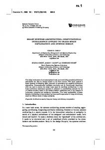
A. Training Time In ELM, as shown in Fig. 1, the training time is not affected by the small changes in the number of hidden nodes. The small random variations are due to processor variability. The fastest activation function was sine, followed by sigmoidal, then the radial basis, then hard limit, and then the triangular basis function. Moreover more training data results in more training time.
IMPLEMENTATION
Mainly, the methodology was implemented to provide comparable data. The input data were taken from Dr. Eren’s study, from which the multiple regression model is taken [5]. The same data set is inputted to ELM and RBF. A. Computer Codes Developed by Dr. Huang, a MATLAB function code is used to process data using ELM. To avoid variations due to random initializations, the code was run in a loop one thousand times and then an average is taken. ELM parameters are changed and compared to find the best combination. Parameters changed are the number of hidden neurons, activation function, and the percentage of training data. Regarding RBF, a MATLAB built in function (newrb) is used to process the data. Target training accuracy and percentage of training data are changed to find the best combination.
Figure 1. ELM training time
RBF requires more training time than ELM does. It requires more training time with lowering the target training RMSE. The spread effect on time is random. Furthermore, similar to ELM, more training data yields more time. Spread does not affect training times. The data for RBF are shown in Table II.
B. Input and Output Seven input drilling parameters were used in the study. These are depth, bit weight, rotary speed, tooth wear, Reynolds number function, ECD and pore gradient. The input data were chosen because they are the ones used in
34 32
TABLE II.
RBF TRAINING TIME
Set spread = 20 Target training RMSE(ft/hr)
Training Time (s)
70
0.1404
80
0.1404 Set spread = 30
Target training RMSE (ft/hr)
Training Time (s)
70
0.1248
80
0.1404
a
Set spread = 40 Target training RMSE (ft/hr)
Training Time (s)
70
0.1716
80
0.1560 Set spread = 50 Target training RMSE (ft/hr)
Training Time (s)
70
0.1716
80
0.1560
b Figure 2. ELM Training Accuracy, a) RMSE, b)SD
Set spread = 100 Target training RMSE (ft/hr)
RBF training accuracy is set to be either RMSE = 80 ft/hr or RMSE = 70 ft/hr. However the choice affects the time and accuracy of training and testing.
Training Time (s)
70
0.1872
80
0.1092
C. Testing Time Testing time for ELM seems random and unaffected by the number of hidden neurons. The sigmoid and sine functions gave the best results and hard limit, triangular basis, and radial basis gave the worst. Results are shown in Fig. 3.
B. Training Accuracy Using root mean square error (RMSE), standard deviation (SD), and absolute percent relative error (APRE), ELM gave relatively accurate training results. The accuracy gets better with increasing hidden neurons. Hard limit function provides the least accurate results. Other functions give very close RMSE values. The results can be deduced from Fig. 2 which shows the RMSE and SD of the data in ft/hr.
Figure 3. ELM testing time vs. No. of hidden neurons
35 33
RBF gave higher testing time than ELM. Testing time is not affected by the choice of goal training accuracy nor by the value of the spread, as in table III. TABLE III.
RBF TESTING TIME DATA Set spread = 20
Target training RMSE (ft/hr)
Testing Time (s)
70
0.0624
80
0.0936
Set spread = 30 Target training RMSE (ft/hr)
a Testing Time (s)
70
0.0936
80
0.0936
Set spread =40 Target training RMSE (ft/hr)
Testing Time (s)
70
0.0936
80
0.0468
Set spread=50 Target training RMSE (ft/hr)
Testing Time (s)
70
0.1092
80
0.0936
b
Set spread= 100 Target training RMSE (ft/hr)
Testing Time (s)
70
0.0624
80
0.1092
D. Testing Accuracy ELM's testing RMSE, SD, and APRE have minima at different number of hidden nodes at each activation function. Fig. 4 displays these minima.
c Figure 4. ELM Testing Accuracy, a) RMSE, b)SD, c)APRE
RBF testing was inaccurate when training target RMSE is 70ft/hr with a high value of spread. Testing accuracy values are very similar with spread change when RMSE = 80ft/hr. The results are shown in table IV.
36 34
TABLE IV.
RBF TESTING ACCURACY
TABLE V.
Set spread = 20 Target training RMSE (ft/hr)
Testing RMSE (ft/hr)
F-TEST, SIGMOIDAL, 80%, HN=10
F-Test Two-Sample for Variances Testing SD (ft/hr)
Variable 1
Testing APRE
Variable 2
Mean
170.2218
160.0496
70
85.7199
81.6799
36.11%
Variance
8021.917
5921.045
80
83.5978
40.7629
38.84%
Observations
96
96
df
95
95
Set spread = 30 Target training RMSE (ft/hr)
Testing RMSE (ft/hr)
Testing SD (ft/hr)
Testing APRE
70
145.8691
119.2764
67.76%
80
83.6105
40.7696
38.84%
F
1.354814
P(F