An alternative formulation for One-dimensional turbulence model (ODT), ... Hewson [5] used ODT model to turbulent reacting flows and demonstrated its ...
Application of an Eulerian One Dimensional Turbulence model to Simulation of Turbulent Jets Naveen K. Punati, James C. Sutherland
Department of Chemical Engineering, University of Utah, Salt Lake City, UT, USA
Abstract
An alternative formulation for One-dimensional turbulence model (ODT), an out-growth of LEM model, a method for stochastic simulation of turbulent �ows is proposed and applied for non-reacting jets. The formulation proposed herein solves the governing equations in an Eulerian frame of reference, rather than a Lagrangian frame as is traditionally done. Furthermore, equations for conserved variables, rather than primitive variables, are solved. After discussing the primary di�erences between the present formulation and prior formulations, we compare predictions of the model to data from a non- reacting propane-air jet. Ensemble averages for velocity and mixture fraction from multiple realizations of the �ow �eld are compared with experimental data. The predictions of the proposed approach for both temporal and spatial formulation shows good agreement with experimental data.
1 Introduction Turbulence is, inherently, three dimensional. The vortex stretching that causes the cascade of energy from large to small scales is not present in the Navier�Stokes equations in fewer than three dimensions. The One-Dimensional Turbulence (ODT) model developed by Kerstein, is formulated on a one-dimensional (1D) spatial domain simulates turbulent �ows to avoid the expense of computations in three dimensions by introducing a model for the nonlinear advective terms that drive turbulence through vortex stretching [1].
The ODT model has been successfully applied to sta-
tionary and decaying homogeneous turbulence, shear �ow, and various buoyant strati�ed �ows by evolving a single velocity component without accounting for interactions among velocity components [1]. ODT is an outgrowth of the Linear Eddy Model (LEM) developed by Kerstein [2]. LEM is a modeling strategy of maintaining a distinction between turbulent stirring and molecular di�usion on a 1D domain.
ODT generalizes LEM by using ideas from mixing length theory to allow the
scalar �elds to self-consistently determine the rate of turbulent mixing in the model, di�usive mixing is also explicitly represented on the small length scales. Hence turbulent advection and physical di�usion are algorithmically distinct processes within the ODT model. ODT model is capable of reproducing the turbulent cascade process, transferring �uctuations to successively smaller scales. Pressure-scrambling e�ects are incorporated in to the model by introducing a vector velocity �eld whose three components exchange energy in a manner that emulates pressure velocity interactions and successfully applied to free shear �ows by Ashurst [3]. Ashurst [4] generalized ODT to incorporate the kinematic and dynamical e�ects of density variations, examined performance of the model and the underlying physics of variable-density turbulence with reference to the measured structure and growth rate of variable-density planar mixing layers. Hewson [5] used ODT model to turbulent reacting �ows and demonstrated its capability to reproduce di�erential di�usion e�ects by studying the conditional means and �uctuations of temperature
1
and the species mass fractions.
Hewson and Kerstein [6] applied ODT model to study local ex-
tinction and reignition phenomena in non-premixed turbulent jet �ames. Echekki [7] discussed the di�erential di�usion e�ects in the near �ow region by applying ODT model to simulate turbulent di�usion �ames. By using ODT-based closure approach to predict scalar statistics to couple with the Reynolds-averaged Navier�Stokes (RANS), Ranganath [8] predicted the extinction and reignition in piloted methane�air jet di�usion �ames. ODT model is also used as a subgrid scale modeling technique for LES [9]. In the present paper we discuss the derivation of governing equations solved as part of ODT model in an Eulerian reference frame for temporal and spatial formulation, how the solution variables instead of primitive variables are solved, how the new approach enforces momentum conservation implicitly and calculation of kernel coe�cients from energy conservation principle. The discussion will be followed by code validation study.
2 Model Formulation In ODT we restrict the computational domain to a one-dimensional line of sight. For the present work we consider a domain aligned with the
x-direction.
The �elds de�ned on the one-dimensional
domain evolve by two mechanisms: molecular evolution and a stochastic process representing advection. For temporal �ows (T-�ows), each ODT realization represents a time history of the transverse pro�les of velocities, and/or time histories of scalar pro�les. For spatially developing �ows (S-�ows), ODT generates realizations parametrized by
(x; y)
instead of
(x; t),
where
y
is the streamwise coor-
dinate.
2.1 T-�ows The integral form of governing equations for conservation of mass,momentum, and energy along one-dimensional domain aligned with
ˆ
∂ρ dV V (t) ∂t ˆ ∂ρux dV V (t) ∂t ˆ ∂ρuy dV V (t) ∂t ˆ ∂ρYi dV V (t) ∂t ˆ ∂ρe0 dV V (t) ∂t where
ux , uy ,
and
usx
x-direction
may be written as
ˆ = −
ρ (ux − usx ) ax ds,
(1)
S(t)
ˆ
ˆ
= −
[ρux (ux − usx ) ax + τxx ax + pax ] dS + ρgx dV, V (t) ˆ ˆ = − [ρuy (ux − usx ) ax + τyx ax ] dS + ρgy dV, S(t) V (t) ˆ ˆ = − [ρYi (ux − usx ) ax + jix ax ] dS + Si dV, S(t) V (t) ˆ = − [ρe0 (ux − usx ) ax + qx ax + τxx ux ax + P ux ax ] dS,
(2)
S(t)
(3)
(4)
(5)
S(t) are the lateral, streamwise, control volume surface velocities respectively.
If the surfaces move with the same velocity as
ux , usx = ux ,
then the above governing equations
reduce to a Lagrangian formulation. Existing ODT implementations solve the governing equations in Lagrangian form. In the traditional approach the assumption
usx = ux
is equivalent to imposing
constant density, and mass conservation is enforced by modifying control volume sizes. The
y -momentum equation is solved in ODT to approximate local shear stress.
The shear stress,
in turn, a�ects the model for turbulence by in�uencing the rate at which model �eddies� occur.
2
In the current approach we set
usx = 0,
leading to an Eulerian formulation where the control
volumes are �xed in space and time. The advection mechanism represented by the stochastic process in ODT de�nes eddy motions based on variations in streamwise velocity otherwise to say the shear in streamwise direction, so even though the domain is represented in 1-D
y−momentum
equation
is also solved. Setting
usx = 0,
we arrive at the governing equations for the Eulerian form of the ODT model
proposed here,
∂ρ ∂t ∂ρux ∂t ∂ρuy ∂t ∂ρYi ∂t ∂ρe0 ∂t P The temperature
T
∂ρux , ∂x ∂ρux ux ∂P ∂ − − − (τxx ) , ∂x ∂x ∂x ∂ρuy ux ∂ − − (τxy ) , ∂x ∂x ∂ρYi ux ∂ − − (jix ) , ∂x ∂x ∂ρe0 ux ∂ ∂ ∂ − − (qx ) − (τxx ux ) − (P ux ) , ∂x ∂x ∂x ∂x ρRT . M
= −
(6)
=
(7)
= = = =
(8) (9) (10) (11)
is calculated from total internal energy and is subsequently used in the equation
of state (11) to �nd the pressure.
De�ning the constitutive relationships for
τxx ,τxy , jix
and
qx
completes the formulation.
2.2 S-�ows Occasionally we want to represent a spatially evolving �ow (S-�ow). Equations (6)-(10) are best suited for temporally evolving �ows (T-�ows). The equations derived for T-�ows are readily transformed to S-�ows by applying the chain rule,
∂φ ∂t
=
∂φ ∂y ∂y ∂t and noting that
uy ≡
∂y ∂t . Using this, the
governing equations for S-�ows represented as
∂ρ ∂y ∂ρux ∂y ∂ρuy ∂y ∂ρYi ∂y ∂ρe0 ∂y
1 ∂ρux , uy ∂x � � 1 ∂ρux ux ∂P ∂ − + + (τxx ) , uy ∂x ∂x ∂x � � 1 ∂ρuy ux ∂ − + (τxy ) , uy ∂x ∂x � � 1 ∂ρYi ux ∂ − + (jix ) , uy ∂x ∂x � � 1 ∂ρe0 ux ∂ ∂ ∂ − + (qx ) + (τxx ux ) + (P ux ) . uy ∂x ∂x ∂x ∂x
= −
(12)
=
(13)
= = =
(14)
(15)
(16)
2.3 Stochastic simulation method The stochastic process used to represent the e�ect of turbulence, propsed by Kerstein [3], consists of a sequence of events each of which involves an instantaneous transformation of the velocity and
3
scalar �elds. These events may be interpreted as the model analogue of individual turbulent eddies which are referred to as �eddy events� or simply �eddies�. Each eddy event is characterized by three properties: a length scale, a time scale, and a measure of kinetic energy, and a key physical input to the model is a postulated relationship among these quantities. The advection submodel is speci�ed by de�ning the mathematical operations performed during an eddy event and by formulating the rules that govern the random selection of events.
Because advection is implemented as an event
sequence rather than a continuous process, the velocity �eld does not directly prescribe the �uid motions. Motions and velocities are nevertheless closely linked through the dynamics embodied in the event selection rules. An eddy event consists of two mathematical operations. One is a measurepreserving map representing the �uid motions associated with a notional turbulent eddy(triplet mapping).
The other is a modi�cation of the velocity pro�les(kernel transformation) in order to
implement energy transfers prescribed by the dynamical rules.
These operations are represented
symbolically as
(ρu)i [x] = (ρu)i [f (x)] + ci K(x) According to this representation, �uid at location
f (x)
is moved to location
(17)
x
by the mapping
operation, which is the model analogue of the advection operator of the Navier-Stokes equations, is applied to all solution variables. The additive term
ci K(x),
a�ecting only the velocity components,
represents velocity changes due to pressure gradients or body forces and in vector formulation capture pressure-induced energy redistribution among velocity components.
2.3.1 Triplet map The functional form chosen for
f (x),
triplet map, is the simplest of a class of mappings that
satisfy the physical requirements of measure preservation, continuity and scale locality over the eddy interval can be represented in the following form
x0 ≤ x ≤ x0 + 13 l 3 (x − x0 ) 2l − 3 (x − x0 ) x0 + 13 l ≤ x ≤ x0 + 23 l . f (x) ≡ x0 + 3 (x − x0 ) − 2l x0 + 23 l ≤ x ≤ x0 + l This mapping takes a line segment
[x0 , x0 + l]
(18)
shrinks it to a third of its original length, and
then places three copies on the original domain. The middle copy is reversed, which ensures that property �elds remain continuous and introduces the rotational folding e�ect of turbulent eddy motion. Property �elds outside the size-l segment are una�ected.
2.3.2 Kernel Transformation K(x) is conveniently de�ned as K(x) = x−f (x) is continuous and integrates to zero over the eddy interval. The amplitudes ci are chosen to transfer the amount of kinetic energy speci�ed 00 by the model. Change in i-component momentum (ρu)i can be represented as, The kernel
00
0
(ρu)i = (ρu)i + ci K(x), where
0
(ρu)i
(19)
represents triplet mapped momentum �eld. Solving for momentum deterministically
instead of velocities along with continuity equation enforces the momentum conservation implicitly avoiding the computation of extra kernel to account for variable density e�ects.
4
An eddy event causes the kinetic energy of velocity component
1 2
= ∆Ei
ˆ h
(20)
(21)
can be represented as
4Ei =
� 1� 2 ci A + 2ci Bi , 2
(22)
´ (ρu)0i K Bi = dx. For a three velocity component system conservation of ρ0 kinetic energy, 4Ei = 0, imposes only one constraint on (22) in calculating the amplitudes of ci . Further modeling to determine the three amplitudes is based on the following observation. ci for given i can be chosen so as to add an arbitrarily large amount of kinetic energy to component i,
where
A=
´
to change by an amount
i 00 0 00 0 (ρui ) ui − (ρu)i ui dx # 0 0 ˆ " 00 00 (ρu) (ρu)i (ρu)i 1 i (ρu)i − dx 2 ρ0 ρ0
4Ei =
From (19) and (21),
i
K2 0 dx and ρP
but the maximum amount that can be removed is a �nite value, which is evaluated by maximizing the kinetic energy change with respect to
ci
d(4Ei ) 1 = [2ci A + 2Bi ], dci 2 so that
ci = − De�ne
Qi
Bi . A
(23)
as the maximum energy that can be removed from velocity component
Qi = −
i,
Bi2 2A
(24)
Motivated by the phenomenological interpretation of pressure scrambling as a tendency to restore isotropy, the amplitudes are further constrained by requiring invariance under exchange of indices. The kinetic energy changes imposed on the velocity components must be of the form,
4Ei where
α
is a model parameter and
The value
α=1
� � 1 = α −Qi + (Qj + Qk ) , 2
{i, j, k}
is any permutation of the component indices
(25)
{1, 2, 3}.
maximizes the inter-component transfer.
From (22), (24) and (25), expressions for amplitudes of
ci
ci
v u� �2 Bi u Bi α = − (1 − α) + ±t A A 2
can be formulated as
! Bk2 + . A A
Bj2
(26)
2.3.3 Eddy rate distribution The physical model, developed by Ashurst [4], used to decide whether to accept a selected eddy is described in this section. The quantity
ρl3 l τ is interpreted as an eddy velocity and τ 2 is interpreted as 5
a measure of the energy of eddy motion. To determine eddy turn over time
τ
this energy is equated
to an appropriate measure of the eddy energy based on the current �ow state, which is, available energy of the
i=2
velocity component upon completion of eddy implementation, minus an energy
penalty that re�ects viscous dissipation e�ects.
� �2 l ∼ τ where
C
2 νavg (1 − α)Q2 + α2 (Q1 + Q3 ) −Z 2 . ρavg l l
(27)
is an adjustable parameter that controls the overall event frequency and
penalty coe�cient. disallowed.
Z
is a viscous
If the eddy energy cannot overcome the viscous dissipation e�ects eddy is
The energy penalty introduces a threshold Reynolds number that must be exceeded
for eddy turnover to be allowable. Eddy rate distribution governing the occurrence of eddy events during simulated realizations is de�ned from scaling analysis and 27 as
λ = =
C , l2 τs � � 2 νavg C (1 − α) Q2 + α (Q1 + Q3 ) − Z . l3 ρavg l l2
(28)
(29)
2.3.4 Large eddy suppression The eddy selection procedure can occasionally allow the occurrence of large unphysical eddies. This is more commonly seen in the case of free shear �ows than wall bounded �ows.
A method for
suppressing these highly energetic eddies, developed by Ashurst [4], is implemented into the ODT formulation.
This procedure termed as the scale-reduction method involves auxiliary eddy-rate
computations for each of three equal sub-intervals of the eddy interval[x0 , x0
� � λ is evaluated as if the eddy interval were x0 + (j − 1) 3l , x0 + j 3l ,
+ l]. In other words, for j = 1, 2, and 3, respectively.
If any of these three candidate eddies are disallowed due to dominance of the viscous penalty, then the acceptance probability is set to zero. Otherwise it is unchanged from its value computed for the complete eddy interval
[x0 , x0 + l].
In the implementation of this method, the viscous penalty
employed in the sub-interval computations is based on the size of the complete eddy interval, not the sub-interval size.
2.3.5 Eddy selection For each eddy event, eddy length(l) and location(x0 ) selected from randomly generated numbers and �ow properties. From scaling analysis eddy length and shear stress value eddy starting location will be calculated. For the selected
x0 , l ,
eddy rate distribution will be calculated using the procedure
outlined so far. Based on the probability density functions de�ned for of
x0 , l
and
λ,
probability
will be calculated using
probability = where
λdt f (x0 )g(l)
(30)
dt is integration step size and f (x0 ), g(l) are probability density functions for x0 , l respectively
de�ned as
6
f (x0 ) = g(l) = where
Lp , eddymax ,
and
eddymin
ceddy exp l2
�
−2Lp l
� ,
1 , eddymax − eddymin
are the most probable eddy length, maximum and minimum eddy
size respectively. If the probability calculated from (30) is greater than a randomly selected number on the interval
[0, 1]
then eddy will be accepted.
3 Results & Discussion 3.1 Non-reacting Propane-Air jet In this work, the radial and axial pro�les of the mean streamwise velocity and mixture fraction that are predicted by the model (after ensemble averaging) are compared with those of the experiment. The non-reacting propane jet measurements taken as a part of the International-Workshop on Measurement and Computation of Turbulent Non-premixed �ames [10] are used for this validation study.
3.1.1 Initial Conditions The initial conditions used for simulating non-reacting propane jet are given in Table 1. The velocity
Table 1: Initial conditions. Reynolds number
68000
Inner Diameter
0.0052 m
Outer Diameter
0.0090 m
Propane Jet velocity
53 m/s
Propane Jet Temperature
294 K
Co-�ow air velocity
9.2 m/s
Co-�ow Air Temperature
294 K
and scalars pro�les at the inlet are de�ned by
� � �� � � � ��� A x − L1 1 x − L2 ϕ(x) = 1 + tanh 1− 1 + tanh , 2 w 2 w where
A
is the amplitude of the change
w
is the width of the transition and
midpoints of the transition. This is illustrated in Figure 1.
7
L1
and
L2
are the
Figure 1: Schematic of tanh pro�le used to specify scalar and mean velocity pro�les
3.1.2 T-�ows An indirect approach has been adopted to compare the temporal �ows simulation results with experimental data. Based on the average streamwise velocity at each time step an ordinary di�erential equation is solved to determine the axial location of ODT line,
dy =u ¯y , dt where
u ¯y
is a suitable average of the
y -velocity.
The variation in the mean velocity along the jet centerline is compared with experimental data
4
in Figure 2.
The radial pro�les of the mean axial velocity at
4, 15, 30, 50
are compared with experimental data in Figure 3.
di�erent axial locations,
y/D =
In this work, the experimental
data obtained by seeding the jet stream are used for the comparison with ODT prediction. Good agreement between the ODT results and the experiments is seen at all axial locations except at
y/D = 50.
The spreading rate predicted by the model matches with the experimental data at all
axial locations, but the over prediction in the velocity can be seen at
y/D = 50.
is also predicted by mean centerline velocity decay in Figure 2.
70 Expt ODT
Mean Centerline Velocity
60
50
40
30
20
10
0
0
10
20
30
40
50
60
70
80
90
x/D
Figure 2: Centerline pro�le of mean streamwise velocity
8
The same behavior
50 Expt ODT
60
Mean Streamwise Velocity
Mean Streamwise Velocity
70
50 40 30 y/D = 4 20 10 0 −6
−4
−2
0 x/D
2
4
20
y/D = 15
10
−4
−2
0 x/D
2
4
6
25 Expt ODT
Mean Streamwise Velocity
Mean Streamwise Velocity
30 25 20 y/D = 30
15 10 5 −6
30
0 −6
6
Expt ODT
40
−4
−2
0 x/D
2
4
Expt ODT
20
10
5 −6
6
y/D = 50
15
−4
−2
0 x/D
2
4
6
Figure 3: Mean radial pro�les of streamwise velocity at di�erent axial locations
The variation in the mean mixture fraction along the jet centerline is compared with experimental data in Figure 4. As seen from the �gure, the mean centerline mixture fraction remains constant for few jet diameters downstream of the jet exit before it starts to decay. This region is called the potential core of the jet. In the potential core region, the e�ects of viscous shear and di�usion are not very signi�cant and hence the mixture fraction remains unchanged from its nozzle exit value. Beyond this region, the mean mixture fraction decreases rapidly as co-�owing air is entrained by the jet. The decay of the centerline mixture fraction predicted by the ODT model is rapid between
10 − 25
jet diameters and slows down after that.
The radial pro�les of the mean mixture fraction at four di�erent axial locations are also compared with experimental data in Figure 5. The pro�les at
y/D = 4, 15, 30
and
50
show good agreement
between the simulations and the experiment although a slightly higher value of the mixture fraction towards the centerline is predicted by the ODT model at
y/D = 50.
As seen in Figure 4, this region
was over-predicted by the ODT model.
1 Expt ODT
Mean Centerline Mixture Fraction
0.9 0.8 0.7 0.6 0.5 0.4 0.3 0.2 0.1 0
0
10
20
30
40 x/D
50
60
70
80
Figure 4: Centerline pro�le of mean mixture fraction
9
0.6
1 0.8
Mean Mixture Fraction
Mean Mixture Fraction
Expt ODT
0.6 0.4
y/D = 4
0.2 0 −6
−4
−2
0 x/D
2
4
Expt ODT
0.5 0.4 0.3 y/D = 15
0.2 0.1 0 −6
6
−4
−2
0 x/D
2
4
6
0.4 Mean Mixture Fraction
Mean Mixture Fraction
Expt ODT
0.3
0.2 y/D = 30 0.1
0 −6
−4
−2
0 x/D
2
4
Expt ODT
0.25 0.2 0.15
y/D = 50 0.1 0.05 0 −6
6
−4
−2
0 x/D
2
4
6
Figure 5: Mean radial pro�les of mixture fraction at di�erent axial locations
3.1.3 S-�ows Figure 6 shows the comparison between the experimental data and model prediction for centerline
4
velocity decay.
The radial pro�les of the mean axial velocity at
= 4, 15, 30, 50
are compared with experimental data in Figure 7.
reasonable agreement with data for
y/D ≤ 15,
di�erent axial locations,
y/D
Though the prediction is in
signi�cant di�erence is observed for
y/D ≥ 25 which
is also clearly evident in center line velocity decay in Figure 6. The spreading rate predicted by the model matches with the experimental data at all axial locations, but the over prediction in the velocity can be seen for
y/D ≥ 30. 70 Expt ODT
Mean Centerline Velocity
60
50
40
30
20
10
0
0
10
20
30
40
50
60
70
80
90
x/D
Figure 6: Centerline pro�le of mean streamwise velocity
10
50 Expt ODT
Mean Streamwise Velocity
Mean Streamwise Velocity
80
60 y/D = 4 40
20
0 −6
−4
−2
0 x/D
2
4
y/D = 15
20 10
−4
−2
0 x/D
2
4
6
30 Expt ODT
30
Mean Streamwise Velocity
Mean Streamwise Velocity
30
0 −6
6
35
25 y/D = 30 20 15 10 5 −6
Expt ODT
40
−4
−2
0 x/D
2
4
Expt ODT
25 20
y/D = 50
15 10 5 0 −6
6
−4
−2
0 x/D
2
4
6
Figure 7: Mean radial pro�les of streamwise velocity at di�erent axial locations
The variation in the mean mixture fraction along the jet centerline predicted by the model shows signi�cant deviation from the experimental data in Figure 8. The decay is over-predicted for
y/D < 15
and under-predicted downstream. Figure 9 shows the comparison between radial pro�les
predicted by the model and experimental data at di�erent axial locations. High Spreading rate and higher mixture fraction values are predicted by the model in the region
y/D ≥ 15
evident from Figure 8 where slow decay is observed in the same region.
1 Expt ODT
Mean Centerline Mixture Fraction
0.9 0.8 0.7 0.6 0.5 0.4 0.3 0.2 0.1 0
0
10
20
30
40
50
60
70
x/D
Figure 8: Centerline pro�le of mean mixture fraction
11
which is also
0.6 Expt ODT
0.8 0.6
Mean Mixture Fraction
Mean Mixture Fraction
1
y/D = 4
0.4 0.2 0 −6
−4
−2
0 x/D
2
4
0.4
y/D = 15 0.3 0.2 0.1 −4
−2
0 x/D
2
4
6
0.5 Expt ODT
Mean Mixture Fraction
Mean Mixture Fraction
0.4
0 −6
6
Expt ODT
0.5
0.3 y/D = 30 0.2
0.1
0 −6
−4
−2
0 x/D
2
4
y/D = 15
0.3 0.2 0.1 0 −6
6
Expt ODT
0.4
−4
−2
0 x/D
2
4
6
Figure 9: Mean radial pro�les of mixture fraction at di�erent axial locations
4 Conclusions The ODT model of Kerstein [1] was reformulated using an Eulerian approach. Simulation results from both temporal and spatial formulation are compared with experimental data of a spatially developing non-reacting propane jet.
The validation study has shown that the ODT formula-
tion can provide qualitative agreement with experimental data.
Entrainment and mixing e�ects
are represented better by the temporal formulation than for spatial formulation. Further adjustment/optimization of model parameters, as well as modifying initial conditions and changing mesh resolution may result in better agreement between model prediction and experimental data. The approach proposed herein (Eulerian) is quite di�erent from the traditional ODT approaches in the following respects:
•
It solves the momentum equation in the tuations in the
x-direction.
x-direction
and directly incorporates pressure �uc-
The implementation described herein treats this in a fully com-
pressible manner.
•
It uses a static mesh whereas other formulations for variable density �ow using ODT rely on a Lagrangian mesh where cell volumes change to maintain zero advective �uxes through cell boundaries.
•
The eddy events are implemented di�erently than traditional ODT approaches.
We apply
(18) directly, interpolating values as needed. In the traditional approach, a discrete analog of (18) is used, where Lagrangian volumes are relocated in space. Thus, while our mesh is una�ected by triplet mapping, traditional ODT approaches must remesh when a triplet map occurs.
•
We solve the governing equations for conserved quantities
ρux , ρuy , ρ, ρe0 , ρYi ,
whereas
previous formulations solve the primitive equations. Application of triplet maps to the primitive variables requires additional kernel transformations to ensure conservation; we apply the
12
triplet map to the conserved variables and thus do not require additional kernel transformations. The only kernel transformation required in this formulation is on the momentum to guarantee conservation of kinetic energy. In the event that a nonuniform mesh is employed, an additional kernel transformation is required to maintain conservation. Both temporal and spatial formulations are directly applicable for reacting �ows as well. Comparison with turbulent reacting jet �ames (Sandia �ames D and E) is currently underway. Future work will focus on evaluating ODT against DNS data to determine if statistics from DNS can be reasonably represented by ODT so that ODT can form the basis for subgrid modeling of turbulent reacting �ow.
5 References 1. Kerstein, A. R., J. Fluid Mech 392:277 (1999). 2. Kerstein, A. R., J. Fluid Mech 216:411 (1990). 3. Kerstein, A. R., Ashurst, Wm. T., Wunch, S., Nilsen, V., J. Fluid Mech 447:85 (2001). 4. Ashurst, Wm. T., Kerstein, A. R., Phys. Fluids 17:26 (2005). 5. Hewson, J. C., Kerstein, A. R., Combust. Theo. Modelling 5:669 (2001). 6. Hewson, J. C., Kerstein, A. R., Combust. Sci. and Tech 174:35 (2002). 7. Echekki, T., Kerstein, A. R., Dreeben, T. D., Combust. Flame 125:1083 (2001). 8. Ranganath, B., Echekki, T., Combust. Flame 154:23 (2008). 9. McDermott, R. J. (2001). Ph.D. thesis, University of Utah. 10. International workshop on measurement and computation of turbulent nonpremixed �ames. http://public.ca.sandia.gov/TNF/abstract.html.
13