Application of an Unstructured Grid-Based Water Quality Model ... - MDPI

Journal of

Marine Science and Engineering Article

Application of an Unstructured Grid-Based Water Quality Model to Chesapeake Bay and Its Adjacent Coastal Ocean Meng Xia * and Long Jiang Department of Natural Sciences, University of Maryland Eastern Shore, Princess Anne, MD 21853, USA; [email protected] * Correspondence: [email protected]; Tel.: +1-410-621-3551 Academic Editor: Richard P. Signell Received: 11 July 2016; Accepted: 18 August 2016; Published: 1 September 2016

Abstract: To provide insightful information on water quality management, it is crucial to improve the understanding of the complex biogeochemical cycles of Chesapeake Bay (CB), so a three-dimensional unstructured grid-based water quality model (ICM based on the finite-volume coastal ocean model (FVCOM)) was configured for CB. To fully accommodate the CB study, the water quality simulations were evaluated by using different horizontal and vertical model resolutions, various wind sources and other hydrodynamic and boundary settings. It was found that sufficient horizontal and vertical resolution favored simulating material transport efficiently and that winds from North American Regional Reanalysis (NARR) generated stronger mixing and higher model skill for dissolved oxygen simulation relative to observed winds. Additionally, simulated turbulent mixing was more influential on water quality dynamics than that of bottom friction: the former considerably influenced the summer oxygen ventilation and new primary production, while the latter was found to have little effect on the vertical oxygen exchange. Finally, uncertainties in riverine loading led to larger deviation in nutrient and phytoplankton simulation than that of benthic flux, open boundary loading and predation. Considering these factors, the model showed reasonable skill in simulating water quality dynamics in a 10-year (2003–2012) period and captured the seasonal chlorophyll-a distribution patterns. Overall, this coupled modeling system could be utilized to analyze the spatiotemporal variation of water quality dynamics and to predict their key biophysical drivers in the future. Keywords: FVCOM-ICM; Chesapeake Bay; water quality; nutrient; phytoplankton; dissolved oxygen

1. Introduction As the largest and most biologically-diverse coastal plain estuary in North America [1], Chesapeake Bay (CB) is highly influenced by its vast watershed with a land-to-water ratio of 14.3 [2]. Following the population growth, industrial and agricultural development, CB has undergone severe eutrophication with symptoms of excessive nutrient loading, nuisance algal blooms, extensive summer hypoxia and declined seagrass coverage since the mid-1900s [3,4]. Typically, the overloading of cultural nutrients into CB directly drives its water quality deterioration, including bottom hypoxia/anoxia, overwhelming phytoplankton growth and diminished water clarity [2]. Biogeochemical cycles in CB and similar water bodies have been investigated using field investigation [5–7], retrospective long-term data analysis [8,9], remote sensing images [10], and numerical simulations [11,12]. Intra-seasonal and inter-annual observed data can effectively detect the dominant environmental factors driving water quality variations, but is usually limited by sparse spatiotemporal resolution [13]. Satellite imagery provides synoptic surface phytoplankton and suspended material distribution while it is incapable of exhibiting vertical variation [10]. Statistical

J. Mar. Sci. Eng. 2016, 4, 52; doi:10.3390/jmse4030052

www.mdpi.com/journal/jmse

J. Mar. Sci. Eng. 2016, 4, 52

2 of 23

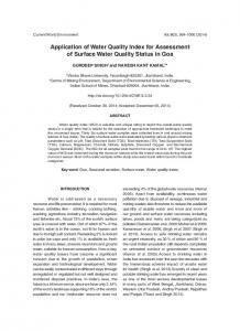
empirical models and simplified oxygen models omitting nutrient cycles have been developed as substitutes for specific research goals, but it is impossible to reproduce the detailed internal spatiotemporal water quality variation and comparatively evaluate biophysical drivers [14]. In contrast, the three-dimensional physical-biogeochemical model could better resolve the biophysical interactions between circulation and water quality kinetics [11,12] and facilitate mechanistic analysis of internal water-column dynamics [15–17], making it an ideal tool to investigate nutrient dynamics and algal variability in eutrophic estuaries [18], synoptically assess estuarine biophysical processes and project future scenarios [19,20]. However, there exist several challenges and limitations in developing and applying sophisticated biophysical models [20]. For example, low-resolution models have difficulty following the coastline or investigating the tributary-estuary exchange very well. Unstructured grid models have the advantage of flexibility reaching fine resolution at areas of interest (e.g., nearshore, sills, deep channels and fronts) over the structured grid models [21]. Other key challenges and sources of uncertainty in configuring biophysical models lay in meteorological forcing, hydrodynamic simulation and nutrient loading [20]. For example, turbulent mixing and bottom roughness are key factors for the bay circulation [22], while their effects on the water quality dynamics are less investigated. In addition, uncertainties and errors originating from these processes have been poorly compared and discussed in any biophysical model application, and these limitations could be magnified when modeling a biologically-diverse estuary (e.g., CB) and cause biases when interpreting the model simulations and providing management suggestions [12,23]. Since high resolution would potentially benefit the water quality simulation, a three-dimensional biophysical model was configured for CB, its tributaries and adjacent coastal ocean based on the unstructured grid modeling framework FVCOM-ICM [24], which comprises the hydrodynamic model, the finite-volume coastal ocean model (FVCOM) and a water quality component, the modified Corps of Engineers Integrated Compartment Water Quality Model (FVCOM-ICM, [24]). During the model development, we tried to achieve a comprehensive understanding of various uncertainties for the model development and answer the following questions: (1) how will increased model resolution improve the simulation of water quality variables; (2) how sensitive is the model to different wind sources; and (3) what is the most significant physical and biological sources of uncertainty in our model? Sections 2 and 3 introduce the model frame and sensitivity experiments; model calibration results are depicted in Section 4; Section 5 lists the major conclusions. 2. Material and Methods 2.1. Study Site CB, located adjacent to the Mid-Atlantic Bight on the east coast of United States (Figure 1), is a partially-mixed drowned river valley with a residence time of 90–300 days depending on the river flux [2,25]. A deep channel in the middle and shoals on both flanks (Figure 1 [2]) characterize the main stem of this large estuary with an area of 11,600 km2 (323 km long, 48 km wide and 6.5 m deep on average), where the salinity typically ranges from 0–30 from the northern to the southern end. A two-layer estuarine circulation is subject to variation in river flux, local/remote winds, semidiurnal tides and other forces [26,27]. Receiving 337.3 kt/year (kt = thousand tons) nitrogen and 23.7 kt/year phosphorus inputs by 2010 [28], CB generates 2–12 km3 bottom hypoxic waters every summer [29] and witnesses frequent occurrence of harmful algal blooms [30], which threatens the bay’s living resources and ecological service to its recreational and commercial users.

J. Mar. Sci. Eng. 2016, 4, 52 J. Mar. Sci. Eng. 2016, 4, 52   

3 of 23

3 of 23 

  Figure 1. Model grid and bathymetry of of  Chesapeake Bay (CB) and its its  adjacent coastal ocean with river Figure  1.  Model  grid  and  bathymetry  Chesapeake  Bay  (CB)  and  adjacent  coastal  ocean  with  nodes, data sites and three transects. The bottom right panels are the zoom-in of the boxed area from river nodes, data sites and three transects. The bottom right panels are the zoom‐in of the boxed area  two sets of grids generated for sensitivity experiments on spatial resolution. Sus, Susquehanna River; from two sets of grids generated for sensitivity experiments on spatial resolution. Sus, Susquehanna  Ptp, Patapsco Che,River;  Chester River; Pat, River;  Patuxent River; Cho, River;  Choptank River; Pot, Potomac River; River;  Ptp,  River; Patapsco  Che,  Chester  Pat,  Patuxent  Cho,  Choptank  River;  Pot,  Nan, Nanticoke River; Rap, Rappahannock River; Yor, York River; Jam, James River. Potomac River; Nan, Nanticoke River; Rap, Rappahannock River; Yor, York River; Jam, James River. 

2.2.2.2. Model Description  Model Description unstructured grid grid FVCOM-based FVCOM‐based  hydrodynamic hydrodynamic  model  the  water  AnAn  unstructured modelwas  wasused  usedto tosimulate  simulate the water level, temperature, salinity, circulation, eddy viscosity and other hydrodynamic information at an  level, temperature, salinity, circulation, eddy viscosity and other hydrodynamic information at an external  and  internal  time step step of of 33 ss and and 12 12 s,s, respectively respectively  [31].  existing  external and internal time [31]. This  Thiswork  workadopted  adoptedthis  this existing hydrodynamic model with the grid size ranging from 270 m–20.9 km (Figure 1). The major external  hydrodynamic model with the grid size ranging from 270 m–20.9 km (Figure 1). The major external forcing was comprised of daily river discharge, atmospheric forcing and open boundary conditions.  forcing was comprised of daily river discharge, atmospheric forcing and open boundary conditions. The hydrodynamic data sources, calibration and validation processes and the justification of model  The hydrodynamic data sources, calibration and validation processes and the justification of model settings could be retrieved in detail from [31].  settings could be retrieved in detail from [31]. The water quality kinetics, including nutrient cycles, sediment diagenesis and plankton growth,  The water quality kinetics, including nutrient cycles, sediment diagenesis and plankton growth, was  simulated  in  the  FVCOM‐based  water  quality  model  FVCOM‐ICM  [24].  Integrated  was simulated in the FVCOM-based water quality model FVCOM-ICM [24]. Integrated Compartment Compartment Model (ICM) was originally developed for the CB restoration and now works as part  Model (ICM) was originally developed for the CB restoration and now works as part of the predictive of the predictive model package CBEMP for the total maximum daily load plan [11,28]. A primary  model package CBEMP for theand  totalFVCOM‐ICM  maximum daily load plan [11,28]. A primary difference difference  between  CBEMP  is  our  use  of  the  unstructured  grid  and  the  between sigma  CBEMP and FVCOM-ICM is our use of the unstructured grid and the sigma coordinate to accommodate coordinate  to  accommodate  the  complex  bay  coastline and  bathymetry.  The mass  balance  of  state  thevariables in each control volume/cell [11] is solved as follows.  complex bay coastline and bathymetry. The mass balance of state variables in each control volume/cell [11] is solved as follows. n n

VC





C

y

y

 Qk Ck  Ak Dk  VS   (1)  ∂VC t = kn1 Q C + kn1 A D ∂C x + VS   (1) ∑ k k ∑ k k ∂x ∂t k =1 3 k =1 In Equation, V is the volume of a cell (m ), C is the concentration or biomass in the cell (mg/L), t  3/s), Ck  is the temporal coordinate (s), Qk is the flux across the interface with the k‐th neighbor cell (m In Equation, V is the volume of a cell (m3 ), C is the concentration or biomass in the cell (mg/L), is the concentration or biomass across the interface between two cells (mg/L), Ak is the interface area  t is the temporal coordinate (s), Qk is the flux across the interface with the k-th neighbor cell (m3 /s), 2/s), n is the number of neighbor cells, i.e., the  (m2), Dk is the diffusion coefficient at the interface (m Ck is the concentration or biomass across the interface between two cells (mg/L), Ak is the interface number of interfaces, x is the spatial coordinate (m) and S is the changing rate due to external loads  area (m2 ), Dk is the diffusion coefficient at the interface (m2 /s), n is the number of neighbor cells, i.e., and kinetic reaction in the cell (mg∙L−1∙s−1). To adapt to the sigma (σ) coordinate system, the transport  theof each state variable is modified as below [24].  number of interfaces, x is the spatial coordinate (m) and S is the changing rate due to external loads −1 −1 and kinetic the cellC (mg CD reaction Csystem, the transport  ·L  ·s ). To Cadapt to the sigma C (σ)  CuD in CvD 1 coordinate A H  A H  A H     ( ) ( ) ( )  DS   (2)  h v of each state variable is modified as belowh [24]. t

x

y



x

x

D 



∂CD ∂CuD ∂CvD ∂Cω ∂ ∂C ∂ ∂C 1 ∂ ∂C + + + = ( A H ) + ( Ah H ) + ( Av H ) + DS ∂t ∂x ∂y ∂σ ∂x h ∂x ∂y ∂y D ∂σ ∂σ

(2)

J. Mar. Sci. Eng. 2016, 4, 52

4 of 23

J. Mar. Sci. Eng. 2016, 4, 52   

4 of 23 

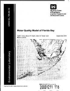
In the equation, D is total depth (H + ζ, m), where H is the mean water depth and ζ is the water In the equation, D is total depth (H + ζ, m), where H is the mean water depth and ζ is the water  elevation, Ah is the horizontal diffusivity (m22/s), Av is the vertical diffusivity (m2 2 /s), u, v and ω are elevation, Ah is the horizontal diffusivity (m /s), Av is the vertical diffusivity (m /s), u, v and ω are  velocity components (m/s) in the directions of x, y and σ, respectively, and S is the biogeochemical velocity components (m/s) in the directions of x, y and σ, respectively, and S is the biogeochemical  changing rate (mg·L−−11 ·s−1−1 ). changing rate (mg∙L ∙s ).  We simulated a total of 26 state variables in carbon, nitrogen, phosphorus, silicon and We simulated a total of 26 state variables in carbon, nitrogen, phosphorus, silicon and dissolved  dissolved oxygen (DO) cycles (Figure 2), including total suspended solids (TSS), cyanobacteria, oxygen  (DO)  cycles  (Figure  2),  including  total  suspended  solids  (TSS),  cyanobacteria,  diatoms,  diatoms, dinoflagellates, microzooplankton (20–200 µm), mesozooplankton (0.2–20 mm), ammonia dinoflagellates,  microzooplankton  (20–200  μm),  mesozooplankton  (0.2–20  mm),  ammonia  (NH4),  (NH4), nitrite and nitrate (NO23), phosphate (PO4), particulate inorganic phosphorus (PIP), nitrite  and  nitrate  (NO23),  phosphate  (PO4),  particulate  inorganic  phosphorus  (PIP),  labile/refractory dissolved/particulate organic carbon (LDOC, RDOC, LPOC, RPOC), labile/refractory labile/refractory  dissolved/particulate  organic  carbon  (LDOC,  RDOC,  LPOC,  RPOC),  dissolved/particulate organic nitrogenorganic  (LDON,nitrogen  RDON,(LDON,  LPON, RDON,  RPON), LPON,  labile/refractory labile/refractory  dissolved/particulate  RPON),  dissolved/particulate organic phosphorus (LDOP, RDOP, LPOP, RPOP), chemical oxygen demand labile/refractory dissolved/particulate organic phosphorus (LDOP, RDOP, LPOP, RPOP), chemical  (COD), DO and particulate/dissolved silica (PSi/DSi). The sub-models of sediment diagenesis [32] and oxygen demand (COD), DO and particulate/dissolved silica (PSi/DSi). The sub‐models of sediment  bivalve filtration [33] were turned on. ICM in CBEMP showed considerable model skills in representing diagenesis  [32]  and  bivalve  filtration  [33]  were  turned  on.  ICM  in  CBEMP  showed  considerable  the water quality variables forthe  decades [11], so variables  most of their model settings were model  skills  in  representing  water  quality  for  decades  [11],  so  and most parameters of  their  model  followed (Table 1). settings and parameters were followed (Table 1). 

  Figure 2. Schematic flow diagram of ICM set up for Chesapeake Bay. LDOC, RDOC, LPOC, RPOC,  Figure 2. Schematic flow diagram of ICM set up for Chesapeake Bay. LDOC, RDOC, LPOC, labile/refractory  dissolved/particulate  organic organic carbon;  LDON,  RDON,  LPON,  RPOC, labile/refractory dissolved/particulate carbon; LDON, RDON, LPON,RPON,  RPON, labile/refractory  dissolved/particulate  organic  nitrogen;  LDOP,  RDOP,  LPOP,  RPOP,  labile/refractory dissolved/particulate organic nitrogen; LDOP, RDOP, LPOP, RPOP, labile/refractory labile/refractory  dissolved/particulate  organic  phosphorus;  PSi/DSi,  particulate/dissolved  silica;  dissolved/particulate organic phosphorus; PSi/DSi, particulate/dissolved silica; COD, chemical COD, chemical oxygen demand; DO, dissolved oxygen; NO23, nitrite and nitrate; NH4, ammonia;  oxygen demand; DO, dissolved oxygen; NO23, nitrite and nitrate; NH4, ammonia; PO4, phosphate; PO4, phosphate; DIN, dissolved inorganic nitrogen.  DIN, dissolved inorganic nitrogen. Table 1. Key kinetic parameters used for the ICM for Chesapeake Bay. CHLA, chlorophyll = a.  Table 1. Key kinetic parameters used for the ICM for Chesapeake Bay. CHLA, chlorophyll = a.

Parameters  Parameters Settling velocity W (CYN, m/day)  Settling velocity W (CYN, m/day) Settling velocity W (DIA, m/day)  Settling velocity W (DIA, m/day) Settling velocity W (DINO, m/day)  Settling velocity W (DINO, m/day) −1)  Max photosynthetic rate P m (CYN, day Max photosynthetic rate Pm (CYN, day−1 ) − 1 −1 Max photosynthetic rate Pm (DIA, day ) Max photosynthetic rate P m (DIA, day )  Max photosynthetic rate Pm (DINO, day−1 ) Max photosynthetic rate P m (DINO, day−1)  C:CHLA ratio CChl (CYN) C:CHLA ratio CChl (CYN)  C:CHLA ratio CChl (DIA) C:CHLA ratio CChl (DIA)  C:CHLA ratio CChl (DINO) Half-saturation KH-DIN (CYN, mg/L) C:CHLA ratio CChl (DINO)  Half-saturation KH-DIN (DIA, mg/L) Half‐saturation K  (CYN, mg/L)  Half-saturation KH-DINH‐DIN (DINO, mg/L) Half‐saturation K H‐DIN  (DIA, mg/L)  Half-saturation KH-DIP (all, mg/L) Half-saturation KH-DSi (DIA, mg/L) Half‐saturation K H‐DIN  (DINO, mg/L)  Photosynthesis Topt (CYN, ◦ C) Half‐saturation K H‐DIP (all, mg/L)  Photosynthesis Topt (DIA, ◦ C) ◦ C) Half‐saturation K H‐DSi  (DIA, mg/L)  Photosynthesis Topt (DINO, Photosynthesis Topt (CYN, °C)  Photosynthesis Topt (DIA, °C)  Photosynthesis Topt (DINO, °C) 

Value

Literature Range  Literature Range 0–0.1 [11,14,34]  00.2  0–0.1 [11,14,34] 0–0.5 [11,14,21,34]  0.2 0–0.5 [11,14,21,34] 0.1  0–0.2 [21,34]  0.1 0–0.2 [21,34] 150  100–270 [11,14,34]  150 100–270 [11,14,34] 300 200–400 [11,14,21,34] 300  200–400 [11,14,21,34]  200 200–350 [21,34] 200  200–350 [21,34]  50 30–143 [11,14,34,35] 30–143 [11,14,34,35]  3750  30–143 [11,14,21,34,35] 30–143 [11,14,21,34,35]  5037  30–143 [21,34,35] 0.02 0.01–0.03 [11,14,34]  50  30–143 [21,34,35] 0.025 0.003–0.923 [11,14,21,34]   0.02  0.01–0.03 [11,14,34] 0.025 0.003–0.923 [21] 0.025  0.003–0.923 [11,14,21,34] 0.0025 0.001–0.195 [11,14,21,34]   0.03 0.01–0.05 [11,14,21,34] 0.025  0.003–0.923 [21]  25 22–30 [11,14,34]   0.0025  0.001–0.195 [11,14,21,34] 16 12–35 [11,14,21,34]   0.03  0.01–0.05 [11,14,21,34] 24 18–35 [21] 25  22–30 [11,14,34]  16  12–35 [11,14,21,34]  24  18–35 [21]  Value 0 

J. Mar. Sci. Eng. 2016, 4, 52

5 of 23

Table 1. Cont. Parameters

Value

Literature Range

Respiration Tref (◦ C) Percentage of active respiration Pres Basal metabolic rate M (CYN, day−1 ) Basal metabolic rate M (DIA, day−1 ) Basal metabolic rate M (DINO, day−1 ) Herbivore predation rate F (CYN, day−1 ) Herbivore predation rate F (DIA, day−1 ) Herbivore predation rate F (DINO, day−1 ) Max zooplankton predation ration (SZ, day−1 ) Max zooplankton predation ration (LZ, day−1 ) Settling velocity of particles (m/day) Max nitrification rate (g·m−3 ·day−1 ) Optimal nitrification temperature (◦ C)

20 0.25 0.03 0.01 0.02 0.03 0.1 0.5 2.25 1.75 0.25 0.075 30

20 [11,34] 0.25 [11,14,21,34] 0.03–0.05 [11,14,34] 0.01–0.1 [11,14,21,34] 0.01–0.1 [21,34] 0.01–0.05 [14,34] 0.05–1 [14,21,34] 0.05–1 [21] 0.8–2.25 [11,14] 0.8–1.75 [11,14] 0.03–0.8 [11,14,21,34] 0.01–0.75 [11,14,21,34] 25–35 [11,14,21,34]

We simulated three major phytoplankton groups in CB [6]: diatoms (including other winter/spring groups), dinoflagellates (including other summer species) and cyanobacteria. Dinoflagellates were treated as autotrophs with their grazing capability not modeled. The time-dependent phytoplankton biomass governing equation [11] is given below. ∂B ∂B = ( G − R) B − W − Fz BZ − FB ∂t ∂z

(3)

In the equation, B is the biomass of a phytoplankton taxon (mg/L), G and R are the growth and respiration rate, respectively (day−1 ), W is the settling velocity (m/day), z is the vertical coordinate converted from σ levels (m), Fz (L·mg−1 ·day−1 ) and F (day−1 ) are the predation rate of zooplankton and other herbivores, respectively, and Z is the zooplankton biomass (mg/L). The growth rate is a function of temperature, nutrients and light, while the respiration rate is simply dependent on temperature. Equation (4) [11] is the depth-integrated net primary production (NPP) to manifest the detailed growth and respiration calculations. NPP =

x

((

2 Pm I N q e−KT (T −TOPT ) )(1 − Pres ) − Me−KT (T −Tre f ) ) Gdzdt CChl I 2 + I 2 Kh + N

(4)

k

In the equation, Pm is the maximum photosynthetic rate (day−1 ), CChl is the carbon to chlorophyll ratio, I and Ik are the instantaneous and reference radiation (mol·photons·m−2 ·day−1 ), N is the concentration of each nutrient (nitrogen, phosphorus and diatom-only silicon, mg/L), Kh is the half-saturation concentration in the Michaelis–Menten nutrient limitation function (mg/L), KT (◦ C−2 ) and KT ’ (◦ C−1 ) are the temperature coefficients on photosynthesis and basal respiration, respectively, Topt and Tref are their corresponding optimal and reference temperature (◦ C), Pres is the percentage of active respiration in gross primary production and M is the basal respiration/metabolism rate (day−1 ). The light attenuation process is calculated with a subroutine computing the coefficient of diffuse light attenuation Ke (m−1 ), which is controlled by the scattering and absorption to suspended solids and chlorophyll in the water column. In FVCOM-ICM, a look-up table along the visible spectrum (400–700 nm), derived based on field measurements in CB, is created to determine the six independent parameters, which feeds the subroutine for Ke calculation. The formulation and description of the light attenuation subroutine are detailed in [11,21]. 2.3. Model Settings For the simulation period 2003–2012, FVCOM-ICM off-line reads hourly hydrodynamic information from FVCOM. When the 30-min time interval in the water quality model was applied, simulated water quality variables reached over 90% correlations with those with a 5-min interval,

J. Mar. Sci. Eng. 2016, 4, 52

6 of 23

while the computational time is only 22.4%; so we conducted water quality simulations at a time step of 30 min. We included 10 major riverine boundaries (Figure 1) for nutrient and TSS loading. The monitoring nutrients, TSS and phytoplankton maintained by the EPA Chesapeake Bay Program (CBP [36]) were the main data source of our model initialization, calibration and validation. The point-source and nonpoint-source loading of carbon, nitrogen, phosphorus and TSS were from the CBP’s watershed model, Hydrological Simulation Program in Fortran (HSPF) in Phase 5.3.2 [36]. The deposition of nitrogen and phosphorus from the air-sea surface were estimated based on the observations (Stations MD13, MD15, MD99, VA10 and VA98) from National Atmospheric Deposition Program [37]. We referred to the monthly World Ocean Atlas 2005 data [38] for setting open boundary conditions. Meteorological data were downloaded from the National Center for Environmental Prediction (NCEP), North America Regional Reanalysis (NARR [39]). After model setup, major parameters were calibrated among literature ranges (Table 1) with data of 2010 to achieve the most reasonable and reliable model performance and verified with the other nine years’ data. In order to validate our eutrophication model, we also compared our simulated chlorophyll-a (CHLA) distribution with the remote sensing images from the Chesapeake Bay Remote Sensing Program [40]. As suggested by Fitzpatrick, we computed the correlation coefficient (CC; Equation (5)) and the root mean squared error (RMSE; Equation (6)) to evaluate the fit between predicted (Pi ) and observational (Oi ) dissolved inorganic nitrogen (DIN) and phosphorus (DIP), TSS, DO and CHLA. n

∑ (Oi − O)( Pi − P)

CC = s

i =1 n

2 n

∑ (Oi − O) ∑ ( Pi − P)

i =1

RMSE =

(5) 2

i =1

v u n u u ∑ ( Pi − Oi )2 t i =1 n

(6)

2.4. Design of Numerical Experiments In order to quantify the uncertainties in both hydrodynamic and water quality sub-models, we performed a variety of sensitivity tests along with the model calibration process (Table 2). These experiments were designed using the year 2010, which has been calibrated and has normal meteorological and hydrological conditions [31,41]. The effects of grid resolution on water quality simulation were examined using two model experiments with different spatial resolutions (the average grid size inside the bay is 1.43 km versus 1.74 km, respectively; see Figure 1). We also compared the water quality simulations with six, 11 and 21 sigma levels to determine the optimal vertical resolution. Given that the water quality simulation is sensitive to vertical mixing and bottom shear [20], the impacts of varied vertical eddy viscosity and bottom roughness length scale (Table 2) were discussed based on the calibrated hydrodynamic model [31]. We also examined the controls of two spatially-varying wind sources, NARR (spatial resolution of 30 km) and observation (data from 39 stations from National Data Buoy Center [42] and the National Centers for Environmental Information [43]), on DO variation. For the boundary loading, we altered the nutrient input from various sources (riverine, benthic and open boundary) to understand their influence on primary production. Additionally, the predation of zooplankton and suspension feeders was turned on and off to examine their controls on phytoplankton prey, respectively.

J. Mar. Sci. Eng. 2016, 4, 52

7 of 23

Table 2. A list of model sensitivity experiments. Scenarios

Treatment

baseline

Described in Section 2 and [31]

coarse

Using a low-resolution model grid a (Figure 1)

sigma06, sigma20

Using 6 and 21 uniform sigma levels; i.e., each sigma layer represents 1/5 and 1/20 of the water depth, respectively

obs

Using wind data from National Data Buoy Center and National Centers for Environmental Information

obs + narr

Using observed wind to drive mixing and NARR wind to drive reaeration

az1, az2, az3, az4

Vertical eddy viscosity (az) computed in the hydrodynamic model was roughly 25%, 50%, 200% and 400% of the baseline scenario. The adjustment of vertical eddy viscosity is achieved by altering the Prandtl number

z01, z02, z03, z04

The bottom roughness length scale (z0) was 25%, 50%, 200% and 300% of the baseline scenario

r0.25, r0.50, r0.75, r0.80, r0.90, r0.95, r1.05, r1.10, r1.20

The riverine nutrient loading was 25%, 50%, 75%, 80%, 90%, 95%, 105%, 110% and 120% of the baseline scenario

bf0.25, bf0.50, bf0.75, bf0.8, bf0.9, bf1.1, bf1.2

The benthic nutrient flux was 80%, 90%, 110% and 120% of the baseline scenario

o0.25, o0.50, o0.75, o1.5, o2.0

The open boundary nutrient concentration was 25%, 50%, 75%, 150% and 200% of the baseline scenario

nzp and nsf

Predation of zooplankton (nzp) and suspension feeder (nsf) on phytoplankton was switched off, respectively

Note: a: the fine and coarse grid is presented in Figure 1 with the average inner-bay grid size of 1.43 km and 1.74 km, respectively.

3. Sensitivity Experiments 3.1. Sensitivity of Main Water Quality Variables to Grid Resolution 3.1.1. Effect of Horizontal Resolution Two sets of model grids using different resolutions were applied in order to compare their performance and determine the optimal grid size. In the water quality simulation of 2010, both simulations represented the seasonal variation of nutrients, TSS, DO and CHLA at three stations located at the upper, middle and lower bay (Figures 1 and 3). Nitrogen, TSS and CHLA peaks appeared to be associated with the high-flow period in spring, and the concentration/biomass decreased with the distance from the northern end. Strong water-column and sediment respiration, as well as the low solubility in summer lowered the oxygen level at both the surface and bottom, and the lack of strong mixing ventilation contributed to the depletion of bottom oxygen at the upper and middle bay. Hypoxic conditions at the sediment-water interface favored the release of regenerated ammonia and phosphate, causing the “bump-ups” of their concentrations. The annual cycles of simulated nutrients, TSS, DO and CHLA by both models are in line with what were previously observed in CB (e.g., [5,29,35,44]). However, there was discrepancy between them. For instance, the nitrate concentration in the low-resolution model was higher than that of the high-resolution one at the upper-bay and mid-bay stations, particularly in late spring and summer; the difference in phosphate concentration reached around 0.003 mg/L at the mid-bay station in summer; TSS simulation was also impacted by the model resolution at the upper and middle bay. It was found that the model performance of all water quality variables was better in the fine-grid model, as revealed by higher correlation coefficients and lower root mean squared errors, and that DIN and TSS were among the variables with a large deviation between the two models (Figure 4 and Table 3). Given that model resolution impacted simulating circulation [31], the discrepancy in these two variables with a strong axial gradient along the bay was probably attributable to the along-bay transport processes, which was substantiated subsequently.

J. Mar. Sci. Eng. 2016, 4, 52

8 of 23

J. Mar. Sci. Eng. 2016, 4, 52  J. Mar. Sci. Eng. 2016, 4, 52     

8 of 23  8 of 23 

 

  Figure 3. Time series of observed (open dots) and simulated (black solid line, fine‐grid results; red 

Figure 3. Time series of observed (open dots) and simulated (black solid line, fine-grid results; red dash dash line, coarse‐grid results) water quality and phytoplankton state variables at three sampling sites  Figure 3. Time series of observed (open dots) and simulated (black solid line, fine‐grid results; red  line, coarse-grid results) water quality and phytoplankton state variables at three sampling sites in in Chesapeake Bay (Figure 1) in 2010: NH4 (ammonia), NO23 (nitrite and nitrate), PO4 (phosphate),  dash line, coarse‐grid results) water quality and phytoplankton state variables at three sampling sites  Chesapeake Bay (Figure 1) in 2010: NH4 (ammonia), NO23 (nitrite and nitrate), PO4 (phosphate), TSS TSS (total suspended solids), DO (dissolved oxygen) and CHLA (chlorophyll‐a).  in Chesapeake Bay (Figure 1) in 2010: NH4 (ammonia), NO23 (nitrite and nitrate), PO4 (phosphate),  (total suspended solids), DO (dissolved oxygen) and CHLA (chlorophyll-a). TSS (total suspended solids), DO (dissolved oxygen) and CHLA (chlorophyll‐a).  Table 3. Model observation statistics with two sets of model grids in 2010. 

Table 3. Model observation statistics with two sets of model grids in 2010. Grid Variable  n  CC  p  RMSE  Table 3. Model observation statistics with two sets of model grids in 2010.  DIN  105  0.895