Application of Computer Model to Estimate the Consistency of Air ...

Amal El-Berry et al. / International Journal of Engineering and Technology (IJET)

Application of Computer Model to Estimate the Consistency of Air Conditioning Systems Engineering Amal El-Berry#1 and Afrah Al-Bossly*2 #

Information Systems Department, Faculty of Engineering &Computer Science , Salman Bin Abdulaziz , ElKharj, KSA and Mechanical Engineering Department, National Research Center, Cairo, Egypt * Mathematics Department, Faculty of Science and Humanities Studies, Salman Bin Abdulaziz University, ElKharj, KSA [email protected] Abstract—Reliability engineering is utilized to predict the performance and optimization of the design and maintenance of air conditioning systems. There are a number of failures associated with the conditioning systems. The failures of an air conditioner such as turn on, loss of air conditioner cooling capacity, reduced air conditioning output temperatures, loss of cool air supply and loss of air flow entirely are mainly due to a variety of problems with one or more components of an air conditioner or air conditioning system. To maintain the system forecasting for system failure rates are very important. The focus of this paper is the reliability of the air conditioning systems. The most common applied statistical distributions in reliability settings are the standard (2 parameter) Weibull and Gamma distributions. Reliability estimations and predictions are used to evaluate, when the estimation of distributions parameters is done. To estimate good operating condition in a building, the reliability of the air conditioning system that supplies conditioned air to the several companies’ departments is checked. This air conditioning system is divided into two systems, namely the main chilled water system and the ten air handling systems that serves the ten departments. In a chilled-water system the air conditioner cools water down to 40 - 45oF (4 - 7oC). The chilled water is distributed throughout the building in a piping system and connected to air condition cooling units wherever needed. Data analysis has been done with support a computer aided reliability software, with the application of the Weibull and Gamma distributions it is indicated that the reliability for the systems equal to 86.012% and 77.7% respectively . A comparison between the two important families of distribution functions, namely, the Weibull and Gamma families is studied. It is found that Weibull method has performed well for decision making . Keyword-K Reliability, Air conditioning systems, Weibull I. INTRODUCTION The main objective of system reliability is the construction of a model (life distribution) that represents the timeto-failure of the entire system, based on the life distributions of the components, subassemblies and/or assemblies from which it is composed [1,14]. The failure history data for the units and parts of the HVAC system were inspected in [2] .They studied failure trend and analysed by applying a reliability assessment method. In addition, the models of detailed inspections and simplified inspections applied practically in practical maintenance were established and the method of seeking the optimal inspection period was shown by Monte Carlo simulation. The probability process containing the probability distribution of the condition-based preventive maintenance models in the HVAC system. Reliability was generally described in terms of the failure rate or mean time between failures (MTBF), while availability is normally associated with total downtime [3]. Khan and Haddara [4] studied the availability of the centralized heterogeneous distributed system (CHDS) and developed a general model for the analysis. The new model is compared with different types of conventional models, through which this model is verified more suitable for grid service reliability in [5]. Burrell et al.,[6] fitted four models: exponential, gamma, log–normal and Weibull, to data representing inter–arrival times of failure events. Researchers in [7] demonstrated on technicians underlying characteristics estimation using proportional hazards model. A case study has been performed from a data set collection of 1169 air conditioners maintenance records in 2001 from one of the universities in Malaysia. The Aboobaider et al’s sample consists of repair time data and background characteristics of the technicians. The estimation could be used as benchmarking to develop quality services and products in enhancing competitiveness among service providers in maintenance field. Authors in [8] estimated the failure of the aircraft air-conditioning/cooling packs for a particular type of aircraft with field data was investigated at the component level and the system level. Weibull family were used to model the failures at the component level. Failures at the system level were modelled by the power law model for each system and superposition system, and failure trend is tested by the Laplace test. Expected numbers of failures and MTBF were estimated for the component and superposition system. Their

ISSN : 0975-4024

Vol 5 No 2 Apr-May 2013

659


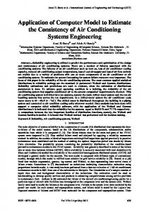
results indicated that the water separator is the component with the most observed failures. This component mostly exhibits a random failure pattern with a high rate, except for a short period in early life, in which increasing failure rate predominates. Salem Bahri [9] presented work extended the classic availability model to a new asymptotic availability model when the failure and repair rates are distributed according to the Weibull model. Nishida [10] described reliability of a Data-center air conditioning system, especially in the viewpoint of the relationship between the reliability and the air conditioning power supply. They examined the system reliability including the air-conditioning power supply in detail, and proposed a new factor for evaluating the reliability of the power configuration of the air conditioning system in this report. The Failure Process Modelling plays a fundamental role in reliability analysis of components and systems. Regattieri [11] determined Complex methodologies using false assumptions such as constant failure rates, statistical independence between components, renewal processes and others, Their misconceptions resulted in poor evaluation of the real reliability performance of components and systems, the study showed that a correct definition of the model describing the failure mode is a very critical issue and requires efforts often not sufficiently focused on by engineers. The two new maintenance concepts have been introduced by Tiedo Tinga [12], that combines the benefits of traditional static concepts and condition based maintenance. The new concepts, usage based maintenance (UBM) and load based maintenance (LBM), apply usage or load parameters that were monitored during service to perform a physical model-based assessment of the system condition [13]. II. MODELS AND METHODS Air conditioning equipment can take many forms. The method used for most single family homes is a split system central air conditioner using a vapour compression cycle. This air conditioning system is composed of both an outdoor and an indoor unit. The outdoor unit is a condensing unit composed mainly of a compressor, condenser coils, and a fan. Homes that have forced air furnaces typically have an indoor evaporator coil that is embedded within or mounted above the furnace. Homes without forced air furnaces use an air handler composed of an evaporator coil and fan. An air handler (AHU), is a device used to condition and circulate air as part of a heating, ventilating, and air-conditioning (HVAC) system. An air handler is usually a large metal box containing a blower, heating or cooling elements filter racks or chambers, sound attenuators, and dampers. Air handlers usually connect to ductwork that distributes the conditioned air through the building and returns it to the AHU. Sometimes AHUs discharge (supply) and admit (return) air directly to and from the space served without ductwork. A set of refrigerant lines allows the refrigerant to circulate between the indoor and outdoor units as shown in Figure 1.

Fig. 1. Indoor and outdoor units in air conditioning system(13)

Cooling is provided when the liquid refrigerant is delivered to the indoor evaporator coil. The refrigerant begins to evaporate, thus cooling the coil and the air that is blown across the coil. This cold air is blown through the home’s ductwork into the living spaces. After passing through the indoor coil, the heat absorbed from the air causes the refrigerant to vaporize. The refrigerant vapour is drawn outside to the compressor in the outdoor unit. The compressor raises the pressure of the refrigerant and discharges it to the condenser coils. The refrigerant in the coils loses heat to the outside air being blown across the coils causing the refrigerant to condense to a liquid. This liquid then enters the refrigerant lines where it travels back into the home and through an expansion device, which reduces the pressure allowing the refrigerant to vaporize in the evaporative coil, and thus repeat the process. The process is summarized in Figure 2.

ISSN : 0975-4024


660


Fig.2. Diagram of the Basic Refrigeration Cycle(13)

In addition to lowering the dry bulb temperature of the air in the home, central air conditioners are effective at lowering the humidity. Moisture in the air condenses forming water droplets when it comes into contact with the cold evaporator coils. These droplets run off the coil and are discharged to the house’s drain system. Removing the humidity is a big component of increasing the comfort of homes in many areas of the country. This process is referred to as latent cooling, where as the process of lowering the dry bulb temperature is referred to a sensible cooling. A building under study ten departments, it is important to classify the air conditioning system into subsystems in order to analyze the failure data accurately. The air conditioning system of this building is divided into two main parts i.e. the chilled water system and the air handling system. Five chilled-water applied systems uses chilled water to transport heat energy between the airside, chillers and the outdoors. These systems are more commonly found in large HVAC installations, given their efficiency advantages. The components of the chiller (evaporator, compressor, an air- or water-cooled condenser, and expansion device) are often manufactured, assembled, and tested as a complete package within the factory. These packaged systems can reduce field labor, speed installation and improve reliability. Alternatively, the components of the refrigeration loop may be selected separately. While water-cooled chillers are rarely installed as separate components, some air cooled chillers offer the flexibility of separating the components for installation in different locations. This allows the system design engineer to position the components where they best serve the space, acoustic, and maintenance requirements of the building owner. Another benefit of a chilled-water applied system is refrigerant containment. Having the refrigeration equipment installed in a central location minimizes the potential for refrigerant leaks, simplifies refrigerant handling practices, and typically makes it easier to contain a leak if one does occur. The first part, the chilled water system is further divided into 5 subsystems containing the cooling tower (CT), the condenser water pump (CWP), the chiller (CH) and the secondary chilled water pump (SCHWP). Each subsystem is then connected in series to the next subsystem. The abbreviation used for the chilled water system and the subsystems is tabulated as in Table 1. The second part of the air conditioning system is the ten dedicated air handling units, AHU1 to AHU10 serving ten departments. The main components that make up the typical AHU system are the primary filter, the secondary filter, the cooling coil and the blowermotor. The study leads parameter that estimates for two commonly reliable methods: the standard (2 parameter) Weibull and Gamma distributions. Considering fitting of the previous models, as listed for a time–to–failure. The commonly used approach in reliability modelling is to model the time between failures as a random variable. The estimation of future performance of the observed system, it assumed that the time between failures can modelled as a Weibull distributed random variable, with and reliability Rt and probability density function f(t), also cumulative density function. Availability A(t) and maintainability were determined to optimize the true maintenance time for the system. The use of the Gamma distribution still has some value to reliability analysis. As more of an exception than the norm, the distributions can be effectively incorporated into reliability analysis if the constant failure rate assumption can be justified. Additionally, prior efforts and standards that extensively utilized the exponential distribution should be commended for introducing and formalizing the reliability methods that formed the basis of more advanced analysis techniques and for applying more rigorous scientific approaches within the field. Comparison between two distributions is performed to optimize proposed method. A.

III. RESULTS AND DISCUSSION Methods of Modelling (Two parameter Weibull model) The reliability of systems and the ways of calculate it, which consist of, Failure Data collection, Failure representation, simulation and drawing graphically the histogram and probability plot in order to calculate Time Between Failure TBF, Calculate the β-value of Weibull distribution for the plant, analysing the charts to

ISSN : 0975-4024


661


determine the age stage from parts and to calculate the optimistic prediction maintenance time and analysing the effect of failure mode in order to calculate the risk. The Weibull is a very flexible life distribution model. It has reliability R(t) and probability density function PDF and other key formulas given by:

R( t ) = e

t −( ) β

α

, α > 0, β > 0, t ≥ 0

(1)

This model is composed of different Weibull distributions for outdoor and an indoor unit at different time periods each case has a different distribution. The formulas is adopted for other subsystems which represented by chilled water system to calculate the reliability for the subsystems and next the AHU’s ten subsystems which are arranged in series as shown in figure (3). A mathematical expression that describes the reliability of the system, expressed in terms of the reliabilities of its components.

Fig 3. Two component system

So far, we have estimated only static system reliability (at a fixed time)., the system's reliability equation was given by: (2) Rs=R1*R2 The values of R1, R2 were given for a common time and the reliability of the system was estimated for that time as follow: (3) Rs(t)=R1(t)*R2(t) The reliability of the system for any mission time can now be estimated. Assuming a Weibull life distribution for each component, Eqn. (1) can now be expressed in terms of each component's reliability function as follow:

R(t) = e

  t β1  t −t β2     0   −   +     α1   α2   

, t0 ≤ t < ∞

(4)

α the scale parameter β the Shape Parameter t the failure time Since a Company is open 14 hours a day everyday of the year, the reliability is expected to be high. Table 1 and Table 2 that show the time failure for chilled water system and AHUs was obtained from data of air conditioning companies. EasyFit automatically computes the parameter α, β. Table I Time Failure for Chilled Water System

Chilled Water System

Time (hrs)

1

3,000

2

5200

3

4400

4

2200

5

4000

The reliability for Chilled Water System at: α1 = 2.6712 β1 = 3.8792 equal R1 (t)= 86.0527%

ISSN : 0975-4024


662


Table II Time Failure for AHU Systems

AHU

Time (hrs)

1

1,000

2

5000

3

1550

4

1500

5

1000

The reliability for AHU System at: α 2 = 1.6465 β 2= 2.9047 R2 (t)= 99.9527% The reliability for the all System: Rs(t)=86.012% The reliability is expected for chilled water system and AHUs to be at 86.012%. Probability distributions are typically defined in terms of the probability density function. However, once the equation for the reliability of the system has been obtained, the system's pdf can be determined. The pdf is the derivative of the reliability function with respect to time or: β

t 

β  t  −  PDF : f (t ) =   e  α  t α 

β

(5)

Time between failures is readily obtained from the data for the Chilled Water System and AHU Systems. It is considered that the failure. Distribution models based on the Weibull family can be fitted to failure data regression or maximum likelihood methods. In addition to selecting a model to be fitted to the data, along with a fitting method, a criterion used to measure the fit of a model and then determine the one of best fit is required. This PDF function in probability theory, a probability density function (PDF), or density of a continuous random variable is a function that describes the relative likelihood for this random variable to occur at a given point. The probability for the random variable to fall within a particular region is given by the integral of this variable’s density over the region. The probability density function is non-negative everywhere, and its integral over the entire space is equal to one as shown in Figures (4),(5) . Probability Density Function 0.28 0.26 0.24 0.22 0.2

f(x)

0.18 0.16 0.14 0.12 0.1 0.08 0.06 0.04 0.02 0 0

2

4

6

8

x Weibull (2.6712; 3.8792)

Fig. 4. Weibull Distribution for Chilled Water System

ISSN : 0975-4024


663


Probability Density Function 0.26 0.24 0.22 0.2 0.18

f(x)

0.16 0.14 0.12 0.1 0.08 0.06 0.04 0.02 0 0

2

4

6

8

x Weibull (1.6465; 2.9047)

Fig. 5. Weibull Distribution for AHUs

The cumulative distribution function may be defined the same way in the multivariate case., if there are two random variables, X and Y, their (bivariate) cumulative distribution function F(x, y) is defined, for any pair of values x0 and y0, as the probability for a realization of the pair {X, Y} to be such that where X represents chilled water system and Y represent AHUs: β

t −  α 

CDF: F(t) = 1− e

(6)

FXY (x, y) = FX (x).FY ( y)

(7)

< X ≤ x0 y2 CDF for Chilled Water System=1-0.860527=0.139473 CDF for AHU System=1-0.999527=4.73x10-4 CDF for all system=6.597x10-5

X= t1

,

-

-

< Y ≤ y0

IV. GAMMA MODEL The distribution is frequently a probability model for waiting times; for instance, in life testing, the waiting time until death is a random variable that is frequently modeled with a gamma distribution [15,16].α and β for this distribution is concluded by easy fit, its equal (10.186,0.36915)for Chilled Water System and (2.2394,1.3236)for AHUs.The Gamma distribution model has probability density function PDF and reliability R(t) formulas given by t

− 1 PDF : f (t , α , β ) = α t α −1e β β Γ(α )

t>0

(8)

t

CDF : F (t ) =  f (t )dt

, t0 ≤ t < ∞

(9)

0

R(t) = 1− F(t)

(10)

The problem of selecting the best fitting distribution can be easily solved by applying the specialized distribution fitting software EasyFit. This software product is designed to automate the whole distribution fitting process. It performs all the calculations, so you just need to interpret the analysis results and actually select the best model. The system's reliability equation bas on Gamma distribution was given by: Rs=R1*R2 (11) The values of R1, R2 were given for a common time and the reliability of the system was estimated for that time as follow: (12) Rs(t)=R1(t)*R2(t) The reliability for Chilled Water System at: α1 = 10.186 β1 = 0.36915

ISSN : 0975-4024


664


equal R1 (t)= 99.6% The reliability for AHU System at: α 2 = 2.2394 β 2= 1.3236 R2 (t)= 77.7% The reliability for the all System: Rs(t)=77.38% Gamma cdf at each of the values in using the corresponding shape parameters and scale parameters in β, α, β can be vectors, matrices, or multidimensional arrays that all have the same size. α scalar input was expanded to a constant array with the same dimensions as the other inputs. The parameters α and β must be positive. The gamma cdf is the probability that a single observation from a gamma distribution with parameters could be computed as follow CDF for Chilled Water System=1-0.996=4x10-3 CDF for AHU System=1-0.7738=4.73x10-4 CDF for all system=6.597x10=0.226 The probability density function of Gamma distribution was also non-negative everywhere, and its integral over the entire space is equal to one as shown in Figures (6),(7) . Probability Density Function 0.36 0.32 0.28

f(x)

0.24 0.2 0.16 0.12 0.08 0.04 0 0

2

4

6

8

x Gamma (10.186; 0.36915)

Figure (6) Gamma Distribution for Chilled Water System

Figure (6) Gamma Distribution for AHUs

It is very important to select the best fitting survival distribution, because the model it represents will be used to make key decisions. For example, you cannot assume the Exponential distribution just because it is the simplest one - in fact, it is inappropriate in many cases. The use of incorrect models can lead to serious problems such as damage of expensive equipment, premature failures of products resulting in unsatisfied customers etc.

ISSN : 0975-4024


665


The best way to prevent possible modelling errors, develop more valid models, and thus make better decisions, is to apply distribution fitting. This technique allows to select the probability distribution which best describes the reliability of a component or system, based on available historical data (observed survival times). However, the use of distribution fitting is connected with complex calculations which require special knowledge in the field of statistics and/or programming skills [18]. The problem of selecting the best fitting distribution can be easily solved by applying the specialized distribution fitting software EasyFit. This software product is designed to automate the whole distribution fitting process. It performs all the calculations for you, so you just need to interpret the analysis results and actually select the best model. EasyFit automatically estimates parameters of the chosen distributions [19]. When comparing distributional models, several distributional fits provide comparable values. For Weibull and Gamma may both fit a given set of reliability data quite well? Typically, that was, Weibull be preferred over a Gamma distribution. It may not need to know if the distributional model is optimal, only that it is adequate for the studied purposes. That was, may be able to use techniques designed for normally distributed data even if other distributions fit the data somewhat better [20]. V. AVAILABILITY A(T) An item or system is specified, procured, and designed to a functional requirement and it is important that it satisfies this requirement. However it is also desirable that the item or system should be predictably available and this depends upon the reliability and availability. For items and systems used in this study, the availability, reliability and maintainability considerations are vital. The economic justification for any project is generally based on the lifetime cost of the air condition system. A major contribution to this cost involves an evaluation of the availability reliability and maintainability of the system. Availability = Uptime / (Downtime + Uptime) The time units are generally hours and the time base is 1 year. There are 8760 hours in one year

A(t ) =

UPTime MTBF (13) = UPTime + DownTime MTBF + MTTR

A(t)=0.5895 Where, up Time MTBF Mean Time between Failures down Time MTTR Mean Time. It is noted that the relationship between the equation and maintenance times by reliability and reflects the probability that the system is available and that is to optimize the availability, it must reduce maintenance time. VI. MAINTAINABILITY One of the chief characteristics of reliability; the suitability of system for the various procedures involved in technical servicing and repair. Maintainability is determined by the equipment’s operating and repair effectiveness. Operating effectiveness is the suitability of the equipment for procedures carried out during technical servicing and when the equipment is being prepared for operation, when the operation is in progress, and after the operation is completed. Repair effectiveness is the suitability of the equipment for rapid and convenient repair. In the narrow sense of the word, maintainability is the suitability of equipment for rapid and convenient performance of specific production operations when the equipment is being serviced and repaired, when its technical condition is being monitored, and when its components are being dismantled, checked, replaced, and reassembled. When equipment is being designed and manufactured, maintainability is ensured by correctly selecting the design and performing all manufacturing operations exactly as specified. When equipment is being operated, maintainability is ensured by an efficient system of technical servicing and repair. Maintainability is characterized by the average time needed to return equipment to operating condition, the probability of returning equipment to working condition within a given period of time, operational readiness, utilization factor, interchangeability, and the degree of standardization. The maintainability is expressed as following exponential distribution as shown in figure (6):

M (t) = 1 − e

  1    −   MTTR

= 1 − e−tt

(14)

Where M(t)= Maintainability MTTR=Repair Time The extended use of the following distribution includes maintenance by reducing the cost to a minimum. To get the best time at which replacement occurs analyzes the adoption of preventive maintenance. Weibull is possibility to know which part of the system needed for such maintenance to prevent maintenance only.

ISSN : 0975-4024


666


Figure (6) Maintainability exponential distribution

The bathtub curve is widely used in reliability engineering as shown in figure (7). It describes a particular form of the hazard function which comprises of three parts: •

The first part is a decreasing failure rate known as early failure.

•

The second part is a constant failure rate, known as random failures.

• The third part is an increasing failure rate, known as wear-out failures. The failure rate is high but rapidly decreasing as defective products are identified and discarded, and early sources of potential failure such as handling and installation error are surmounted [17].

Fig.7. Bathtub curve

VII. CONCLUSION The work illustrates the failure mode of air conditioning system. The Weibull and Gamma distributions were used to define (α) the scale parameter and (β) the shape parameter, mean time to failure MTBF failure rate and reliability R(t). Determine the failure mode that no existing maintenance task. The conclusion of this study is improved by adding the maintenance task to prevent the failure. The reliability of the system is increased. To determine the reliability, the maintenance interval depends on the planned maintenance program of the system. A comparison between Weibull and Gamma was studied, Gamma distribution may offer a good fit to some sets of failure data. It is not, however, given as a good reliability results. The study indicated that was a different between the two distributions. Values of the reliability by Weibull equal 86.012%. Weibull model provided good basis for decision making work illustrates the failure mode of air conditioning system. REFERENCES [1] [2]

[3]

R. Corporation, “System analysis reference: reliability availability and optimization”- Reliasoft Publishing, 2012. K. Ro-Yeul, A. Takakusagib, S. Jang-Yeul, S. Fujiic, P. Byung-Yoon Parkd, “Development of an optimal preventive maintenance model based on the reliability assessment for air-conditioning facilities in o'ce buildings” Building and Environment, vol. 39, pp.1141 – 1156, 2009. S.O.T. Ogaji, R. Singh. Advanced engine diagnostics using artificial neural networks. Applied Soft Computing vol. 3,pp. 259–271, 2003.

ISSN : 0975-4024


667


[4] [5] [6] [7] [8] [9] [10] [11] [12] [13] [14] [15] [16] [17] [18] [19] [20]

F.I. Khan M. Haddara. “Risk-based maintenance (RBM): a quantitative approach for maintenance/inspection scheduling and planning”. Journal of Loss Prevention in the Process, Industries; vol. 16, pp. 561–573, 2011. Y.S. Dai M. Xie K.L. Poh G.Q. Liu. A study of service reliability and availability for distributed systems. Reliab Engng Syst Safety; vol. 79 pp.103–112, 2003. D.L. Burrell, S. Low Choy and K.L. Mengersen(2009) “How Reliable is My Reliability Model?” 18th World IMACS / MODSIM Congress, Cairns, Australia pp. 13-17 July. M. Burhanuddin, A. Rahman M. Ahmad, I. Ataharul, A.S. Prabuwono “Reliability Analysis of Repair Time Data Using SemiParametric Measures” European Journal of Scientific Research ISSN 1450-216X, vol.33 No.4 pp.691-701, 2009. A.Z. Al-Garni, M. Tozan, A.M. Al-Garni, and A. Jamal," Failure Forecasting of Aircraft Air-Conditioning/Cooling Pack with Field Data", AIAA Journal of Aircraft, Vol. 44, No. 3, pp. 996-1002, 2007. S. Bahri, F. Ghribi, H. B. Bacha(2009)” A Study of Asymptotic Availability Modeling Availability Modeling for a Failure and a Repair Rates Following a Weibull Distribution.” R&RATA, vol.2, pp.30-42., 2009. R. Nishida, S. Waragai, K. Sekiguchi, M. Kishita, M. H.Miyake, T. Uekusa, “Relationship between the reliability of a Data-center airconditioning system and the air-conditioning power supply.” Telecommunications Energy Conference, pp.1-15, 2008. A. Regattieri,n, R.Manzini, D.Battini “Estimating reliability characteristics in the presence of censored data: A case study in a light commercial vehicle manufacturing system” Reliability Engineering and System Safety, vol. 95, Issue 10, pp. 1093-1102, 2010. T. Tinga. Application of physical failure models to enable usage and load based maintenance” Reliability Engineering and System Safety vol. 95, Issue 10, pp. 1061-1075, 2010. R. V. Hogg and A. T. Craig. “Introduction to Mathematical Statistics”, 4th edition. New York: Macmillan, 1978. A. Rehman, “Machine Learning based Air Traffic Control Strategy”, International Journal of Machine Learning and Cybernatics, 2012, DOI: 10.1007/s13042-012-0096-6. T. Saba and A. Rehman “Effects of Artificially Intelligent Tools on Pattern Recognition”, International Journal of Machine Learning and Cybernetics, 2012, DOI: 10.1007/s13042-012-0082-z. A. Rehman and T. Saba “Neural Network for Document Image Preprocessing” Artificial Intelligence Review, 2012, DOI: 10.1007/s10462-012-9337-z. T. Saba, A. Rehman and G. Sulong “Cursive Script Segmentation with Neural Confidence” International Journal of Innovative Computing, Information and Control (IJICIC), vol. 7, issue 8, pp. 4955-4964, 2011. T. Saba, A. Rehman and G. Sulong (2011) “Improved Statistical Features for Cursive Character Recognition” International Journal of Innovative Computing, Information and Control (IJICIC) vol. 7, No. 9, pp. 5211-5224. A. Selamat, C. Phetchanchai, A. Rehman and T. Saba. “Index Financial Time Series Based on Zigzag-Perceptually Important Points”. Journal of Computer Science, vol. 6 (12): pp. 1389-1395, 2010. A. Rehman and T. Saba (2011). “Performance Analysis of Segmentation Approach for Cursive Handwritten Word Recognition on Benchmark Database”. Digital Signal Processing (Elsevier) Vol. 21, pp. 486-490.

ISSN : 0975-4024


668