Application of Direct and Large Eddy Simulation to

AGARD-CP-551

in in CL O Q EC <
*,

1.50'

+

I

-t-

+

13

14

1.00' 0.75'

Ü

o

0.50' 0.25 0 -

i

i

■

,

, , ...... . . wavenumber,

i

I

i

,

10

11

12

15

K

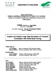
Figure 3. Prediction of Kolmogorov's 5/3 law and Kolmogorov's constant in forced homogeneous isotropic turbulence at steady state : DLM(k) + : DLM(+) : DM.

1-4

source of backscatter. Therefore, it seems reasonable that backscatter should be modeled by a stochastic force. Some subgrid scale models have been proposed that add a stochastic forcing to a purely dissipative viscous term. Chasnov[15] extensively studied the influence of this "eddy forcing" in LES of isotropic turbulence within the framework of the EDQNM approximation. The inclusion of the eddy-forcing term significantly improved the results. The influence of adding such a stochastic term to the Smagorinsky model has also been explored in the context of boundary layers[17] and plane mixing layers[18]. In the model presented here, stochastic backscatter is included in the dynamic model framework which includes local determination of all the coefficients. We model the subgrid scale force as

£

/h

e

"

(8)

where £ is the net energy transfer rate from the resolved to unresolved scales and At is the time-step. This model is very similar to the one used by Leith[18], with the important difference that we determine C\ and Cj dynamically. The simplest choice for e2- is a normalized (dimensionless) white noise in space and time. The net energy transfer rate £ can be determined as follows. The net transfer is the difference between the eddy-dissipation and the backscatter rates. Therefore, £ = C1 £l/3 A4/3 |5|2 - \c\ £

(9)

so that £=

2C\ A4/352

3/2

2+q

(10)

Since /2; enters as a force in the LES equations rather than as a stress tensor, some modification is needed in the usual dynamic procedure. This is implemented by converting Eq. (1) into a vector rather than a tensor relation by taking the divergence of each side. 3.2. Alternative minimization procedures We have mentioned in the previous section that the stochastic backscatter formulation requires the use of the divergence of Eq. (1). Since the sgs stress itself never appears in the LES equations except as a divergence, there is no reason to search for a good model for r,-j. A good description of its divergence is more appropriate. In current formulations one attempts to make an optimal choice for a single parameter C so as to "best satisfy" five scalar equations. In the divergence formulation only three scalar equations need be satisfied. It is therefore reasonable to expect that the C field in the divergence formulation would have less variability in space. One may take the argument one step further and work at a scalar level. Indeed, it is likely that the critical feature in

sgs modeling is to correctly determine the dissipation rate rather than have an accurate model for the sgs stresses. Clark et al. [19] have compared Smagorinsky's model and the "exact" sgs stresses computed by DNS. They found that the correlation coefficient between 2vtSjj and TJJ was as_low as 0.37. However, the correlation between 2diviS[i and djT^j was 0.43 and between 2«,-ö,-^5.tj and liidjTjj was 0.7. Thus, even though the Smagorin sky model is not a good model for the local subgrid scale stresses, its account of the rate of kinetic energy dissipation is reasonably accurate. Inspired by these results, one may base the dynamic procedure for determining the dimensionless coefficients in any subgrid scale model on the scalar equation obtained by multiplying the velocity with the divergence of Eq. (1) In this case, some information on the dynamic evolution of the large scale field will be lost, but it allows the model to be optimized for a good description of the energy transfer rate. The vectorial and scalar versions of Eq. (1) are presently being investigated for the constrained variational formulation. They both lead to integro-differential equations for the coefficient C. Preliminary results in isotropic turbulence show that the probability distribution of C is not strongly altered by using the vectorial or scalar identities, but tests in complex flows are necessary to further discriminate between the various models. 4. APPLICATIONS IN COMPLEX FLOWS The dynamic model has been highly successful in benchmark tests involving homogeneous and channel flows (c.f. Refs. [2, 3, 8, 11]). Having demonstrated the potential of the dynamic model in these simple flows, the overall direction of the LES effort at CTR has shifted toward an evaluation of the model in more complex situations. The general objective of these simulations is to evaluate the effectiveness of the dynamic model as an engineering tool for flows (or flow regions) where Reynolds averaged approaches have faced difficulties. The current test cases do not necessarily take place in complex geometries, but the flow fields contain complex turbulent phenomena that are very difficult to model successfully via Reynolds averaged approaches. Flows currently under investigation include a backward-facing step, wake behind a circular cylinder, airfoil at high angles of attack, separated flow in a diffuser, and boundary layer over a concave surface. Some results from the backward-facing step and concave surface boundary layer are presented below. 4.1. Backward-facing step Large Eddy Simulations have been performed for turbulent flow over a backward facing step at Reynolds number 28000 based on the inlet free-stream velocity and step height. The flow is complex by virtue of the massive separation behind the step, the associated adverse pressure gradient and the recovery downstream of the reattachment region. The LES results are compared with experimental results of Adams et al. [20]. The subgrid scale model used in the calculations is the constrained variational model.

1-5

The experimental facility used by Adams et al. consists of a single sided expansion with a fixed upper wall. The expansion ratio is 1.25 (upstream channel width is 4 step heights). The flow upstream of the step consists of two developing boundary layers, each of thickness roughly 1.2 step-heights. A potential core exists between the boundary layers. An aspect ratio (spanwise extent/step height) of 11.4 was used in order to enhance two-dimensionality of the mean flow in the separated region. The computational domain starts 10 step-heights upstream of the step in order to allow the flow to recover from the inflow boundary condition, and extends 20 step-heights downstream of the step. The spanwise extent of the computational domain is 3 step heights. As in the experiment, a solid wall is used at the top boundary. The inflow boundary condition consists of a mean velocity profile with superimposed random fluctuations [21]. A convective boundary condition is used at the domain exit. In the homogeneous spanwise direction periodic boundary conditions are used and no slip conditions are employed along all solid walls. The computational mesh is uniform in the spanwise direction and stretched in both the streamwise and wall-normal directions. Wall-normal stretching of the mesh is necessary in order to be able to resolve the boundary layers. The mesh in the wall-normal direction is designed to resolve the boundary-layers upstream as well as downstream of the step. The mesh is also stretched in the streamwise direction, increasing the density of grid-points around the corner of the step. This is necessary in order to resolve sharp mean gradients in that region. Earlier simulations clearly demonstrated the need for adequate streamwise resolution at the corner of the step. The computational mesh has 244x96x96 grid points in the streamwise, wallnormal and spanwise direction, respectively. Based on the friction velocity at the inlet of the domain, the resolution (in wall units) in the streamwise direction is : Ax+ ■ = 17 and Ax^ax = 273. The minimum resolution occurs at the corner of the step. For the wall-normal „+nm 1. direction the corresponding numbers are : Ay^ and Ay^iax = 227. The spanwise (uniform) resolution is Az+ = 36. The calculation required about 70 CPU hours on a CRAY-C90. Evaluation of the subgrid scale model increases the CPU time spent per time step in the code by about 30%. An important parameter for comparing the results of the backward facing step flows is the reattachment location. Adams et al. report a reattachment length of 6.7 step heights which is identical to the value calculated in the present simulation. Figure 4 shows the mean streamwise velocity profiles at three locations downstream of the step. x/h = 4.5 is in the recirculation region, x/h = 7.2 is in the reattachment region and x/h = 12.2 is in the recovery region. Overall good agreement between the computation and experiment is observed at all locations. The slight lag of the LES velocity profile compared with the experimental values in the recovery region is believed to be due to the blocking effect of the side-wall boundary layers in the experiment. Figure 5 shows the streamwise turbulent

U/UQ

Figure 4. Mean streamwise velocity profiles downstream of the step. : LES; o : experimental results of Adams et al. [20]

Si

U'/UQ

Figure 5. Streamwise turbulence intensities downstream of the step. : LES; o : experimental results of Adams et al. [20] intensity. As with the mean velocity profiles, the overall agreement between the experiment and computation is excellent. 4.2. Concave surface boundary layer Large eddy simulations of a turbulent boundary layer on a concave surface at momentum thickness Reynolds number of 1300 have been performed. Although the geometry of a concave wall is not very complex, the boundary layer that develops on its surface is difficult to model due to the presence of streamwise Taylor-Görtler vortices. These vortices arise as a result of a centrifugal instability associated with the concave curvature. The vortices are of the same scale as the boundary layer thickness, alternate in sense of rotation, and are strong enough to induce significant changes in the boundary layer statistics. Owing to their streamwise orientation and alternate signs, the Taylor-Görtler vortices induce alternating bands of flow toward and away from the wall. The induced upwash and downwash motions serve as effective agents to transport streamwise momentum normal to the wall, thereby increasing the skin friction. As evidenced by the 1980 AFOSR-Stanford conference on complex turbulent flows, Reynolds averaged models perform poorly for concave curvature since the Taylor-Görtler vortices

1-6

are not resolved in these calculations. Historically the ad hoc corrections for the effects of curvature have been unsatisfactory.

The computational grid contains 178 x 40 x 64 points in the streamwise, wall-normal, and spanwise directions respectively. The mesh is stretched in the wall-normal direction and uniform in the other two.

The flow solver is a variant of the code described by Choi and Moin[22]. The incompressible Navier-Stokes equations are solved in a coordinate space where two directions are curvilinear and the third (spanwise) direction is Cartesian. Spatial derivatives are approximated with second-order finite differences on a staggered mesh. A fully-implicit second-order fractional step algorithm is used for the time advancement.

In order to eliminate starting transients, the simulation is run for an initial period of 60 boundary layer inertial time scale units (1.7 flow-through times). Statistics are then sampled over a period of 300 inertial time scales (8.5 flow-through times). Mean quantities are formed by averaging over both the spanwise direction and time.

The algebraic formulation of the dynamic model is used with test filtering being restricted to the streamwise and spanwise directions. The equations for the Smagorinsky coefficient are averaged over the spanwise direction. In this simulation, the number of grid points in the spanwise direction is not large enough to ensure that the model coefficient is always positive. For this reason, the constraint is imposed that the total viscosity (eddy plus molecular) remain non-negative. In this case, the constraint binds for less than 0.01 % of the points within the domain.

Mean velocity profiles at several streamwise stations are compared with the experimental data in Figure 6. The first station is on the flat inlet section, 8 boundary layer thicknesses ahead of the curved section. The other 4 stations are at 15°, 30°, 45°, and 60° (4.7, 9.5, 14.2, and 18.9 boundary layer thicknesses into the curved section). Overall the agreement between simulation and experiment is good. Near the start of the curve, the simulation produces profiles that are a bit fuller near the wall as compared with the experiment. The fuller profiles also result in higher skin friction as compared with the experiment up to about 30° into the the curve.

The LES corresponds to the water-tunnel experimental configuration of Barlow and Johnston[23] and Johnson and Johnston [24]. In the experiment, the boundary layer develops on a long flat entry section and is then subjected to a 90° constant radius of curvature bend. In the simulation, the calculation begins approximately 10 boundary layer thicknesses upstream of the curved section and ends at the 75° station (the boundary layer thickness measured at the onset of curvature, profile along the lower wall. x proposed model, A shifted model, experimental data in [25], experimental data in [26]

with the value 1.33 reported by Gavrilakis, [21]. For case 2 this ratio was 1.18. Brandrett and Baines [13] reported a value of Uc/Ub = 1.2 for a higher Reynolds number (Reb = 80000). The predicted values are also consistent with the trend given by Demuren and Rodi [24], meaning that the value of UcjUb is decreasing as the Reynolds number increases. In figure 4 the mean secondary flow velocity vectors averaged over the four quadrants, are given for case 1 and case 2. The magnitudes of the maximum secondary velocity were found to be 2.51% and 2.23% of the bulk velocity accordingly. The second one is in good agreement with the value of 2.2% reported in [13]. For the low Reynolds number case Gavrilakis predicted

1

1

(a) 20

A

r

*^~-*-^

1.0 W

Ä—____K

\

■

0.0

0.2

0.4

A

0.5

- /

'

0.6

•

I

i

I

i

s

-

_

t

—«:—*—rf

f /

I:

:

'

/ / ' / / S '

I '/// ' • / / /

Fig. 4:

f

v

^ >

f,

-

A J

8

0.

(c)

—r—r—r—7—7-

0.0 0.0

j ' ~~^ v \f t t 1 f ." ~~ V V I f I ' ' 'Mil//" \ , v V \ f t f ' "

\ , V t f f t '"^

\ '///"'ZZ

Fig. 6: \ I /1

0.2

0.4

0.6

Turbulent intensities along the normal wall bisector at ReT = 150. x case 1, A Smagorinsky model DNS data [21], (a) Urms, (b) (c) Wrr, V„

// I

Mean secondary velocity vectors at a quadrant. Left: case 1, Right: case 2

a relatively lower value of 1.9%. The difference could be due to the limited resolution, since in case 2 the number of points at the cross section is marginal to capture all details of the secondary flow. The distribution of rw/ < rw > along the lower duct wall for case 2 is given in figure 5. The measured values in [25]

2-5 2.50 2.00 1.50 1.00 0.50 0.00

0.2

0.0

1.00 0.75

'

i

0.8

0.6

0.4 '

1

I

(b)

Frr«x 0.C217

*

0.50 0.25

- A

»

~&T

1

~/r

-*

— JC _

a -a-'

1

Fig. 8:

Fig. 7:

Isolines of model coefficient at a quadrant for case 2

Normal Reynolds stresses along the normal wall bisector at ReT = 1125. x case 2, A Smagorinsky model experimental data in [13], experimental data in [22], (a) uu, (b) vv, (c) ww

and [26] at Reb = 50000 and Reb = 34000 respectively, are also included. The prediction given by the new wall model is in good agreement with the experimental data. It follows quite closely the measured values with a midwall value of 1.005 < TW >. For case 1 the mid-wall value was 1.12 < rw >; slightly lower than the one reported in [21], which is 1.18 < rw >. The computation for case 2 was repeated using the shifted model [15] as approximate wall boundary condition. The resulting TW/ < TW > distribution is also given in figure 5. It can be seen that the predicted value close to the corner region is higher than the measured one, probably because in this region the average streamwise velocity is far from satisfying the log-law which is required by the model. In figure 6 and 7 the normal Reynolds stress profiles along the normal wall bisector are given for case 1 and 2 respectively. The choice of the velocity scales is different for each case, in order to be able to have comparisons with the reference data, minimizing the uncertainties introduced by rescaling the data using empirical correlations. The local shear velocity (referred as u*) is chosen for case 1 and the bulk velocity Ub for case 2. In figure 5 the velocity fluctuations obtained with the dynamic model compare well with the DNS data, [21]. An improvement can be observed compared with the Smagorinsky model. A similar behaviour can be seen in fig 7 for case 2, which is more evident probably due to the lower resolution. For both cases the Smagorinsky model is performing purely mainly in the wall region. This can be attributed to the less dissipative character of the dynamic model in this region. In figure 8 isolines of < C > are given at a quadrant. In the centerline region < C > varies between 0.012 - 0.020, corresponding to Cs values of 0.11 - 0.14, which are very close to the value oiCs =0.12 used in the actual Smagorinsky computation. Approaching the solid boundaries, C is reduced rapidly and reaches a value of approximately 0.004, corresponding to Cs = 0.06 which is half of the one used in the simulation.

jg§Brf«MSg|fgSff< ä^tesSiraSSyr^—^^

Fig. 9:

Streamwise two point correlations for case 1. The symbols denote LES data, the lines denote DNS data [21], x Ru, A

A22,D

Ä33

In figure 9 two point streamwise correlations are given for case 1. The agreement with the DNS data is very good despite the mesh coarseness in this direction.

6

CONCLUSIONS

In the present study, the dynamic eddy viscosity model was used in finite difference computations of turbulent flow in a square duct at high Reynolds numbers. The accuracy and suitability of the model for such flow cases was demonstrated. The mean velocity field and low order turbulent statistics compare well with the reference data. A considerable improvement can be observed for most of the statistics in comparison with the Smagorinsky model. The line averaging performed to eliminate ill-conditioning and make the model mathematically self-consistent, was found to be more accurate and robust than a straitforward localization procedure used in a previous study [20]. However, this averaging procedure is limiting the applicability of the model to flows were at least one homogeneous direction exists. For flows in which no homogeneous direction is available, a localized model should be introduced. An other issue addressed in this study is the accuracy and suitability of approximate wall boundary conditions, which could be crucial in extending LES to complex wall bounded flows at high Reynolds numbers. The proposed model was found to be more accurate than existing models in such flow cases. However, a more sophisticated tur-

2-6 bulence model able to account for the complicated flow phenomena present in the wall region is more desirable and could improve the accuracy of the model. Further developments in both fields mentioned above are quite important in extending LES to engineering applications. Considering also the flexibility of finite difference methods in complex geometries and the fact that the cost of the simulations reported in this study is not exiting 15ft on a fast desktop workstation, LES can be considered a promising tool for the prediction of practical flow problems at high Reynolds numbers.

ACKNOWLEDGMENTS This work is supported by E.E.C. under grand No. ERBCHDICT930257. The authors are grateful to Prof. TJ. Piomelli for many useful discussions during the coarse of this work, and to Dr. S. Gavrilakis for kindly providing detailed data from his DNS.

REFERENCES [1] J. W. Deardorff. A numerical study of threedimensional turbulent channel flow at large Reynolds numbers. J. Fluid Mech., 41:453-480, 1969. [2] J. Smagorinsky. General circulation experiments with the primitive equations, i. the basic experiment. Mori. Weather Rev., 91:99, 1963. [3] U. Piomelli, H. Cabot, P. Moin, and S. Lee. Subgridscale backscatter in turbulent and transitional flows. Phys. Fluids A, 3(7):1766-1771, July 1991. [4] M. Germano, U. Piomelli, P. Moin, and W.H. Cabot. A dynamic subgrid-scale eddy viscosity model. Phys. Fluids A, 3(7):1760-1765, July 1991." [5] M. Germano. Turbulence : the filtering approach. J. Fluid Mech., 238:325-336, 1992. [6] K. Akselvoll and P. Moin. Application of the dynamic localization model to large eddy simulation of turbulent flow over a backward facing step. In Engineering applications of large eddy simulations, editor, S. A. Ragab and U. Piomelli. The Amarican Society of Fluids Engineering, New York, 1993. [7] W. H. Cabot and P. Moin. Large eddy simulation of scalar transport with the dynamic subgrid-scale model. In Large eddy simulation of complex engineering and geophysical flows, editors, B. Galperin. and S. Orzag. Cambridge University Press, Cambridge, 1993. [8] Y. Zang, R. L. Street, and J. R. Koseff. A dynamic mixed subgrid-scale model and its application to turbulent recirculating flows. Phys. Fluids A, 12(5):3186-3196, December 1993. [9] P. Moin, K. Squires, W. Cabot, and S. Lee. A dynamic subgrid scale model for compressible turbulence and scalar transport. Phys. Fluids A, ll(3):2746-2757, November 1991. [10] U. Piomelli. High Reynolds number calculations using the dynamic subgrid-scale stress model. Phys. Fluids A, 5(6):1484-1490, June 1993.

[11] E. Balaras, C. Benocci, and U. Piomelli. Finite difference computations of high Reynolds number flows using the dynamic subgrid-scale model. Theoretical and Computational Fluid Dynamics, 1994. submitted for publication. [12] C. G. Speziale. The dissipation rate correlation and turbulent secondary flows in noncircular ducts. J. Fluids Eng., Transactions of ASME, 108:118-120, 1986. [13] E. Brundrett and W. D. Baines. The production and diffusion of vorticity in a duct flow. J. Fluid Mech., 19:375-394, 1964. [14] F. B. Gessner. The origin of secondary flow in turbulent flow along a corner. J. Fluid Mech., 58:1-25, 1973. [15] U. Piomelli, J. Ferziger, P. Moin, and J. Kim. New approximate boundary conditions for large eddy simulations of wall-bounded flows. Phys. Fluids A, 1(6):1061-1068, June 1989. [16] G. Bagwell, R. J. Andrian, R. D. Moser, and J. Kim. Improved approximation of wall shear stress boundary conditions for large eddy simulation. In Near wall turbulent flows, editor, C. G. Speziale and B. P. Launder, pages 265-275. Elsevier Science Publishers, 1993. [17] J. Kim, P. Moin, and R. Moser. Turbulent statistics in fully developed channel flow at low Reynolds number. J. Fluid Mech., 177:133-166, 1987. [18] E. Balaras, C. Benocci, and P. F. Trecate. A new model for estimating the wall shear stress in large eddy simulations. In Proceedings of international workshop on large eddy simulations of turbulent flows in engineering and the environment, Montreal, Quebec. Canada, September 27-28 1993. CERCA. [19] D. K. Lilly. A proposed modification of the germano subgrid-scale closure method. Phys. Fluids A, 4(3):633-635, March 1992. [20] E. Balaras and C. Benocci. Large eddy simulation of flow in a square duct. In Proceedings of the thirteenth symposium on turbulence. University of Missuri Rolla, September 21-23 1992. [21] S. Gavrilakis. Numerical simulation of low Reynolds number tutbulent in a straight duct. J. Fluid Mech., 244:101-129, 1993. [22] F. B. Gessner. PhD thesis, Purdue University, 1964. [23] A. Melling and J. H. Whitelaw. Turbulent flow in a rectangular duct. J. Fluid Mech., 78:289-314, 1976. [24] A. O. Demuren and W. Rodi. Calculation of turbulence-driven secondary motion in non-circular ducts. J. Fluid Mech., 140:189-222, 1984. [25] E. G. Lund. Mean flow and turbulence characteristics in the near corner region of a square duct. Master's thesis, University of Washington, 1977. [26] H. J. Leutheusser. Turbulent flow in rectungular ducts. J. Hydraulics Division, 89(HY3):1-19, 1963.

3-1

LARGE-EDDY SIMULATION OF ROTATING CHANNEL FLOWS USING A LOCALIZED DYNAMIC MODEL Ugo Piomelli and Junhui Liu Department of Mechanical Engineering University of Maryland College Park, MD 20742, USA

ABSTRACT Most applications of the dynamic subgrid-scale stress model use volume- or planar-averaging to avoid illconditioning of the model coefficient, which may result in numerical instabilities. A spatially-varying coefficient is also mathematically inconsistent with the model derivation. A localization procedure is proposed here that removes the mathematical inconsistency to any desired order of accuracy in time. This model is applied to the simulation of rotating channel flow, and results in improved prediction of the turbulence statistics.

INTRODUCTION The dynamic subgrid-scale stress model, introduced by Germano et al. [1], has been widely used for the large-eddy simulation (LES) of incompressible and compressible flows. The model is based on the introduction of two filters; in addition to the grid filter (denoted by an overbar), which defines the resolved and subgrid scales, a test filter (denoted by a circumflex) is used, whose width is larger than the grid filter width. The stress terms that appear when the grid filter is applied to the Navier-Stokes equations are the subgrid-scale (SGS) stresses r,j; in an analogous manner, the test filter defines a new set of stresses, the subtest-scale stresses Tij. An identity [2] relates Tij and TJJ to the resolved turbulent stresses, £,;-. If an eddy-viscosity model is used to parametrize r,j and T^, this identity can be exploited to determine the model coefficient. This yields a coefficient that is function of space and time, and whose value is determined by the energy content of the smallest resolved scales, rather than input a priori as in the standard Smagorinsky model [3]. Two difficulties, however, arise in the determination of C: the first is that the model is ill-conditioned because the denominator of the expression for C becomes very small at a few points in the flow. Furthermore, the procedure described above is not mathematically self-consistent since it requires that a spatially-dependent coefficient be extracted from a filtering operation [4]. To overcome

this problem, C is usually assumed to be only a function of time and of the spatial coordinates in inhomogeneous directions. The mathematical inconsistency is thus eliminated, and the ill-conditioning problem is alleviated. The resulting eddy viscosity has several desirable features: it vanishes in laminar flow, it can be negative (indicating that the model is capable of predicting backscatter, i.e., energy transfer from the small to the large scales) and it has the correct asymptotic behavior near a solid boundary. The dynamic eddy viscosity model has been used successfully to solve a variety of flows such as transitional and turbulent channel flows [1, 5], and compressible isotropic turbulence [6]. Since the model coefficient adjusts itself to the energy content of the smallest resolved scales, it can also be applied to relaminarizing or intermittent flows, and has given accurate prediction of problems in which the Smagorinsky model did not work well. Esmaili and Piomelli [7], who used it in the LES of sink flows, observed that C vanishes when the boundary layer relaminarizes even if inactive fluctuations are still present. Squires and Piomelli [8] applied it to rotating flows, and found that C decreases as a result of the stabilizing effect of rotation. Orszag et al. [9] moved a number of criticisms to the dynamic model; in the first place, they attributed its success in the prediction of low Reynolds number flows to the fact that it acts as a damping function for the eddy viscosity in the wall region, where, they state, the test filter width A is in the inertial range and the grid filter width A is in the dissipation range; this results in Tij « Tij and < C,j >~ < r,j >~ y (< • > denotes plane-averaging). It is easy to show analytically that this statement is incorrect since, for most filters of interest, < Tij >>< Tij > independent of the shape of the spectrum. Furthermore, in the wall region, both A and A are in flat regions of the spectrum, and the ratios of dj, Tij and Tij to the resolved energy and stresses become constant [5]. Orszag and coworkers [9] also hypothesized that the model will depend very strongly on the ratio of test to grid filter width, a point that had already been addressed by Germano et al. [1], who showed that the model is rather insensitive to this ratio. Fi-

Paper presented at the 74th Fluid Dynamics Symposium on "Application of Direct and Large Eddy Simulation to Transition and Turbulence" held at Chania, Crete, Greece, in April 1994.

3-2

nally, they conjecture that application of the model may become problematic at high Reynolds numbers; however, Piomelli [5] and Balaras et al. [10] have computed channel flow at Reynolds numbers (based on channel width and bulk velocity) ranging between 5,000 and 250,000 (200 < Re < 5, 000 based on channel halfwidth and friction velocity), obtaining results in good agreement with the data. A limitation of the dynamic model is, however, the plane averaging mentioned above. For flows in which no homogeneous directions exist, the model coefficient should be a function of all spatial coordinates. Even flows that are homogeneous in planes parallel to the wall may be intermittent, in which case the eddy viscosity should be non-zero only in regions of significant turbulent activity, and zero elsewhere, a behavior that is not always possible if plane averaging is performed. Although straightforward localization of the dynamic model gives rise to the problems mentioned above, it has nonetheless been used by Zang and «workers in simulations of the turbulent flow in a driven cavity [11]. They performed some local averaging (over the test filter cell) and also constrained the total viscosity (sum of molecular and eddy viscosity) to be non-negative, thus allowing a small amount of backscatter. Since large (positive and negative) values of the eddy viscosity were observed only in the corner of the cavity, probably due to the low Reynolds number of the flow they studied, neither the local averaging nor the cutoff applied to avoid backscatter affected the results very much. In later work [12] the same authors adopted a mixed model that was also localized in a similar manner. Ghosal and coworkers [13] recast the problem in variational form, obtaining an integral equation for C that they solved iteratively. This removed the mathematical inconsistency, but the overhead associated with the iterative solution of the integral equation could be significant. The ill-conditioning that led to locally large values of C was removed by the integral formulation, and negative values of the model coefficient were avoided by the additional constraint that C > 0. This model was used for the LES of isotropic decay [13] and to study the flow over a backwardfacing step [14], with results in good agreement with

DNS data. In this paper a localized version of the dynamic model will be proposed and implemented in which the mathematical inconsistency is removed only approximately (i.e., to some order of accuracy in time). The present formulation, however, does not require any iteration; thus, its cost, in terms of CPU and memory, is essentially the same as the plane-averaged model. A small amount of backscatter will be allowed, but negative total viscosities will be avoided for numerical stability. The new localized model will be used for the computation of rotating channel flow. System rotation has some important effects on turbulence: for instance, it inhibits energy transfer from large to small

scales; this leads to a reduction in turbulence dissipation and a decrease in the decay rate of turbulence energy. Furthermore, the turbulence length scales along the rotation axis increase relative to those in non-rotating turbulence. The presence of mean shear normal to the axis of rotation may have either a stabilizing or a destabilizing effect, depending on whether the angular velocity and mean shear have the same or opposite signs. In turbulent channel flow, for example, system rotation acts to both stabilize and destabilize the flow. On the unstable side Coriolis forces resulting from system rotation enhance turbulence-producing events, leading to an increase in turbulence levels, while on the stable side Coriolis forces inhibit turbulence production and decrease turbulence levels. The increase in the component energies, however, is dependent on the rotation rate: at sufficiently high rotation rates streamwise fluctuations on the unstable channel wall are suppressed relative to the non-rotating case. The stabilizing/destabilizing effects of rotation on turbulence in channel flow make this problem an attractive test for subgrid-scale models, which are required to capture relaminarization with inactive turbulent motions as well as fully-developed turbulence. In the next Section, the numerical method will be discussed; then the model will be presented and applied to the simulation of rotating channel flow. The results will then be discussed, and conclusions and recommendations for future work will be drawn.

NUMERICAL METHOD In large-eddy simulations the flow variables are decomposed into a large scale (or resolved) component, denoted by an overbar, and a subgrid scale component. The large scale component is defined by the filtering operation: 7(x)= / /(x')G(x,x')rfx',

(l)

JD

where D is the computational domain, and G is the filter function. Appling the filtering operation to the incompressible Navier-Stokes and continuity equations yields the filtered equations of motion, duj ~dt

d

(Uillj) =

1 dp pdxi

+ v dxi

dxj dxj

dxj

+ 2eij3nuj (2) (3)

where e,-^. is Levi-Civita's alternating tensor and ft the angular velocity of the system. The axis of rotation is in the positive z, or £3 direction. The subgridscale stresses, r;;- = U{Uj —Uiüj, need to be modeled to represent the effect of the subgrid scales on the resolved field. Since the small scales tend to be more isotropic than the large scales, their effects can be

3-3

modeled by fairly simple eddy viscosity models of the form [3] -Tkk

2

-2pTSij =-2CA |S|%,

(4)

in which

where < • > denotes plane-averaging. This form of the coefficient has been widely used in LES calculations. In studies of homogeneous isotropic turbulence, averaging is performed over the entire computational domain, and C = C(t) only, whereas averaging over the spanwise direction is used for spatiallydeveloping flows. As mentioned above, a straightforward localization of the model was used in references [11] and [12], in which C was given by (14) with the plane-averaging replaced by a local average over the test filter cell. The problem of the mathematical inconsistency of the localized application of (14) is not addressed in that work, but the results are in good agreement with experimental data; however, the Reynolds number of those calculations is quite low, and the SGS contribution to the stresses is rather small, which makes it difficult to draw definite conclusions from those simulations. Ghosal and coworkers [13] noted that, if C is assumed to be fully dependent on space, the residual cannot be minimized in the least-squares sense locally; therefore, they introduced a constrained variational problem consisting of the minization of the integral of the square of the sum of the residuals over the entire domain, with the additional constraint that C be non-negative. The result was of the form of Fredholm's integral equation of the second kind, that they

3-4

solved iteratively using under-relaxation to improve convergence. In the present work a simpler approach is taken: the expression (12) is recast in the form

c*ßa

2Ca{j = £?■

! (£?■ - C'ßij) atj =-2

(16)

^rnn^mn

The denominator of (16) is positive definite, like that of (14), but has the advantage that it does not involve a difference between two terms of the same order of magnitude. In wall-bounded flows, amnamn becomes small only where the mean shear vanishes (in the freestream of a boundary layer, for example); the numerator is also expected to vanish there. In these regions, moreover, the flow is essentially uniform, so that spurious high values of C obtained from the ratio of very small numbers do not result in large values of the eddy viscosity or of the SGS stresses. There are various ways to obtain C* at timestep n: 1. Use the value at the previous timestep: C* = Cn_1.

(17)

2. Estimate the value at the present timestep by some backward extrapolation scheme: C* = Cn~1 + At

8C 8t

+

(18)

3. Use an iterative scheme: set C* = Cn~l and calculate the left-hand-side of (16); then replace C* with the newly obtained value and repeat the procedure until convergence to the desired order of accuracy is reached.

Cn

dC dt

(15)

where on the right-hand-side an estimate of the coefficient, denoted by C* and assumed to be known, is used. Since C* is known, the sum of the squares of the residual can now be minimized locally; the contraction that minimizes it, in this case, is:

C

In this work, the second approach will be taken; a first-order extrapolation schemes will be used in which dC/dt\n^i is evaluated using an explicit Euler scheme:

t„-

ReT

0 1 2 3 4 5 6 7

177 192 185 176 185 181 175 177

RoT 1.14 0.00 0.54 1.17 1.63 1.14 1.18 1.17

Rob 0.144 0.000 0.069 0.144 0.210 0.144 0.144 0.144

tn-2

(19)

which gives C* = C n-l

+

tn *n— (C"-1 - Cn-2) . tn-l —tn-2

(20)

Equation (17) will be referred to as the "zeroth-order approximation", equation (20) as the "first-order approximation". No attempt was made to use higherorder schemes, since little difference was observed between the results obtained with the first- and zerothorder approximations. Use of an extrapolation scheme such as the one proposed here contains some inherent dangers: numerical instabilities are possible, and the difference between C* and the actual value Cn could be quite large if C varied on a short time-scale. In practice, however, C is a fairly slowly-varying function of time because of the temporal filtering introduced implicitly by the spatial filtering. By eliminating the smallest scales of motion, the highest frequencies are also filtered out. Typically, the time-scale of the structures whose length scale is the filter width is 5 to 10 times larger than the timestep, and this results in long correlation times for C [20]. The coefficient C obtained from (17) or (20) can be either positive or negative. Since negative total viscosities that are correlated over long times can lead to numerical instabilities, the total viscosity was constrained to be non-negative.

RESULTS AND DISCUSSION Calculations were performed for a Reynolds numbers Ret, = Ub{25)/v = 5700 (based on the channel width, 25, and bulk velocity, C/j), and for a range of

Table 1: Summary of the numerical calculations. Case

Cn-

Model

| Length scale

DNS Eqn. (16), (18) Eqn. (16), (18) Eqn. (16), (18) Eqn. (16), (18) Eqn. (14) Eqn. (16), (17) Eqn. (16), (18)

Eqn. Eqn. Eqn. Eqn. Eqn. Eqn. Eqn.

(6) (6) (6) (6) (6) (6) (7)

3-5

1000 Figure 1: Mean velocity in the rotating channel. Reb = 5,700, Rob = 0.144. Firstorder; zeroth order; SML length scale; plane-averaged; x DNS. (a) global coordinates; (b) wall coordinates.

rotation numbers Rot = £1(26)/Ub- A summary of the calculations is shown in Table 1. The initial conditions for the cases with non-zero rotation rates were obtained from equilibrium cases at Q — 0, and were in very good agreement with experimental and DNS data [5]. After rotation was applied the simulations were integrated forward in time to a new steady state, statistics being obtained by averaging over at least 4 dimensionless time units tuT/S. Experimental measurements in this flow exist [15] but at higher Reynolds numbers, whereas a series of DNS calculations was performed by Kristoffersen and Andersson [16] that span the range of fiej and Rob examined in this work. A direct simulation of the intermediate (Rob — 0.144) case was also performed to compare with the LES results. The DNS used 128x129x128 grid points, and was in very good agreement with the DNS results of Ref. [16]. The mean velocity profiles for cases 3 through 6 (i.e., the calculations for Reb = 5,700 and Rob = 0.144) are compared with DNS data in Figure 1. Very little difference can be observed between the various results. The localized models, however, give better prediction of the turbulent fluctuations u" = ui — < Hi > (where < • > from here on denotes averaging over planes parallel to the wall and time), than the plane-averaged model, especially on the stable side of the channel (Figure 2). The localized models are slightly more dissipative than the plane-averaged one (in which backscatter acts to lower the planeaveraged C). This results in better prediction of the quasi-laminar flow on the stable side. The average values of C are shown in Figure 3. There is very little difference between the zeroth- and firstorder approximations. The length scale proposed in Ref. [17] results in smaller values of C, only partially offset by the larger length scale /A; the model is less dissipative than the ones with the standard length scale, as evidenced by the higher levels of u" turbulent fluctuations near the stable wall and of w" in the

Figure 2: Turbulence intensities in the rotating channel. Reb = 5,700, Rob = 0.144. Firstorder; zeroth order; SML length scale; plane-averaged; x DNS. (a) w; (b) v; (c) w.

Figure 3: Average model coefficient. Reb = 5,700, Rob = 0.144. Case 3; case 5; case 6. -7-2 (a) < C >; (b) < C > A ; (c) rms difference

3-6

1.2

i i-o :&2L

■*t^#t

A

.

> 0.8 t

0.0

-*&--•■**+- - -

0.6

V

0.00

0.05

0.10

0.15

0.20

0.25

Ro„

Figure 4: Subgrid-scale stresses Tu- Reb = 5,700. Rob = 0; — Rob = 0.069; Rob = 0.144; Rob = 0.21.

Figure 5: Friction velocity on the two sides of the channel. -f- Experiments; • DNS; a LES, Ref. [21]; A LES, present calculation.

channel center that can be observed in Figure 2. The rms difference between the predicted coefficient C* and the actual value Cn is also shown in Figure 3c (normalized by the average C). The difference is fairly small (less than 5%) throughout the channel, except on the stable side, where it increases because of the low value of < C >; almost no difference can be observed between the zeroth-and first-order approximations.

normalized by the friction velocity in the absence of rotation uTO, is plotted in Figure 5 (the results of the numerical calculations are also tabulated in Table 2).

The average value of C is lower on the unstable than on the stable side, as expected. The maximum value of C corresponds to a Smagorinsky constant Cs ~ 0.1; the SGS stresses on the unstable side (Figure 4) are slightly larger than in the zero rotation rate (about 10% of the resolved ones, vs. 8% in the norotation case) while on the stable side they are about half the value they have when no rotation is applied. As the rotation number is increased, the SGS stress decreases on the unstable side and increases on the stable side, but it never vanishes entirely as it would if the flow relaminarized completely. Full relaminarization on the stable side was observed in experiments [15] and in the LES calculations of Tafti and Vanka [21]; in the DNS calculations of Kristoffersen and Andersen [16] and in the present ones, however, the fluctuations on the stable side remained significant, and the mean velocity never reached the laminar profile, even at large rotation rates and at a Reynolds number at which relaminarization is expected to occur. The friction velocity uT

The LES, DNS and experimental data are in good agreement on the unstable side; in the experiment the bulk velocity was obtained from the volume flow rate, which led to underestimation of the bulk velocity (and an overestimation of Rob) because of the presence of boundary layers on the sides of the channel (see also [16]). A more significant difference can be observed on the stable side, where the numerical results tend to lie close to the extrapolation of the results of experiments in which the flow remained turbulent on the stable side (the dashed line), and are significantly higher than those for fully relaminarized flow (the chain-dot line). Possible reasons for the difference between the experimental and DNS results on the stable side are the relatively small aspect ratio of the experimental apparatus and the fact that the flow was not fully developed, which may have added a streamwise pressure gradient that could have increased the tendency of the flow towards relaminarization. The results obtained with the dynamic model are in much better agreement with the DNS results than those obtained by Tafti and Vanka [21] with the Smagorinsky model, which tended to overdamp the fluctuations on the stable side, leading to excessively low wall stress even at the lower rotation rate they examined.

Table 2: Normalized friction velocity uT/uT>0 on the unstable and stable side. Case

Rob

Unstable

Stable

0 1 2 3 4 5 6 7

0.144 0.000 0.069 0.144 0.210 0.144 0.144 0.144

1.17 1.00 1.13 1.17 1.20 1.15 1.18 1.17

0.80 1.00 0.85 0.79 0.75 0.82 0.77 0.80

Model DNS Eqn. (16), (18) Eqn. (16), (18) Eqn. (16), (18) Eqn. (16), (18) Eqn. (14) Eqn. (16), (17) Eqn. (16), (18)

Length scale Eqn. Eqn. Eqn. Eqn. Eqn. Eqn. Eqn.

(6) (6) (6) (6) (6) (6) (7)

3-7

Figure 8: History of the friction velocity on the upper and lower walls. Rob — 0.210. Stable wall, unstable wall.

Figure 6: Turbulence intensities in the rotating channel. Rob = 0.0, — Rob = 0.069, Rob = 0.144, Rob = 0.210. (a) w; (b) v; (c) w.

llii'iu

I^Hflllii

TTTHTflflfl

*N

370 &^*Z£Sgg&^

Tl N

370 ~z-i

740

yOO

200

J00

•»00

500

I i 11 IXW

*N

700

v?*;

(c)

370

z*

Figure 7: Averaged velocity vectors in the yz-plane at tuT/6 ~ 6, Rob — 0.210. Streamlines are used to visualize the roll cells. The turbulence intensities normalized by the average shear velocity for various rotation rates are shown in Figure 6. The DNS results of [16] show that, on the unstable side, the peak rms streamwise fluctuation is maximum for Rob ~ 0.1 and then decreases; the present calculations show the same trend. At the high rotation rates the formation of roll cells, which has been observed in experiments and numerical simulations, is quite evident. Usually, two strong cells could be observed accompanied, sometimes, by two weaker ones. In Figure 8 the average velocity vectors in the xy planes are shown, averaged over the streamwise directions and 2 realizations. The vortical structures tend to drift both in the y and z directions. The vortices convect high momentum fluid in the downwash region between them, and, as they drift towards the stable wall, the wall stress there can fluctuate significantly. While on the unstable wall the friction velocity (Figure 8) is nearly constant in time, on the stable wall it exhibits an oscillations with a period of about 4 tuT/S time units, and with significant amplitude. Figure 9 shows contours of the u" and v" velocity fluctuations in two xz-planes near the unstable and stable walls. The downwash of the roll cells appears as an elongated region of increased u" and v" velocity

500

1000

1500

2000

Figure 9: Velocity fluctuation contours in the xzplane. Rob = 0.210, tuT/6 ~ 5. (a) u" at y+ = 3.5, unstable wall; (b) u" at y+ — 3.5, stable wall; (c) v" at y+ = 3.5, stable wall. Contour lines are at intervals of ±1 in parts (a) and (b), ±0.07 in part (c). Dashed lines indicate negative contours. fluctuations at z+ ~ 400. On the unstable side the elongated streaky structure typical of wall bounded flows is present, and little effect of the vortices can be observed. When the roll cells move away from the stable wall, the fluctuations in the near-wall layer become extremely small (Figure 10). The flow on the unstable side, however, is not affected much by the roll cell motions.

CONCLUDING REMARKS A new localization procedure for the dynamic eddyviscosity model has been proposed. The localization is only approximate, in the sense that it is based on a Taylor series expansion of the model coefficient in time, in which the time derivatives are evaluated numerically. Nonetheless, it results in more accurate results compared with the plane-averaged formulation of the model. The localization proposed here, moreover, is better conditioned than the original for-

3-8

[2] Germano, M. "Turbulence: the filtering approach." /. Fluid Mech. 238 325, 1992. N 370 ?

[3] Smagorinsky, J. "General circulation experiments with the primitive equations. I. The basic experiment." Monthly Weather Review 91 99, 1963.

740 (b) -sffiEs +

N

370

740

[4] Cabot, W.H. and Moin, P. "Large eddy simulation of scalar transport with the dynamic subgrid-scale model." In Large Eddy Simulation of Complex Engineering and Geophysical Flows, ed. by B. Galperin and S.A. Orszag, (Cambridge University Press, Cambridge) 141, 1993.

(o) N

[5] Piomelli, U. "High Reynolds number calculations using the dynamic subgrid-scale stress model. " Phys. Fluids A 5 1484, 1993.

370

500

1000

1500

2000

Figure 10: Velocity fluctuation contours in the xzplane. Rot — 0.210, case 4, tuT/6 ~ 8. (a) u" at y+ = 3.5, unstable wall; (b) u" at y+ = 3.5, stable wall; (c) v" at y+ = 3.5, stable wall. Contour lines are at intervals of ±1 in parts (a) and (b), ±0.07 in part (c). Dashed lines indicate negative contours. mulation, and does not result in numerical instabilities. The proposed localization has been tested by computing the flow in a rotating channel. Although the grids used are very coarse, the localized model predicts statistics in good agreement with DNS data; some discrepancy between all the numerical results (both DNS and LES) and the experiments can be explained based on the different boundary conditions. First-order accurate localization, which can be performed without any increase in cost or memory, appears to be sufficient to reduce the mathematical inconsistency to acceptable levels. The vortical structures characteristic of rotating flows of this type were captured. Their time evolution has significant effects on the flow field, especially on the stable side of the channel.

ACKNOWLEDGMENTS Research supported by the Office of Naval Research under Grant N00014-89-J-1638. The computer time was supplied by the Pittsburgh SuperComputing Center.

REFERENCES [1] Germano, M., Piomelli, U., Moin, P., and Cabot, W.H. ' A dynamic subgrid-scale eddy viscosity model " Phys. Fluids A 3 1760, 1991.

[6] Moin, P., Squires, K.D., Cabot, W.H. and Lee, S. "A dynamic subgrid-scale model for compressible turbulence and scalar transport." Phys. Fluids A 3 2746, 1991. [7] Esmaili, H. and Piomelli, U. "Large-eddy simulation of relaminarizing sink flow boundary layers." In Near-Wall Turbulent Flows, ed. by R.M.C. So, CG. Speziale and B.E. Launder, (Elsevier, Amsterdam) 287, 1993. [8] Squires, K.D. and Piomelli, U. "Dynamic modeling of rotating turbulence." In press, Turbulent Shear Flows 9, edited by F. Durst, N. Kasagi, B.E. Launder, F.W. Schmidt and J.H. Whitelaw, (Springer Verlag, Heidelberg), 1994. [9] Orszag, S.A., Staroselsky, I., and Yakhot, V.Y. "Some basic challenges for large eddy simulation research." In Large Eddy Simulation of Complex Engineering and Geophysical Flows, ed. by B. Galperin and S.A. Orszag, (Cambridge University Press, Cambridge) 55, 1993. [10] Balaras, E., Benocci, O, and Piomelli, U. "Finite difference computations of high Reynolds number flows using the dynamic subgrid-scale model." Submitted to Theoret. Comput. Fluid Dyn., 1994. [11] Zang, Y., Street, R.L., and Koseff, J. "Application of a dynamic subgrid-scale model to turbulent recirculating flows." CTR Annual Research Briefs, Center for Turbulence Research, Stanford University 85, 1993. [12] Zang, Y., Street, R.L., and Koseff, J. "A dynamic mised subgrid-scale model and its application to turbulent recirculating flows." Phys. Fluids A 5 3186, 1993. [13] Ghosal, S., Lund, T.S., and Moin, P. "A local dynamic model for LES." CTR Annual Research Briefs, Center for Turbulence Research, Stanford University 3, 1993. [14] Akselvoll, K. and Moin, P. "Application of the dynamic localization model to large-eddy simulation of turbulent flow over a backward facing step." In Engineering Applications of Large

3-9

Eddy Simuhtions-1993, ed. by S.A. Ragab and U. Piomelli, (The American Society of Fluids Engineering, New York) 1, 1993. [15] Johnston, J.P., Halleen, R.M., and Lezius, D.K. "Effects of spanwise rotation on the structure of two-dimensional fully developed turbulent channel flow." J. Fluid Mech. 56 533, 1972. [16] Kristoffersen, R. and Andersson, H.I. "Direct simulation of low Reynolds number turbulent flow in a rotating channel." Submitted to J. Fluid Mech., 1993. [17] Scotti, A., Meneveau, C, and Lilly, D.K. "Generalized Smagorinsky model for anisotropic grids." Phys. Fluids A 5 2306, 1993. [18] Zang, T.A. and Hussaini, M.Y. "On spectral multigrid methods for the time-dependent Navier-Stokes equations." Appl. Math. Comp. 19 359, 1986. [19] Lilly, D.K, "A proposed modification of the Germano subgrid-scale closure method." Phys. Fluids A 4, 633, 1992. [20] Lund, T., Ghosal, S., and Moin, P. "Numerical experiments with highly-variable eddy viscosity models." In Engineering Applications of Large Eddy Simulations-1993, ed. by S.A. Ragab and U. Piomelli, (The American Society of Fluids Engineering, New York) 7, 1993. [21] Tafti, D.K. and Vanka, S.P. " A numerical study of the effects of spanwise rotation on turbulent channel flow." Phys. Fluids A 3 642, 1991.

4-1

THE ASYMPTOTIC STATE OF ROTATING HOMOGENEOUS TURBULENCE AT HIGH REYNOLDS NUMBERS Kyle D. Squires* Jeffrey R. ChasnovJ Nagi N. Mansour*&: Claude Cambon§ Center for Turbulence Research Stanford University Stanford, CA 94305, USA

ABSTRACT

aerodynamics.

The long-time, asymptotic state of rotating homogeneous turbulence at high Reynolds numbers has been examined using large-eddy simulation of the incompressible Navier-Stokes equations. The simulations were carried out using 128 x 128 x 512 collocation points in a computational domain that is four times longer along the rotation axis than in the other directions. Subgrid-scale motions in the simulations were parameterized using a spectral eddy viscosity modified for system rotation. Simulation results show that in the asymptotic state the turbulence kinetic energy undergoes a power-law decay with an exponent which is independent of rotation rate, depending only on the low-wavenumber form of the initial energy spectrum. Integral lengthscale growth in the simulations is also characterized by power-law growth; the correlation length of transverse velocities exhibiting much more rapid growth than observed in non-rotating turbulence.

A rotating flow of particular interest in many studies, including the present work, is examination of the effect of steady system rotation on the evolution of an initially isotropic turbulent flow. Aside from the simplifications associated with analysis and computation of homogeneous flows, one of the principal reasons for the interest in this problem is that solidbody rotation of initially isotropic turbulence represents the most basic turbulent flow whose structure is altered by system rotation but without the complicating effects introduced by mean strains or flow inhomogeneities.

INTRODUCTION AND BACKGROUND Study of turbulent flows in rotating reference frames has long been an area of considerable scientific and engineering interest. Because of its importance, the subject of turbulence in rotating reference frames has motivated over the years a large number of theoretical, experimental, and computational studies. The bulk of these studies have served to demonstrate that the effect of system rotation on turbulence is subtle and remains exceedingly difficult to predict. For example, it is well recognized that the standard models for the dissipation rate of the turbulent kinetic energy do not accurately predict the effects of system rotation. Yet, these models are widely used in engineering predictive schemes for technologically important areas such as turbomachinery and rotorcraft 'University of Vermont, Burlington, VT, USA 'The Hong Kong University of Science and Technology, Clear Water Bay, Hong Kong tNASA Ames Research Center, Moffett Field, CA, USA §Ecole Centrale de Lyon, Ecully Cedex, France

For initially isotropic turbulence it is well known that solid-body rotation inhibits the non-linear cascade of energy from large to small scales. Consequently, the turbulence dissipation rate is reduced relative to non-rotating flows and there is an associated decrease in the decay rate of turbulence kinetic energy [1], [2], [3], [4]. Some computations and experiments have also noted an increase in the integral lengthscales along the rotation axis relative to non-rotating turbulence [5], [6], [7], [8]. Increase in the integral lengthscales has been thought by some to be a prelude to a Taylor-Proudman reorganization to two-dimensional turbulence. However, direct numerical simulation (DNS) has demonstrated that, for very rapid rates of rotation, initially isotropic turbulence remains isotropic and three dimensional [3]. The results in Ref. [3] confirm the essential role of nonlinear interactions for the transition towards twodimensional turbulence to occur; such a transition, first studied using a spectral approach, can be started only for intermediate Rossby numbers at sufficiently large Reynolds numbers [6], [9]. While some of the effects summarized above are reasonably well documented, e.g., reduction in the decay rate of turbulence kinetic energy, other features of rotating flows are less well resolved, e.g., the behavior of the integral scales. There are also other fundamentally important questions associated with rotating turbulence which cannot be resolved from previous investigations. For example, while the decrease

Paper presented at the 74th Fluid Dynamics Symposium on "Application of Direct and Large Eddy Simulation to Transition and Turbulence" held at Cltania, Crete, Greece, in April 1994.

4-2

in the kinetic energy power-law exponent relative to non-rotating turbulence is clear, the actual.value is unknown (nor even its dependence on the rotation rate). It is not possible to determine, based upon previous work, whether the effects of rotation on initially isotropic turbulence are transient in nature or an inherent property of rotating flows. Such issues can only be resolved through an examination of the asymptotic state of rotating turbulence; i.e., its longtime evolution. Recent large-eddy simulations of (non-rotating) high Reynolds number isotropic turbulence have demonstrated the universal nature of the flow at long evolution times, including the existence of asymptotic similarity states [10]. It is extension of the ideas in Ref. [10] to rotating turbulence which has been the primary interest of the present work. Knowledge of the asymptotic state of rotating homogeneous turbulence at high Reynolds numbers is further motivated since it will also determine the asymptotic state that engineering turbulence models should yield. Therefore, the objective of this work has been to examine the long-time evolution of rotating homogeneous turbulence. Of particular interest is the quantification of the asymptotic state at high Reynolds numbers. Important issues in this regard include determining whether the turbulence kinetic energy and integral lengthscales evolve as power laws and, if so, the appropriate exponents for rotating flows. While the power-law decay of the kinetic energy in nonrotating isotropic turbulence is widely accepted, the asymptotic decay of kinetic energy in rotating turbulence is unknown. The behavior of the integral lengthscales at long times in the evolution of rotating flows is also not clear. As discussed above, some previous work suggests an increased growth rate of the integral scales along the rotation axis relative to non-rotating isotropic turbulence. As with the kinetic energy decay, however, it is not clear if this is an effect inherent to rotating flows. Asymptotic power-law behavior of the kinetic energy and integral scales imply the possible existence of similarity states, analogous to those found in the non-rotating flow [10]. Existence of asymptotic similarity states would be of considerable interest since it would permit prediction of the statistical evolution of rotating flows at high Reynolds numbers without requiring knowledge of the complex, and not well understood, non-linear transfer processes. Large-eddy simulation (LES) is ideally suited for examination of the long-time evolution of rotating homogeneous turbulence. Unlike direct numerical simulation, LES is not restricted to low Reynolds numbers. Aside from the Reynolds number restriction, DNS is further limited to the initial evolution of rotating flows. The need for high Reynolds numbers and long time integrations, as can be obtained using LES, is further motivated by previous studies [3], [6], [9], [10]. The principal drawback to the use of LES is that it requires use of a model to parameterize subgrid-scale stresses. However, in a decaying homogeneous turbulence, the dominant non-linear transfer is from large to small scales so that large-scale statistics may not be unduly influenced by the errors in a

small-scale subgrid model. The governing equations and an overview of the simulations are provided in the following section. Results from the simulations are then discussed and a summary of the work is contained in the final section.

SIMULATION OVERVIEW In the present study the filtered Navier-Stokes equations for an incompressible fluid were solved in a rotating reference frame: V-u = 0

(1)

ef{oi).

(4)

In (4), L>£I is the eddy viscosity in rotating turbulence with the function /(a) accounting for the reduction by system rotation. Using an EDQNM model modified to take into account the effect of rotation on the energy cascade [12], it is possible to calculate the factor /(a) (see Ref. [13], later corrected by [14]): /(+i) Cs

■K

1 • 3 •... • (s - 1)

(8)

and kp is the wavenumber at which the initial energy spectrum is maximum. In this study simulations with s = 2 and s — 4 were performed, corresponding to the initial energy spectrum having a low wavenumber form proportional to either k2 or k4. Because the principal interest of this work was examination of the long-time evolution of rotating homogeneous turbulence, it was necessary to use as large a value of kp as possible in order that the flow evolution not be adversely affected by the periodic boundary conditions used in the simulations. Adverse affects occur when the integral lengthscales of the flow become comparable to the box size. Another important consideration in these simulations was the aspect ratio of the computational domain. Because of the rapid growth of the integral scales along the direction of the rotation axis, it was necessary to use a computational box which was longer along the rotation axis than in the other directions. Preliminary calculations of rotating turbulence on cubic domains demonstrated a relatively rapid degradation in the integral scales in the vertical direction because of periodic boundary conditions. Numerical experiments showed that it was optimal to use a computational box which was four times longer along the rotation axis than in the directions orthogonal to the rotation vector. Four times as many collocation points were used in the vertical direction in order to avoid any effects of grid anisotropy at the smallest resolved scales. Simulations were performed using resolutions of 128 x 128 x 512 collocation points. The governing equations (1) and (2) were solved using a pseudospectral method [16]. The length of the computational box along the vertical axis was -^12871", corresponding to a minimum wavenumber of 0.397 and maximum of 95. The lengths of the computational volume in the horizontal plane (orthogonal to the rotation axis) were v^27r, corresponding to a minimum wavenumber of 1.587 and maximum of 95. The initial root-mean-square velocity fluctuation uo in (7) was equal to 1/2 and the wavenumber at which

RESULTS The time development of the resolved-scale turbulence kinetic energy, (u2), for both initial spectrum types is shown in Figure 1 for each rotation rate. The time axis in Figure 1 and following figures has been made dimensionless using the eddy turnover time in the initial field r(0) = M0)/

(9)

where Lu(t) is the velocity integral scale at time t defined as

La(t)

Tt^k'lE(k,t)dk 2 f™E(k,t)dk

(10)

In isotropic turbulence, Lu is two-thirds the usual longitudinal integral scale measured in experiments. Throughout this work, "&2 spectrum" refers to an initial energy spectrum E{k) with low wavenumber part proportional to k2 while "k4 spectrum" refers to an initial E(k) with low wavenumbers proportional to k4. The characteristic effect of increasing Q on the evolution of (u2) is evident in Figure 1, i.e., inhibition of the energy cascade with increasing rotation rate resulting in a less rapid decay of kinetic energy. The effect of rotation on the evolution of turbulence kinetic energy is even more clearly seen in Figure 2. Plotted in Figure 2 is the power-law exponent of (u2) for each rotation rate and initial spectrum type. It is evident from Figure 2 that, following an initial transient, the power-law exponent becomes independent of time. The values of the power-law exponents for the simulations at zero rotation rate are in good agreement with the simulations of Ref. [10] despite the anisotropic computational box. Comparison of the power-law exponents for a given initial spectrum type clearly show the reduction in the decay rate of kinetic energy in rotating turbulence. It may be observed that for both initial spectrum types, the power-law exponent is reduced by approximately a factor of two in rotating turbulence relative to its value at Q = 0. Finally, in the asymptotic region the

4-4

power-law exponent of (u2) is independent of the rotation rate, depending only on the form of the initial energy spectrum. Chasnov [10] showed that, at high Reynolds numbers, the asymptotic decay of (u2) in isotropic turbulence could be accurately described using simple scaling arguments and dimensional analysis. The analysis is predicated on the assumption that the asymptotic scaling of (u2) is dependent on the form of E{k) at low wavenumbers and independent of viscosity. For high Reynolds number turbulence this is reasonable since the direct effect of viscosity occurs at much higher wavenumber magnitudes than those scales which contain most of the energy. The asymptotic forms found in [10] can be .obtained by first considering an asymptotic series expansion of the energy spectrum near k = 0 E(k) = 2-Kk1 (Bo + B2k2 + ...) .

400

800

1200

1600

t/r(0) Figure 1: Time development of resolved-scale kinetic energy in rotating turbulence. , Q = 0; , n = 0.5; , n = 1.0. (a) k2 spectrum; (b) k4 spectrum.

(11)

The initial E(k) with low wavenumbers proportional to k2 corresponds to a non-zero value of Bo while the k4 spectrum is obtained for BQ — 0 and nonzero B2. Saffman [17] considered a homogeneous turbulence field generated by a distribution of random impulsive forces and showed that as a consequence of momentum conservation Bo is invariant in time. Batchelor & Proudman [18] considered an initial flow field in which all of the velocity cumulants of the turbulence are exponentially small at large separations distances. For this flow B2 (the Loitsianski integral) is non-zero but not time invariant. Closure calculations [19] and large-eddy simulations [20] have shown that the time dependence of B2 is weak relative to the overall turbulence decay, however, and is therefore assumed constant for the sake of obtaining an approximate asymptotic scaling law for (u2). Thus, assuming the appropriate dependence of (u ) on either BQ or B2, dimensional analysis yields the asymptotic scaling of (u2) for non-rotating turbulence [10] kk

(2.10)

The evolution equation for e is obtained when the bar-filter is applied to the energy equation and the transport equation for the turbulent kinetic energy (pafcfc/2) is subtracted. Since we will not consider the subgrid terms arising in the energy equation in this paper we will not present this equation (see

[17]). As mentioned, the filtered Navier-Stokes equations (2.7,8) are derived under the assumption that the filter operation commutes with the partial differential operators dj. In an unbounded domain commutation is satisfied if and only if the filtering is a convolution. This requirement poses a strong restriction on the filtering approach in LES near solid walls. Maintaining the requirement implies that the flow field needs to be extended inside the wall region which is unphysical and leads to ad hoc approaches. Another drawback of convolution filters is that the filter width is constant throughout the flow domain. Since the length scales of the different structures in the flow field typically are strongly position dependent, the use of a constant filter width implies that the smoothing due to the filtering is not optimal. In a region with predominantly small scale structures it would be desirable to use a smaller filter width than in the far-field regions of the flow. Usually one adopts a nonuniform grid for an efficient simulation of the regions in which the flow field varies rapidly in space. Requiring a similar, grid associated filter width function leads to a more realistic smoothing of the flow and implies that the small scale structures are filtered using a 'matching' filter width. These observations suggest to relax the commutation requirement and to use the more general filter definition (2.6) instead. For filters with a compact support the no-slip condition is satisfied provided the support reduces to zero as x approaches the wall, i.e. the filtering in the direction normal to the wall is effectively switched off in the near wall region. This correlates quite naturally with the existence of a laminar sublayer in this region and avoids the introduction of 'wall-damping' functions frequently used in combination with eddy viscosity models. An extension of this approach to curved geometries can be developed as well. The introduction of non-commuting filters implies that each term in the Navier-Stokes equations gives rise to filtered terms which can be decomposed

5-4

as follows: djF{U) = d3F{U) + [dj(F{U) - F{U))} + {djF(U) - djFQA))

(2.11)

The first term on the right hand side is the corresponding term evaluated in the filtered field, denoted here by U. The second is the subgrid term as always appears in the filtered equations, independent of commutation, and the last term arises due to the non-commutation of the filter-operation with the partial derivatives. In the flat plate flow application which will be presented the norm of the terms arising from the non-commuation will be determined. The additional terms arising from the noncommutation will be further specified for a generalised box filter which is used in the sequel. For convenience we consider filtering in ID first and sketch the extension to higher dimensions afterwards. The generalised box filter is defined by G(x,0 = (h+(x) + h^(x)y

(2.12)

if — h-{x) < £ — x < h+(x) and 0 elsewhere. Here the positive upper and lower 'bounding functions' h+. h- and an x-dependent filter width A(x) = h+ + h- are introduced. After some calculation one obtains for the non-commutation:

a~f - dj = A-1{Jdx(h+ + h.) -[/(x + h+)dxh+ + f(x - h„)dxh-}}(2.13) This expression reduces to zero if h+ and /i_ are constant, i.e. a box filter with constant filter width. The upper- and lower bounding functions h±(x) can be chosen independently. Expression (2.13) can be made more transparent by considering the example in which we set h+(x) = h-(x) = h(x)/2. The non-commutation simplifies to dxf - dxf

dxh

{f-\[f{x + h+) + f{x

h-)}} (2.14) which shows that non-commutation arises from xdependence in the filter width. The term between brackets can be interpreted as the difference between two approximations to a local average of /. In fact / is obtained by integrating / over [x — /i_, x + h+], whereas the term between square

brackets is related to an application of the trapezoidal rule to this integration. Hence the term between braces in (2.14) is of second order in the filter width A. It appears that the non-commutation terms could be comparable in magnitude to the turbulent stresses and should be considered in detail. In case the flow domain is bounded from below, say at x = 0, the requirement that the filtering does not involve values of / outside the domain implies that x - h{x)/2 > 0 which leads to f(x) -> /(0) as x —+ 0. Hence, close to x — 0 the non-commutation term will become small and the filter is switched off. This extension of the box filter contains the special case in which no filtering in the normal direction is performed at all [18]. In 3D the non-commutation term has a structure comparable to the ID expression with the exception that an additional integation over the remaining directions appears. If the 1,2,3) upper and lower bounding functions h (0 are chosen independently and possibly depend on x instead of x\ only the non-commutation terms become less transparent although the basic properties are maintained. Modeling the non-commutation terms is not considered in detail in this paper but will be presented elsewhere. Here, the norms of these terms will be determined in a priori tests in order to obtain a first impression of the relevance of these terms in LES.

3

Subgrid models

The discussion of the filtering of the Navier-Stokes equations has indicated that models for the turbulent stress paij in terms of the filtered density and velocity should be introduced in order to close the system of equations. Since we will restrict ourselves to low Mach numbers the subgrid terms appearing in the energy equation will not be considered, which is justified in view of the magnitude of these terms in a priori tests and the negligible influence in a posteriori tests (see ref. [15, 19]). In order to arrive at a concise formulation of the models that will be considered, use is made of Germano's identity and the scale similarity hypothesis. Imposing Germano's identity to a particular model allows for dynamically adjusting the model coefficients. The properties of the instantaneous local flow field determine directly the magnitude of the coefficients. The scale similarity hypothesis presumes that the

5-5

turbulent stress pa^ is well approximated using the resolved scales only. These two presumptions are independent, which implies that combinations of the scale similarity model with other models can be introduced in which the model coefficients may be determined dynamically by imposing Germano's identity. We also discuss some implementation aspects of these models. The most widely used subgrid-scale model is the Smagorinsky eddy-viscosity model [20]. It is based on the gradient hypothesis and a dimension argument. The modeled turbulent stress (ms) is given by: (3.1) -pCsA2\S(ü)\S(ü) m in which Cs is the Smagorinsky constant which we set Cs = (0.17)2 and |5| = \Sf//2. Moreover, S(a) is the rate of strain tensor based on ü, i.e. Sij(u) = djüi + diüj - -8i:jdkük

(3.2)

The main advantage of using the Smagorinsky model is that it represents an efficient drain for the energy to subgrid-scales which makes actual simulations based on this model relatively easy to perform. The evaluation of ms has only a small computational cost and due to the dissipative character of the model the calulations are well stabilized. There are, however, some serious drawbacks to this model. First, it has been shown to be too dissipative near solid walls and in transitional flow. Through the ad hoc introduction of wall-damping functions and/or intermittency functions some of these problems can be partially resolved. Another major drawback of the Smagorinsky model is that the gradient hypothesis is proven to be inadequate and leads to a poor correlation with the turbulent stress [15, 19, 21]. This calls for models which do not require that the principal axes of the turbulent stress tensor are aligned with those of the rate of strain tensor, i.e. non-eddy viscosity models. An elegant model which satisfies this requirement is obtained by invoking the scale similarity hypothesis [11]. Basically it is assumed that the turbulent stress formulated on the resolved flow field is a good approximation of the actual turbulent stress. This is expressed in Bardina's scale similarity model (mB): m.

i(-) = A-'(p,jm)

=

(pui)(puj)/p-(pul)(puj)/p

(3.3)

The scale similarity model was shown to correlate quite well with the actual turbulent stress and also provides an accurate representation of the norm [15]. This model does not require wall damping functions near solid walls. A drawback of this model is that it requires a certain minimal resolution in a LES in order for the similarity hypothesis to be accurate. A certain amount of eddy viscosity may be introduced in order to additionally represent the subgrid scales. Simply adding the Smagorinsky model would introduce the disadvantages of this model [11]. However, an alternative approach can be followed which is presented next. In order to overcome some of the drawbacks of the Smagorinsky model, Germano [10] proposed to obtain the model coefficient (Cs) from a dynamic procedure based on an identity which relates the turbulent stress obtained when using two different filter levels [12]. In fact we introduce, next to the bar filter, an explicit test filter denoted by /. This test filter has a filter width A = mA and we use m = 2. The Germano identity can be written as: A (p, pa) - AH (p, pu) = A(~} (p, pä)

(3.4)

In this expression the right hand side can be evaluated using data from a LES whereas the evaluation of the left hand side requires the turbulent stress itself. However, if we introduce a model for the turbulent stress, and require the model to satisfy the identity (3.4) as well, a system of equations for the model coefficients is obtained. Applying this procedure to the Smagorinsky model one arrives at Germano's dynamic subgrid model which has been succesfully applied to a variety of flows (e.g. refs. [12, 18, 21]). If we substitute the Smagorinsky model (3.1) into the identity (3.4) one obtains CSM = L with M

pA |S(S)|5(n) + pA2|5(ü)|S(ü)

(3.5

where u = pu/p and L = A{~)(ppü)

(3.6)

Notice that the test filter is applied to the complete term between square brackets in (3.5). To obtain the expression for M we have neglected the variation of Cs on the scale of the test filter width. Since the expression for Cs represents a system of

5-6

equations for the single unknown Cs, a least-square approach [22] is used to calculate this coefficient: Cs = I . The brackets < • > denote an average over the homogeneous directions which is introduced additionally in order to stabilize actual calculations with this model. More sophisticated procedures for the determination of Cs have been proposed (see ref. [21] for a survey). The value of Cs is dynamically obtained from the above procedure; in particular Cs becomes small in regions of the flow in which the small scale structures are not important. This implies that the use of wall damping functions is not required in combination with the dynamic model. A drawback of the dynamic model is that it is of the eddy viscosity type. This can be overcome by applying the Germano identity to a 'mixed' model consisting of a combination of the Bardina model (3.3) and the Smagorinsky model in which the model coefficient is dynamically determined as was done by Zang et.al. [13]. We will use an alternative formulation of this model which is more consistent in the treatment of the Bardina part of the model in the Germano identity (see [14]). We adopt the mixed model, rather than the Smagorinsky model as base model, i.e. m,-

m,

m,

(3.7)

The model coefficient Cs is obtained by substituting this model into the Germano identity which yields: H + CsM = L,with M and L as given above and the tensor H defined as:

H = A&§,pü) - A(-)(p,pü)

(3.8)

and Cs is determined by a least squares fit in which Mij is contracted with L^Hij rather than with Lij alone as was done in the dynamic model. We conclude this section with some remarks on implementation aspects of the models introduced above. These models require an efficient filtering of DNS or LES fields. The implementation of the generalised box filter is considerably simplified if the upper and lower bounding functions h± are related to the (stretched) grid that is being used. Given a grid {xQj^i7}, which may be clustered in regions of the flow in which large gradients appear, the filter width is defined in the associated computational space. In particular a filter width covering 2n intervals in the xi-direction implies that

Ai = \yia+n,ß,~( ~ x«-n„/3,7l- In case a solid wall is present, say at a = 0 then for 0 < a < n the requirement that the filter involves only points in the interior of the flow field is represented by A! the filter width in |X2a,/3,7 — Xo„g,7|, i.e. the x\-direction reduces to zero as we approach the solid wall from above. The total filter width A which appears in the definition of the Smagorinsky model and in the definition of the tensor M appearing in the dynamic formulation is given by A = ^/(A2 + A2, + A2)/3 and the combined filter width A is equal to \/5A. The value Vo is exact for Gaussian filters [10] which have the property that the combined filter is a Gaussian filter as well. If the box filter is used the combined filter is not a box filter which makes it somewhat more difficult to define A. The value \/5 appears to be optimal for box filters in the following sense. The filter operations / and / correspond to filter functions with rectangular shapes. The combined filter operator / corresponds to a 'tent' filter function, say F. The best approximation of F, in the L2 norm, with a rectangular filter function G~ gives A = A2 + A^ which yields the factor \/5 in view of the choice A = 2A. The integrations required when evaluating the box filter were performed using the trapezoidal rule. A similar technique was adopted for the integration over the homogeneous directions as required when calculating Cs- Finally, at the boundaries of the computational domain the field is extended according to the boundary conditions which are locally applied. In particular zeroth order extrapolation is used at far field boundaries and periodic conditions are imposed for the homogeneous directions.

4

LES tests for transition in 2D flat plate flow

In this section we present some results obtained from a DNS of the flow over a flat plate in 2D. Subsequently some a priori tests are described. Two different simulations have been conducted which differ only in the perturbation which is added to the mean field in order to define the initial state. We consider either simulations initialised on a low amplitude random noise perturbation confined to the

5-7

near wall region or simulations in which a specific eigensolution as predicted by linear stability theory [23, 24] is added to the mean field. In these simulations the evolution of the flow starting in the linear stability regime up to a well developed flow field is observed. A priori tests which are based on a well developed flow field will be presented subsequently. First we describe the set-up of the simulation. A temporal simulation is performed, i.e. the flow field is periodic in the streamwise (xi) direction. The wall is treated as isothermal at a temperature equal to the value obtained from the solution to the boundary layer equations using an adiabatic wall condition. The physical situation envisaged is that of flow over an adiabatic wall in which the fluctuations in the flow are too rapid for the wall temperature to respond. At the far-field boundary we adopt free-slip conditions. A Mach number M = 1/2 and a Reynolds number Re = 1000 based on the displacement thickness S* are used. The computational domain has a length L\ = 31 in the streamwise and L2 — 30 in the normal direction [9]. The mean field used to define the initial state is obtained from a solution to the compressible boundary layer equations using adiabatic wall conditions. Forcing terms are added to the x\moment'un and the energy equation such that this mean field is a steady state solution of the forced equations. The initial state is generated by adding a specific, low amplitude perturbation to this mean field. In particular we consider either random noise perturbations multiplied by x\ exp(-x|) in order to confine these perturbations to the near wall region or we add the eigenfunction corresponding to the most unstable mode for the specific computational box considered according to linear stability theory. A stretched grid is used in the normal (x2) direction clustering points in the near wall region:

wall it was observed that the growth rate UJ was predicted with an accuracy well within 0.5 % using 128 points in the normal direction and 32 — 128 points in the streamwise direction. This error of 0.5 % was observed at locations close to the wall; in the region x2 > 1 the error in UJ reduced rapidly to less than 10~5 relative error. Moreover, a comparison of the results obtained for ui at different resolutions showed a clear convergence rate consistent with a second order accurate method.

Figure 1: Evolution of the boundary layer thickness 6 at different resolutions: 64 x 128 (solid), 64 x 64 (dashed) and 32 x 128 (dotted)

In figure 1 we show the evolution of the boundary layer thickness 6 which was obtained from the simulation using random noise perturbations of the mean field of amplitude 10~4. The boundary layer thickness remains almost constant up to t = 104 after which a logarithmic time-dependence is observed, i.e. 6 ~ log(t). The simulation was repeated on different grids as illustrated, showing that the resolution in the x2-direction is much more critical aL2r]j n ;(2) (4.1) than the resolution in the xi-direction. The evoluT]j = j/ 2 1 + a - rjj tion of the fluctuations in the velocities close to the in which n2 is the number of cells in the normal di- wall shows a transient period in which these flucturection and the parameter a = 0.2. The grid in the ations are quite erratic and decay (see fig.2). This streamwise direction is uniform. A second order ac- corresponds to the stable modes contained in the curate finite volume method with central spatial dif- random initial state. After this transient the most ferencing and explicit four stage Runge-Kutta time unstable mode as predicted by linear stability thestepping is used [25]. This method was validated ory becomes dominant and is captured accurately using results from linear stability theory [26]. By using 128 points in the normal direction. Around 4 considering the exponential growth of fluctuations t = 10 the nonlinear interactions lead to a satura(2) in the velocities at several distances x^ from the tion of the fluctuations in the kinetic energy and an

5-8

Figure 2: Evolution of the fluctuations in ux at xx = 0 and x2 = 1/2 at a resolution of 64 x 128. Top figure shows the initial behavior and bottom figure the envelope of the long time fluctuations.

Figure 3: Contours of vorticity-fluctuations at t = 10000 (top) and t = 15000 (bottom). The solid curves denote negative values, dotted refer to positive values and dashed to 0.

unsteady saturated state sets in. The shape factor evolves from 2.74 to a value of 1.86 and the skinfriction was observed to initially rise considerably above the laminar value and to decrease again in the long time regime. For t > 104 the mean velocity profile develops a steeper gradient close to the wall while the boundary layer thickness gradually increases. The fluctuations in u\, relative to the mean initial velocity profile, in the center of the computational box at a distance x2 = 1/2 from the plate is shown in figure 2. In the top figure the initial evolution is shown demonstrating the transient leading to the most unstable mode becoming dominant. The envelope of the fluctuations for a

long time run is shown in the bottom figure. The fluctuations are oscillatory with a frequency that corresponds closely to the eigenvalue as obtained from linear stability theory in the initial stages. In the long time regime this frequency increases only slightly. A similar behavior was observed for the fluctuations in the other flow variables. Since the simulation is 2D the strongly destabilizing 'oblique mode' mechanisms which are responsible for the rapid transition in 3D simulations are absent [1, 27]. This absence has several consequences. The 'transition' process in 2D is very slow, e.g. the above mentioned decrease in the shape factor takes place

5-9

in a time span of about 2 x 104 units which is two orders of magnitude larger than in 3D. Moreover, the tail of the energy spectrum is much steeper, showing that only very little small scale structures are generated in 2D. The well developed flow field bears little resemblance to a turbulent flow in 3D; mainly a large scale structure of the size of the computational box is observed. 1

i/A

1 \

0.9

'

-

' '

Mi.

0.8

I

1 1

'

■ I \l ■; I ';'< = 0.(S ', ' 0.7

}

\

N0.5 "I

0.1

1

' V it

/ \

' \ 'A

-\

\\

s

\

\\

V

' v

«,

'' \

s

■j'. \' i [■/

:

'w

/ |

0.3 0.2

1

/

3

Figure 5: Contours of the (l,2)-component of the turbulent stress at t — 15000. The simulations starting from a random noise perturbation show that the most unstable mode as predicted by linear stability theory becomes dominant after a certain transient period. The evolution beyond the time in which this mode has become

dominant is hence virtually identical to the evolution initialised on an eigenfunction perturbation. We consider this second set of simulations next. The amplitude of the linear stability perturbation was set 10~2. In figure 3 the spatial distribution of the fluctuations in the vorticity is presented for different times. In the linear regime two separated layers of vorticity fluctuations in the near wall region are present. Both positive and negative vorticity fluctuations are observed. The regions of negative vorticity fluctuation are seen to connect near the moment beyond which the boundary layer thickness increases logarithmically with time (cf. fig.l). For later times the connection between regions of negative vorticity fluctuation remains and becomes more pronounced as shown in figure 3. This global development of the flow is reminiscent of the early stages of subsonic transitional flow in 3D simulations of flat plate flow [27]. In the early stages the dominant mode is two-dimensional at the combination of Mach and Reynolds number adopted here. The evolution of the spatial structure of the fluctuations in the temperature is shown in figure 4. In particular we plot the xi-integrated square fluctuations (T1)2 normalised such that the maximum equals 1 (this implies different normalizations for the different curves). Initially the spatial structure of these fluctuations corresponds closely with the predictions from linear stability theory. In the later stages an additional structure arises near X2 = 1/2 and the maximum shifts away from the plate. In figure 5 we show the spatial distribution of ~pa\2 at t = 15000. The simulation is based on 128 x 128 grid cells and we used a filter width A corresponding to 2 intervals on a 64 x 64 grid. Similar results were obtained when using different filter-widths and even coarser LES-grids. One clearly observes the saddle structure in this component of the turbulent stress [19]. Moreover, since use is made of a 'positive' filter, i.e. the kernel of the generalized box filter is positive, the other components of the turbulent stress are positive as well and in addition we verified that |pa12| < [(pan)(pa22)]1/2 [28]. These 'realizability conditions' [29] can be shown to hold if and only if the filter-kernel is a positive function. The use of a non-positive filter such as the spectral cut-off filter can give rise to negative values of the generalized turbulent kinetic energy k. This has some consequences on the combinations of fil-

5-10

ters and subgrid-models that can be used in LES, in particular when using so called one-equation models involving k to be positive. Based on these data we next determine the correlation of the models introduced in section 3 with the actual turbulent stresses. Moreover, we consider the contribution to the filtered equations arising from the non-commutation of the filter operator with the partial differential operators. If we consider the correlations of the subgrid models introduced in section 3 with the turbulent stresses we observe a large range of different values. If we compare the models on tensor-level, i.e. we compare the modeled stress tensor with the turbulent stress tensor obtained from filtering the DNS-data, we find correlations with pa12 very close to 1 for the Bardina and mixed models and practically 0 for the Smagorinsky and the Germano models using A equal to 2 intervals on a 64 x 64 grid. Increasing A or coarsening the grid does not lead to essential changes in the correlations although a decrease by about 1% is observed e.g. for Bardina's model. The low correlation of the Smagorinsky and Germano models seems to indicate that the gradient hypothesis for the turbulent stress tensor is inaccurate; the principal axes of the turbulent stress tensor are not aligned with those of the rate of strain tensor. These results were obtained for the field at t = 15000 and are typical for other times. When comparing the models at vector-level, i.e. considering the divergence of the turbulent stress, the correlation of the Bardina and mixed models decreases slightly (w 2%) whereas the Smagorinsky and Germano models show no improvement. A comparison of the L2-norms exhibits a similar pattern; the Smagorinsky model generates a far too high value, the Bardina model and the mixed model give rise to virtually the correct norm and the Germano model underestimates the norm considerably. Typically the Bardina model underestimates the norm by less than 1 % and the mixed model overestimates it by about 5 % . The extension of the box-filter introduced in section 2 implies the occurence of additional terms in the filtered equations due to the non-commutation. In figure 6 we show the spatial distribution of the three terms arising from the filtering of the nonlinear convection term dj(puiUj) using the decomposition as introduced in eq.(2.11). We distin-

Figure 6: Norm of mean terms (solid), turbulent stress (dashed) and non-commutation term (dashdotted) in the xi-momentum equation at t = 15000. The latter two curves have been multiplied by a factor of 10 in order to represent the results in one graph. guish between a mean term (dj(püiüj)), a turbulent stress term (dj(paij)) and an associated noncommutation term. In order to represent all three results in one graph the turbulent stress term and the non-commutation term have been multiplied by a factor of 10. Hence, the mean term is clearly dominant. The magnitude of the turbulent stress term and the non-commutation are comparable. Since the simulation is in 2D, these observations may well be quite different in 3D simulations and in a posteriori tests; this is subject of future investigation. The non-commutation terms have largely been disregarded in the LES-modeling so far because, almost exclusively, convolution filters have been applied. Following the approach outlined in section 2, however, it appears from the 2D results that a careful consideration of these terms is necessary. Modeling these terms using the scale similarity hypothesis seems a natural first attempt. In particular we propose djFQA) - djF{U) -+ djF{U) - d:F(U)

(4.2)

which bears a strong resemblance with the Bardina model for the turbulent stress itself. A priori test results showed a correlation of at least 0.95 for the present 2D-data which seems to indicate that accurate models for the non-commutation terms can

5-11

be formulated. In order to further establish these results it is, however, required to perform simulations in 3D, both DNS and actual LES (a posteriori tests). The results of this study are anticipated in the near future and will be published elsewhere.

5

LES of the compressible mixing layer in 3D

In this section we present some LES results obtained for the compressible mixing layer in 3D. In this application a convolution filter is used, which implies that the non-commutation terms are absent. Instead we focus on a comparison of actual LES using the subgrid models introduced in section 3 with the filtered DNS results for a 3D flow in which a well developed turbulent flow field develops [15, 19, 30]. In this way we can assess the quality of these subgrid models for a turbulent flow, supplementing the results obtained for tne flat plate flow in 2D. First we describe the DNS results and present some a posteriori test results afterwards.

Figure 8: Contours of spanwise vorticity for the plane x3 = (3/4)L3 at t = 40.

Figure 9: Contours of spanwise vorticity for the plane x3 = (3/4)L3 at t = 80.

Figure 7: Contours of spanwise vorticity for the plane x3 = (3/4)L3 at t = 20. Solid contours and dotted contours indicate negative and positive vorticity respectively. The contour increment is 0.2. The Navier-Stokes equations were solved in a rectangular geometry [0,Li] x [—L2/2, L2/2} x [0, L3] with L\ = L2 = L3 = 59 corresponding to four wave-lengths of the most unstable mode as predicted by linear stability [26] at M = 0.2 and Re = 50 using half the initial vorticity thickness

as length scale. Periodic boundary conditions are imposed in the x\ and x3 directions, while in the normal 22 direction the' boundaries are free slip walls. The basic initial velocity profile is the hyperbolic tangent profile u\ = taring). The initial mean temperature profile is obtained from the Busemann-Crocco law and the initial pressure distribution is uniform. Superimposed on the mean profile we put a three-dimensional large amplitude eigenfunction perturbation as described by Sandham and Reynolds [30]. A simulation on a uniform grid with 1923 cells is performed which proved to be well resolved through a comparison with lower resolution runs using 643 and 1283 cells. The convective terms are treated with a fourth order accu-

5-12

Figure 10: The evolution of Cs for the Germano model (dotted) and the mixed model (dash-dotted). rate finite difference method. The growth rates of the dominant two- and three-dimensional modes are predicted with an error of at most one percent. The DNS demonstrates the roll-up of the fundamental instability and successive pairings. Four rollers with mainly negative span-wise vorticity are observed at t = 20 (fig. 7). After the first pairing (t = 40) the flow has become highly three-dimensional (fig. 8). Another pairing (t = 80), yields a single roller in which the flow exhibits a complex structure, with many regions of positive span-wise vorticity (fig. 9). This structure is a result of the transition to turbulence which has been triggered by the pairing process at t = 40 [15, 31]. The simulations are stopped at t — 100, at which time a single well developed roller remains. In a priori tests it was found that the correlations of the subgrid models with the turbulent stress on vector level is close to zero for the Smagorinsky and Germano model, whereas it is about 0.9 for the Bardina model and 0.8 for the dynamic mixed model. A calculation of the subgrid terms in the energy equation showed that at M = 0.2 these terms are very small, approximately two orders of magnitude smaller than the corresponding mean terms. Hence these terms were disregarded in the a posteriori tests [15]. For the actual LES we selected a 323 grid in order to represent a demanding testcase for the a posteriori tests and used A = 2/i with h the grid spacing on the coarse grid. We used the filtered initial state for the DNS to define the initial state for the LES.

Figure 11: The evolution of the kinetic energy: coarse DNS (solid), filtered fine DNS (markers), Germano model (dotted), Bardina model (dashed) and mixed model (dash-dotted). In figure 10 we show the evolution of the average value of Cs for the Germano model and the mixed model. It is apparent that the model coefficient in the Germano model is significantly larger than in the mixed model which is a consequence of the introduction of the Bardina term in this model. The latter term correlates very well with the turbulent stress which implies that the eddy-viscosity part has to account for a strongly reduced 'portion' of the total turbulent stress [14]. In figure 11 the evolution of the total kinetic energy is shown for several models. The results for the Smagorinsky model are not shown here since they correspond very poorly with the filtered DNS results. For all three models we observe that the results of LES are better than those corresponding to a coarse grid DNS. Moreover, the results obtained with the mixed model seem to be somewhat better than those resulting from the Bardina model. Turning to the evolution of the momentum thickness (fig. 12) we observe a similar improvement of the results using the Bardina and mixed models. The Germano model appears to give no improvement over the coarse grid DNS. The correspondence of the LES and filtered DNS results is not as good as was obtained for the kinetic energy. The remaining difference between the LES and the filtered DNS results can be attributed to two aspects. First, further improvement in the subgrid modeling is necessary. Moreover, the effects of the discretisation

5-13

tained with the dynamic eddy-viscosity model of Germano. In a priori tests the correlation proved to be very small and strongly fluctuating in time for this model whereas in a posteriori tests a considerable improvement when compared to a coarse grid DNS was obtained for some flow properties.

Figure 12: The evolution of the momentumthickness: identification of lines as in figure 11. errors cannot be disregarded [19, 32].

6

Conclusions

We compared DNS and LES results for compressible flow over a flat plate in 2D and in a mixing layer in 3D. Both a priori and a posteriori tests have been performed and attention was paid to the contributions of the non-commutation terms in the filtered equations. It was shown that in particular the scale similarity hypothesis in combination with the Germano-identity can be exploited to formulate accurate models for the turbulent stress. Both for the flat plate and the mixing layer excellent correlation of the scale similarity model of Bardina and the dynamic mixed model, with the turbulent stress was observed. This agreement was seen to hold for the entire evolution of the flow, i.e. in the transitional regime as well as in the early stages of fully developed turbulent flow. This correlation is almost absent for the eddy-viscosity models considered which suggests that the 'gradient hypothesis' is inaccurate. More precisely, it appears that the principal axes of the rate of strain tensor are not aligned with those of the turbulent stress tensor. These a priori observations partially clarify the differences in the performance of these models in actual LES, i.e. a posteriori testing. The Bardina and mixed models yielded accurate predictions of the filtered DNS results whereas the Smagorinsky model yielded very inaccurate results. The need to perform both types of LES-tests is apparent in view of the results ob-

The filtering of the Navier-Stokes equations close to solid walls was considered in detail. Usually convolution filters are used in LES which have a number of drawbacks. These drawbacks can be removed for filters with a compact support when allowing the filter-width A to be a function of the spatial coordinates. With such an extension a filter-width variation can be determined which 'matches' the variation of the small scale structures in the flow and leads to a more efficient filtering of the equations. A complication that arises from this approach, however, is that additional terms in the filtered equations should be taken into account. These arise from the non-commutation of the filter operator with the partial differential operators. Such terms were shown in 2D to be comparable in norm to the subgrid terms. Hence, it is necessary to study the contribution of these terms to the filtered equations in detail, in particular in physically more relevant 3D simulations. It appeared that the scale similarity hypothesis can be used to provide models for these terms which have a high correlation. These results obtained for the flat plate flow were based on simulations in 2D which were shown to give rise to well developed flow fields which bear little resemblance to well developed turbulent flow fields that are reported for flat plate flow in 3D. Hence, in order to obtain physically relevant conclusions it is required to repeat the analysis for a 3D simulation. Results of this study are anticipated in the near future and will give a first impression about the sensitivity of the small scale contributions to the geometry of the flow. This is required if LES is to be developed systematically for turbulent flow in more complex geometries which forms the long-terms objective of the present research.

References [1]

L. Kleiser and T.A. Zang, Ann. Rev. Fluid Mech., 23, 495, (1991)

5-14

2]

G. Erlebacher and M.Y. Hussaini, Phys. Fluids A 2, 94,(1990)

[18] N.M. El-Hady, T.A. Zang and U. Piomelli, ASME FED-Vol. 162, 103 (1993)

T. Herbert, Ann. Rev. Fluid Mech., 20, 487, (1988)

[19] B. Vreman, B.J. Geurts and J.G.M. Kuerten, J. Engg. Math, To appear, (1994)

L. Ng and G. Erlebacher, Phys. Fluids A 4, 710, (1992)

[20] J. Smagorinsky Mon. Weather Rev. 91, 99 (1963)

Lesieur M., 'Turbulence in Fluids', Kluwer Academic Publishers, (1987)

[21] P. Moin and J. Jimenez, AIAA-93-3099, AIAA 24th Fluid Dynamics Conference, Orlando (1993)

N.D. Sandham and L. Kleiser, J. Fluid Mech. 245, 319, (1992)

[22] D.K. Lilly, Phys. Fluids A 4, 633 (1992)

R.S. Rogallo and P. Moin, Ann. Rev. Fluid Mech. 16, 99, (1984)

[23] L.M. Mack, AGARD-Rep. No. 709, Lecture Series VKI, (1984)

G. Erlebacher, M.Y. Hussaini, C.B. Speziale and T.A. Zang, J. Fluid Mech. 238, 155, (1992)

[24] M.R. Malik, NASA Rep. 3584, (1982)

X. Normand and M. Lesieur, Theoret. Comput.Fl. Dyn., 3, 231-252, (1992) 10] M. Germano, J. Fluid Mech. 238, 325 (1992) 11] J. Bardina, J.H. Ferziger and W.C. Reynolds, Department of Mechanical Engineering, Report No. TF-19, Stanford (1984) 12] M. Germano, U. Piomelli, P. Moin and W.H. Cabot, Phys. Fluids A 3, 1760 (1991) 13] Y. Zang, R. L. Street and J.R. Koseff, Phys. Fluids A 5 3186 (1993) 14] A.W. Vreman, B.J. Geurts and J.G.M. Kuerten, Memorandum 1192, University of Twente, (1994) 15] A.W. Vreman, B.J. Geurts, J.G.M. Kuerten, First ERCOFTAC workshop on Direct and Large Eddy simulation, 28-30 March, Guildford, England, To appear, (1994) 16] A.Favre, Physics of Fluids, 26, 2851, (1983) 17] B.J. Geurts, B. Vreman, H. Kuerten, V. Theofilis, Proceedings 2nd International Symposium on Engineering Turbulence Modelling and Measurements, Florence 31 May- 2 June 1993, Ed: W. Rodi, F. Martelli, Elsevier, 325, (1993)

[25] J.G.M.Kuerten, B.J.Geurts, J. van der Burg, A.W.Vreman, P.J.Zandbergen, Proceedings 13th International conference on numerical methods in fluid dynamics, Eds: M. Napolitano, F. Sabetta, Springer, 529, (1993) [26] V.Theofilis, A.W.Vreman, B.J. Geurts, J.G.M. Kuerten, ASME FED-Vol. 155, 71, (1993) [27] W. Eissler and H. Bestek, Proceedings ASME FED 151, 69, (1993) [28] A.W. Vreman, B.J. Geurts and J.G.M. Kuerten, Memorandum 1181, University of Twente, (1993) [29] U. Schumann, Phys. Fluids 20, 721, (1977) [30] N.D. Sandham and W.C. Reynolds, J. Fluid Mech. 224, 133, (1991) [31] R.D. Moser and M. Rogers, J. Fluid Mech. 247, 275 (1993) [32] B. Vreman, B.J. Geurts, H. Kuerten, Comm. Num. Meth. Eng. Math., To appear (1994)

6-1

Direct Numerical Simulation of Turbulent Flow in a Sudden Pipe Expansion C. Wagner and R. Friedrich Lehrstuhl für Fluidmechanik Munich University of Technology Arcisstr. 21 80290 München Germany

1. SUMMARY

3. NUMERICAL METHOD

Direct numerical simulations (DNS) of fully developed turbulent pipe flow and sudden pipe expansion flow with an expansion ratio of ER =1.2 have been performed. The former DNS provides inflow conditions for the latter. The upstream Reynolds number, based on friction velocity and pipe diameter is 360 or 6950 based on mean centerline velocity. This is too low a Reynolds number to obtain a universal logarithmic law of the wall. Moreover, tranverse curvature effects are observed when the data are compared with DNS data of Kim, Moin, Moser (1987) in the plane channel. The reason for these effects is that the streak spacing is of the same order of magnitude as the pipe radius. Hence, the pipe expansion flow will also reflect transverse curvature effects. The mean reattachment length is 10.1 step heights. Instantaneous and statistical flow variables are presented. They give an impression of the complex flow dynamics in the free shear layer, the recirculation and reattachment regions.

In order to obtain a spatially discretized version of the incompressible Navier-Stokes equations in cylindrical coordinates we apply Schumann's volume balance procedure (1973) and use his definitions of surface averaged velocity components w^ and volume-averaged pressure p, viz : ü^ —

I ua dAa AAa J

(no summation)

= -L[ pdV AV J

(1)

(2)

with AAZ — rArAtp , AAV = ArAz, AAr = rAipAz, AV = rArAipAz. Using the diameter of the upstream pipe D and the wall shear velocity uT for nondimensionalization, the dimensionless and finite volume form of the Navier-Stokes equations reads:

Y^{AAav^\ia+ - AAaüZ\t:a-) = 0

(3)

2. PREFACE The turbulent flow through a sudden pipe expansion is of great theoretical and practical importance since it involves several fundamental flow phenomena and is found in a wide variety of applications. The configuration is used for dump combustors where swirl is introduced before the expansion and the recirculation zone serves as a flame holder. It also appears e.g. in piping junctions. The major features of this flow are a free shear layer which rapidly develops downstream of the expansion by entraining fluid from the main stream and from a primary recirculation zone. The shear layer curves towards the wall and hits it forming a broad reattachment region. Downstream recovery of the flow is so slow that there is no possibility of studying it in a DNS. The prediction of pipe expansion flow is a challenge for statistical turbulence modelers, even today. Unless the complex turbulence dynamics within the free shear layer and the reattachment region are fully understood, real improvement of turbulence models is not possible. The present paper attempts to provide more insight into the physics of this flow based on instantaneous and statistical data than the experiment can, at least at low Reynolds number.

dt A

u

u

E/3 [& ß ( ß * + PÖaß - raß) \(ß + - AAß (üß ü^ + p8aß - T^ß) |€j9-J - (Term)a = 0

(4)

1.88 (bottom).

6-10 0.6

0.4

0.2

0.0

10

IS

80

flatness factor Figure 13: Profiles of turbulent dissipation rate at three axial positions: :z = 0.1, : z = 1.6, : z = 2.2.

Figure 16: Profiles of flatness factors at the axial position z = 2.2, notation see fig. 14.

0.6 0.6

0.4

Q 0.4

0.20.2

0.0 *

0.0

0.0

flatness factor Figure 14: Profiles of the flatness factors of the 3 velocity fluctuations at the axial position z = 0.1, 'UzJlat,

: Uipjlat,

: Uzjlat-

0.6

0.4

0.4

0.2

0.2

io

is

so

0.8

0.3

0.4

0.0

Figure 17: Profiles of the rms vorticity fluctuations (uz,wv,wr)rms (solid, dashed, dashed-dotted lines, respectively) at the axial position z = 0.1, Values are non-dimensionalized with (UT2/I/)Z=Q.

0.6

0.0

0.1

0.0

flatness factor Figure 15: Profiles of flatness factors at the axial position z = 1.6, notation see fig. 14.

Figure 18: Profiles of the rms vorticity fluctuations at the axial position z = 1.6, notation see fig.17.

6-11 0.6

0.4

0.2-

0.0

0.S

0.4

0.5

Figure 19: Profiles of the rms vorticity fluctuations at the axial position z — 2.2, notation see fig.17. 6. REFERENCES

3.

10.

11. 12.

13.

Chorin, A.J., "Numerical solution of the Navier-Stokes equations", Mathematics of Computation, 22, 1968, pp.745-762. Durst, F., Jovanovic, J., Sender, J., "Detailed measurements of the near wall region of turbulent pipe flows," in " Proc. 9th Symp. on Turbulent Shear Flows", August 16-18, 1993, Kyoto, Japan, pp. 2/2/1-2/2/6. Eggels, J.G.M., Unger, F., Weiss, M.H., Westerweel, J., Adrian, R.J., Friedrich, R., Nieuwstadt, F.T.M., "Fully developed turbulent pipe flow: A comparison between numerical simulation and experiment", to appear in J. Fluid Mech., 1994. Ferziger, J.H., Private communication, 1993. Gavrilakis, S., "Numerical simulation of low-Reynolds number turbulent flow through a straight square duct", J. Fluid Mech., 244, 1992, pp. 101-129. Kim, J., Moin, P., Moser, R., "Turbulence statistics in fully developed channel flow at low Reynolds number", J. Fluid Mech., 177, 1987, pp.133-166. Le. H., Moin, P., Moser, R., "Direct numerical simulation of turbulent flow over a backward-facing step", in "Proc. 9th Symp. on Turbulent Shear Flows", August 16-18, 1993, Kyoto, Japan, pp. 13/2/1-13/2/6. Nitsche, W., Haberland, C, "On turbulent-separated flows in axisymmetric diffusers",in "Notes on Numerical Fluid Mechanics", Vol. 40, 1993, pp. 116-124. Schumann, U., "Ein Verfahren zur direkten numerischen Simulation turbulenter Strömungen in Platten- und Ringspaltkanälen und über seine Anwendung zur Untersuchung von Turbulenzmodellen", 1973, Dissertation, Univ. Karlsruhe. Schumann, U., "Fast elliptic solvers and their application in fluid dynamics", in " Computational Fluid Dynamics", W.Kollmann (Ed.), Washington: Hemisphere, 1980, pp.402-430. Unger, F., "Numerische Simulation turbulenter Rohrströmungen", 1994, Dissertation, TU München. Unger, F., Eggels, J.G.M., Friedrich, R., Nieuwstadt, F.T.M., "On second and higher order statistics in fullydeveloped turbulent pipe flow", in "Proc. 9th Symp. on Turbulent Shear Flows", August 16-18, 1993, Kyoto, Japan, pp. 2/1/1-2/1/6. Westerweel, J., Adrian, R.J., Eggels, J.G.M., Nieuwstadt, F.T.M., "Measurements with particle image velocimetry of fully turbulent pipe flow at low Reynolds number", in "Proc. 6th Int. Symp. on Applications of Laser Techniques to Fluid Mechanics", July 20-23,1992, Lisbon, Portugal.

7-1

SIMULATION D'ECOULEMENTS DECOLLES B. TROFF, T.H. LE, P. SAGAUT O.N.E.R.A. BP 72, 92322 Chätillon Cedex, FRANCE TA PHUOC LOC O.N.E.R.A. and L.I.M.S.I. BP 133, 91403 Orsay Cedex, FRANCE.

Resume Des simulations numeriques d'ecoulements decolies ont ete effectuees ä l'aide du code PEGASE (version 1.1) en simulation directe et en simulation des grosses structures. La resolution des equations de Navier-Stokes incompressibles est basee sur une methode de projection. La discretisation spatiale est effectuee par une approche hybride differences finies / elements finis. Les resultats dans le cas de la marche descendante bidimensionnelle concernant une validation en simulation directe effectuee ä des nombres de Reynolds de valeur inferieure ou egale ä 800 et un cas avec modelisation de sous-maille ä un nombre de Reynolds egal ä 11 200 sont presentes.

Summary Direct Numerical Simulations and Large Eddy Simulations of separated flows have been carried out using the PEGASE code (release 1.1). The incompressible NavierStokes equations are solved using a projection method. The spatial discretization is performed via a hybrid finite difference / finite element approach. Results related to the bidimensional backward facing step provided in DNS at Reynolds numbers up to 800 and in LES at a Reynolds number equal to 11 200 are shown.

1

Introduction

Les progres recents des algorithmes de Simulation Directe (Direct Numerical Simulation ou DNS) permettent aujourd'hui d'aborder l'etude numerique d'ecoulements instationnaires decolies presents dans de nombreuses applications industrielles. La comprehension du comportement de tels ecoulements est tres importante, dans le domaine aeronautique par exemple, car ils conditionnent les performances des voilures (en terme de portance et de trainee) en particulier lors du phenomene de decrochage. Ces ecoulements complexes, dimciles ä modeliser, representent un champ de recherche privilegie pour la

simulation d'ecoulements de fluide reel. Les experiences numeriques, ä caractere fundamental, devraient contribuer ä une meilleure comprehension des mecanismes regissant ces ecoulements complexes et constituer a terme une base de reference pour les calculs ä caractere plus industriel utilisant des modeles classiques de turbulence. C'est dans ce but qu'a ete developpe ä l'ONERA le code de simulation directe PEGASE (version 1.1). La methode adoptee pour la resolution des equations de Navier-Stokes, ecrites en formulation vitesse-pression, est une methode de projection resolvant une equation de Poisson pour la pression. La discretisation des equations se fait sur un maillage non-decale. L'approximation des Operateurs aux derivees partielles est basee sur un schema hybride differences finies/elements finis d'ordre 2 en espace. Le schema temporel est de type Euler explicite. La methode est appliquee ici au cas de l'ecoulement derriere une marche descendante. Cette configuration representative des ecoulements instationnaires fortement decolies constitue un cas-test tres severe pour la validation des methodes numeriques et des modelisations de sous-maille (Large Eddy Simulation ou LES). Les resultats presentes ici constituent une etape preliminaire de simulation numerique sur des geometries bidimensionnelles permettant de preparer les futures simulations tridimensionnelleB. us montrent les capacites du code developpe ä simuler correctement les ecoulements ä nombre de Reynolds inferieur ou egal ä 800 et ont perrnis d'illustrer un cas d'ecoulement ä nombre de Reynolds plus eleve egal ä 11 200 necessitant l'introduction d'une modelisation de sous-maille.

2

Formulation mathematique

La methode mise en ceuvre dans le code PEGASE est une methode de projection qui permet de resoudre les equations de Navier-Stokes instationnaires d'un fluide incompressible. Le Systeme d'equations de base, compose de l'equation de continuity et des equations de conservation de quantite de mouvement, est derive de maniere ä obtenir un Systeme equivalent constitue des equations de quantite de mouvement et d'une equation de Poisson pour la pres-

Paper presented at the 74th Fluid Dynamics Symposium on "Application of Direct and Large Eddy Simulation to Transition and Turbulence" held at Chania, Crete, Greece, in April 1994.

7-2

sion. Le terme non-lineaire des equations de quantite de mouvement est traite soit sous la forme conservative, soit sous la forme semi-conservative. Le Systeme discret correspondant aux equations de quantite de mouvement et a l'equation de Poisson sur la pression est obtenu a l'aide de Schemas precis ä l'ordre 2. Ces Schemas sont derives au moyen d'une approche hybride faisant intervenir une methodologie differences finies pour certains d'entre eux et une methodologie elements finis pour les autres, cette derniere etant basee sur une decomposition de type Ql. Ces Schemas, mis en oeuvre sur des maillages non-decales, ont demande une attention particuliere, en particulier en ce qui concerne le traitement des termes de convection et plus generalement la discretisation des derivees premieres composant l'operateur divergence. Le schema resultant evite le decouplage des points de discretisation qui apparait lorsque l'on utilise les Schemas classiques et qui se traduit par l'apparition de modes parasites dans la solution.

2.1

Probleme continu

La resolution dans un domaine Cl des equations de NavierStokes instationnaires adimensionnees d'un fluide incompressible s'exprime en variables primitives vitesse v = (u, w) et pression cinematique p (i.e divisee par la densite) en coordonnees cartesiennes x = (x,z) par l'un des systemes suivants : termes non lineaires sous forme conservative : V•v =0

(1)

dans

il

dv - . _ ,,, ~ 1 _2 _ — + V-(v®v)= -Vp+ -5-Vu at Re ou termes non lineaires sous forme semi-conservative : (2)

V•v =0

dans

fl

~ + ]-(V -(v®v) + v- W) = -Vp+4-V2u at 2 Ke oü Re est le nombre de Reynolds. Le choix de la formulation est guide par les caracteristiques de l'ecoulement. La formulation semi-conservative sera preferee ä la formulation conservative dans le cas d'ecoulements domines par les phenomenes convectifs, plus precisement lorsque le nombre de Reynolds, qui est une mesure du rapport entre termes convectifs et termes difFusifs, prend des valeurs elevees. Ce probleme est resolu par une methode de projection qui consiste ä substituer ä l'equation de continuity (1) une equation portant sur la pression. Cette equation est obtenue en appliquant l'operateur divergence ä l'equation de quantite de mouvement (2), dont les termes non lineaires sont sous forme conservative. (3)

(4)

d - V p = V ■ V ■ (tT® v) + — (V • v 2

Les termes visqueux ont ete elemines dans l'equation (4) en tenant compte de (1) et du fait que, dans le cas continu, les Operateurs Laplacien et divergence commutent. Le Systeme continu effectivement considere se compose de l'une des equations (2) ou (3) et de l'equation de Poisson (4). A ces equations sont associees des conditions initiales et des conditions aux limites portant sur la vitesse et sur la pression. Sur des frontieres d'entree ou des parois solides on impose une condition de Dirichlet portant sur la vitesse associee a une condition de Neumann portant sur la pression : v

= W

BP On

[£v2

V.(u®ii)]

oü W est un champ de vitesse donne et n le vecteur unitaire normal ä la frontiere. La seconde equation est obtenue par projection de l'equation de quantite de mouvement sur cette normale. Sur des frontieres de type sortie on impose des conditions portant sur la contrainte ä la frontiere : St*,. an

oü vT et vn sont respectivement les composantes tangentielle et normale de la vitesse ä la frontiere. La premiere de ces equations est une approximation de la relation imposant la contrainte tangentielle nulle, la seconde traduit la relation imposant la contrainte normale nulle. Le probleme requiert de plus la donnee d'une condition initiale v(x, 0) = •uo(z) satisfaisant a l'equation de continuite V • vo = 0. Cette solution est obtenue en deux etapes : la premiere consiste ä calculer un champ de vitesse regulier compatible avec la donnee des conditions aux limites, la seconde est une etape de correction inspiree de la technique utilisee par P.M. Gresho [7] consistant ä projeter le champ obtenu dans un espace a divergence nulle, afin de satisfaire la contrainte d'incompressibilite ä l'instant initial.

2.2

Probleme discret

Le domaine de calcul, suppose rectangulaire, est decompose en quadrangles formant un maillage sur lequel on definit des variables collocatives. Les derivees premieres definissant l'operateur divergence du terme de convection ecrit sous forme conservative, ainsi que la divergence de la vitesse au second membre de l'equation de pression, doivent etre discretisees avec soin. Le schema classique differences finies s'ecrit pour deux variables et tji :

\dz)i,h

+

\dz)ilh

6„i,k + 6zTPilk + 0{Ax2) + 0(Az2) avec,

7-3

(iä)

6*i,k + 8iil>i,k

\

2Ä^i+l'fc

*-'■*)+5^'

=

TV^i (&+l,fc+l ~(f>i-l,k+l)

+

4 x ((fii+i,k - 0i,k-I)

+

(ipi-i.k+i - i>i-i,k-i)

6xz'j>i,k

iAxAz

{i+l,k+l — 4>i,k+l — i,k

= Wi + AzAz

■Sxai,k + 0(Ax2)

Sxxi,k = -JT—2 {i + l,k ~ 2i-l,k + i-l,k+l} Ax

(«)/

3 X Ulmax-\.,k — 3 X Ulmai-2,k + UImax-3,k

la pression est alors une donnee, si Ton se refere au paragraphe 2.1. Le calcul de la vitesse utilise le schema de type Euler explicite. La methode de projection du premier ordre permet de decoupler les problemes en vitesse et en pression et d'imposer la contrainte d'incompressibilite. On peut noter que ce type d'approximation temporelle est bien adaptee aux architectures paralleles des nouveaux supercalculateurs. Les composantes de la vitesse ä l'instant n+1 sont donnees, dans le cas de la formulation conservative par :

tr+1 =iT-At (p*vn - jrLir + D" ■ ("® *)") et, dans le cas de la formulation semi-conservative par : n A * (\ JJ Tt * — T z*"V-fi+1 = V-**• — At V — rz—Lv

\

Re

+ ^{D'-{vn®^) + C(S"))) oü l'operateur discret C(u") correspond au schema decentre mentionne plus haut et les Operateurs discrets D* et L sont definis comme suit :

D* = {SlXf

+ 8ZZ

On peut remarquer que la vitesse peut etre calculee par simple substitution algebrique des que la pression est donnee en chaque noeud. Dans le but de resoudre (2) ou bien (3) tout en satisfaisant (1), la pression est calculee a partir de l'equation (4) dans laquelle le terme J^ (V ■ vj est discretise par (D* • •un+l -D* ■vn) /At et en posant D* ■ ■un+l = 0

7-4

zone de recirculation en fonction du nombre de Reynolds sont compares ä des resultats experimentaux. Pour un nombre de Reynolds egal a 800 les resultats obtenus sont compares aux resultats numeriques presentes dans le cadre du Minisymposium sur les conditions aux limites de sortie 2 2 organise ä Stanford en 1990 [4]. La configuration, cor-(.6**Pi,k + l>zzP?,k) = 6xx(u )?k + 6zz(w )?ik respondant au cas test, qui a ete utilisee pour l'ensemble + 26xz(uw)?k - —(8xu?k + 6zw"k) de ces calculs est schematisee sur la figure 1. Le rapport entre la hauteur du canal de sortie et la hauteur du canal Le dernier terme du membre de droite est retenu dans d'entree est egal ä 2. Les conditions aux limites sur la l'equation comme un terme correcteur, puisque l'equation vitesse correspondent ä un profil parabolique sur la fronde contimiite n'est pas directement satisfaite. Ceci permet tiere d'entree, des conditions d'adherence sur les parois et d'empecher l'accumulation d'erreurs qui conduit ä des indes conditions d'ecoulement libre sur la frontiere de sortie. stabilstes polluant la solution des equations de quantite de La longueur L correspond ä la distance separant la marche mouvement [8]. de la frontiere aval. Le nombre de Reynolds est base sur Les proprietes de stabilite d'un tel schema sont donnees la vitesse debitante amont et sur la hauteur H du canal. par le critere bidimensionnel suivant : Sur la figure 2 ont ete reportes les resultats portant sur la longueur de la zone de recirculation (caracterisee par At < Min(a;ß) l'abscisse xr du point de recollement ) en fonction du nombre de Reynolds. Les resultats numeriques sont en 2v Ax2 bon accord pour des nombres de Reynolds inferieurs ä ß = 2 2 Max(u +w ) ' ^ iv 400 avec les resultats experimentaux obtenus par Armaly et al. [1]. Pour des nombres de Reynolds superieurs, Le Systeme lineaire associe au probleme en pression est l'ecart observe peut etre explique par le changement de resolu ä l'aide d'une methode iterative de minimisation regime de l'ecoulement qui devient tri-dimensionnel. Ceci de residus de type gradient conjugue, le Bi-CGSTAB proest illustre par le schema de la figure 3 oil les differents pose par H.A. Van der Vorst [15]. Cette technique permet regimes de l'ecoulement (en particulier l'aspect bi- ou tride resoudre des systemes non-symetriques et necessite de dimensionnel et le caractere laminaire, transitionnel ou faibles ressources memoire. Elle a ete utilisee avec un preturbulent de l'ecoulement) sont reportes en fonction du conditionnement de type Jacobi dans le cas de maillage ä nombre de Reynolds. Numeriquement, cette explication pas variable. semble confirmee par le fait que l'utilisation d'un maillage Une description plus detaillee des proprietes de la methode deux fois plus fin conduit au meme resultat. numerique du code PEGASE est fournie dans la reference [11]. Les resultats suivants concernent un nombre de Reynolds egal ä 800. Dans ce cas le pas de temps est egal ä 0.0005, le maillage est compose de 801 x 41 points correspondant ä un domaine de longueur egale ä 40 hauteurs de marche. Le calcul a ete mene sur 800 000 pas de temps correspondant Les resultats presentes concernent la configuration de la ä un temps adimensionne de 400. Le coüt correspondant marche descendante. Deux types de calcul ont ete enest de l'ordre de 20 heures CPU sur CRAY-YMP pour trepris avec cette configuration. Le premier concerne 32000 points. l'ecoulement dans une plage de Reynolds correspondant ä Sur la figure 4 sont tracees les lignes iso-pression et isoun regime laminaire ayant pour but de valider la methode vorticite aux temps adimensionnes 10, 20 et 300. Elles presentee plus haut. Le second constitue une application mettent en evidence les structures de l'ecoulement et leur de la methode dans le cas d'un ecoulement turbulent neevolution au cours du temps. L'ecoulement genere dercessitant l'utilisation d'une modelisation de sous-maille. riere la marche est compose d'une succession de structures Dans les deux cas, il s'agit de calculs bidimensionnels contourbillonnaires localisees pres des parois superieure et instituant une etude preliminaire aux developpements futurs ferieure du canal. Seules deux structures principales, corde la methode dans le cas tridimensionnel. respondant ä la zone de recirculation situee juste en aval de la marche et ä la zone de recirculation situee plus en aval 3.1 Cas laminaire sur la paroi superieure, subsistent ä l'etat stationnaire. afin de satisfaire l'equation de contimiite ä l'instant n+1L'equation discrete en piession s'exprime alors sous la forme :

3

Resultats

Dans le but de valider la methode, une etude a ete effectuee sur le cas de la marche descendante pour des nombres de Reynolds inferieurs ä 800. Le choix de cette configuration a ete guide par l'aspect fortement decolle de l'ecoulement et la presence d'une singularity sur le profil de vitesse amont. Des resultats concernant la longueur de la

La figure 5 montre l'evolution au cours du temps des composantes de vitesse longitudinale u et tranversale w en differents points de l'ecoulement. Ces resultats sont en parfait accord avec les resultats numeriques obtenus par Gresho et al. [6] et montrent en particulier que Ton atteint un etat stationnaire ä partir d'un temps egal ä 150.

7-5 Les resultats obtenus ä l'etat stationnaire, correspondant au temps adimensionne de 400., sont reportes sur les figures 6 et 7. Les profils de vitesse dans deux sections du canal sont compares aux resultats numeriques obtenus par Gartling [4]. L'accord entre les differents resultats est tres bon. L'ecart sur la composante w dans une section situee ä 7 hauteurs de canal correspond ä une sous-estimation de l'ordre de 1% de la longueur de recirculation. Par ailleurs les repartitions de pression et de frottement sur les parois du canal tracees sur la figure 7 coincident egalement avec les resultats donnes dans la reference [4]. L'influence de la position de la frontiere aval a ete evaluee en efFectuant un calcul complementaire avec L=7H. On peut observer sur les figures 8 et 9 que la position de cette frontiere, meme lorsqu'elle est placee dans une zone critique de l'ecoulement (en l'occurence au voisinage du point de recollement dans le cas L=7H) ne perturbe pas de facpn significative l'ecoulement. D'un point de vue qualitatif, les lignes iso-pression et iso-vorticite portees sur la figure 8 montrent que les structures de l'ecoulement sont tout ä fait similaires dans les deux cas. II est a remarquer que le resultat obtenu est valable non seulement pour la solution stationnaire mais egalement pour les temps intermediaires de la phase transitoire. D'un point de vue quantitatif, les courbes des coefficients de pression et de frottement sur les parois du canal, tracees sur la figure 9, confirment ce resultat malgre les differences au voisinage de l'extremite du canal. Cependant, les ecarts observes sont faibles et les structures de l'ecoulement sont encore bien representees.

3.2

Cas turbulent

Le cas de la marche descendante est simule ici ä un nombre de Reynolds egal a 11200. La geometrie de la marche, illustree par la figure 10, correspond ä celle etudiee experimentalement par Eaton et Johnston [2]. Par rapport ä la configuration precedente, outre le nombre de Reynolds eleve correspondant ä un regime turbulent, la presence d'une singularite geometrique represente une difficulte supplementaire qui a ete traitee de maniere satisfaisante. Les caracteristiques du calcul correspondent a un rapport canal de sortie sur canal d'entree egal ä 5/3, ä une position de la frontiere aval du domaine situee ä 50H et un canal d'entree d'une longueur de 0.75 H. Le nombre de points et les resserrements de maillage utilises ne permettent pas de resoudre toutes les structures de l'ecoulement turbulent au nombre de Reynolds choisi. II est done necessaire d'effectuer une simulation des grosses structures ä l'aide d'une modelisation de sous-maille. Trois types de modeles de sous-maille bases sur le concept de viscosite turbulente ont ete implementes dans PEGASE : le modele de Smagorinsky, le modele dynamique [13] [5] et le modele stochastique de cascade inverse d'energie (Stochastic Backscatter) [12]. Quatre calculs ont ete effectues sur cette configuration : trois calculs ä l'aide des modeles de sous-maille mentionnes plus haut avec un maillage de 301 x 31 points et un

calcul de simulation directe avec un maillage de 601 x 61 points. Chaque calcul a ete effectue jusqu'ä un temps adimensionne de 400. Le coüt d'un calcul sur un maillage de 10 000 points et pour 80 000 pas de temps est de l'ordre de 2 heures CPU sur un CRAY-YMP. La figure 11 montre les lignes iso-pression et iso-vorticite qui mettent en evidence les structures presentes dans l'ecoulement ä un temps adimensionne de 200 dans le cas d'une simulation avec le modele dynamique. La figure 12 montre les profils de vitesse, moyennes sur un temps de 300, dans 3 sections du canal situees en aval de la marche. Les resultats obtenus, dont une analyse detaillee est fournie dans la reference[l4], sont tres sensibles au modele de sous-maille utilise. L'ecart avec les resultats experimentaux (et en particulier l'ecart avec la simulation directe) montrent qu'il est difficile de reproduire par un calcul bidimensionel une experience par essence tridimensionnelle.

4

Conclusion

Le code PEGASE a ete developpe ä l'ONERA dans le but d'effectuer des simulations directes et des simulations des grosses structures. Les tests numeriques effectues ont montre que la technique de discretisation mise en oeuvre fournit des resultats d'excellente qualite ä nombre de Reynolds modere. De plus, l'utilisation d'une modelisation de sousmaille a permis d'effectuer ,a titre d'illustration, un cas de calcul ä nombre de Reynolds plus eleve. L'experience acquise et les resultats prometteurs obtenus sur une geometrie bidimensionnelle permettent d'envisager le calcul de configurations complexes tridimensionnelles ä faible ou haut nombre de Reynolds.

Remerciement Cette etude a beneficie du soutien financier de la Delegation Generale de l'Armement (DGA/DRET).

References [1] Armaly, B.F., Durst, F., Pereira, J.C. and Schonung, B. "Experimental and theoritical investigation of backward-facing step." J. Fluid Mech. 127 1983, pp 473-496. [2] Eaton, J.K., Johnston, J.P., "Turbulent flow reattachment: an experimental study of the flow and structure behind a backward-facing step." Stanford University MD-39, June 1980. [3] Fletcher, C.A.J., "Computational techniques for Fluid Dynamics", Springer Verlag, 1988 (IBSN 3 540 18151 2) pp 355-360. [4] Gartling, D.K., "A test problem for outflow boundary conditions - flow over a backward-facing step" Int. J. Num. Meth. Fluids 11 1990, pp 953-967.

7-6 [5] Germano, M., Piomelli, U., Moin, P., Cabot, W.H., "A dynamic subgrid-scale eddy viscosity model" Phys. Fluids A 3 (T) 1991, pp 1760-1765.

[11] Le, T.H., Troff, B., Sagaut, P., Dang-Tran, K., Ta Phuoc Loc, "PEGASE: a Navier-Stokes solver for direct numerical simulation of incompressible flows." submitted to Int. J. Numer. Methods Fluids.

[6] Gresho, P.M., Gartling, D.K., Torczynski, J.R., CliiFe, K.A., Winters, K.H., Garratt, T.J., Spence, A., Goodrich, J.W., "Is the steady viscous incompressible two-dimensional flow over a backward-facing step at Re=800 stable?" Int. J. Num. Methods Fluids 17 1993, pp 501-541.

[12] Leith, C.E., "Stochastic backscatter in a subgridscale model: Plane shear mixing layer." Phys. Fluids A 2 (3) 1990, pp 297-299. [13] Lilly, D.K., "A proposed modification of the Germano subgrid-scale closure method." Phys. Fluids A 4 (3) 1992, pp 633-635.

[7] Gresho, P.M., "Incompressible fluid dynamics: some fundamental formulation issues" Annu. Rev. Fluid Mech. 23 1991, pp 413-453.

[14] Sagaut, P., Troff, B., Le, T.H., Ta Phuoc Loc, "Numerical Simulation with Subgrid Scale Models for Separated Flow." First ERCOFTAC Workshop on Direct and Large-Eddy Simulation, March 1994, Guildford, U.K.

[8] Harlow, F.H. and Welch, J.E., "Numerical calculation of time-dependent viscous incompressible flow of fluid with free surface." Phys. Fluids 8 1965, pp 2181-2189. [9] Hirsch, C, "Numerical Computation of Internal and External Flows" vol. 1, John Wiley and Sons 1987.

[15] Van der Vorst, H.A. "Bi-CGSTAB: A fast and smoothly converging variant of Bi-CG for the solution of nonsymmetric linear systems" J. Sei. Statist. Comput. 13, 1992 , pp 631-644.

[10] Kondo, N., Tosaka, N., and Nishimura, T., Comput. Methods Appl. Mech. Engrg. 93 1991, pp 169-187.

0)

x

L .

-A

u = w = 0

ff-

u(z) = 24z(0.5-z)

ZY

H

H/2 w = 0

u = w = 0

i.

JJ axex Figure 1 : Geometrie de la marche descendante (cas laminaire) Dimensions et Conditions aux Limites.

12 " H

r£'''■

8

_„—0_ ARMALY

/ 4 :/

PEGASE 1.1

-/ n

i

Re i

100

i

i

400

i

i

i

800

Figure 2 : Evolution du point de recollement en fonction du nombre de Reynolds.

7-7 2-D

3-0

2-0

• • •

6000

400

Laminaire

Transition

1200

Re Turbulent

6600

• • •

Re

Figure 3 : Regimes de l'ecoulement derriere la marche, d'apres la reference [1].

T=10

T=20

T=300

Figure 4 : Evolution des structures de l'ecoulement en fonction du temps Lignes iso-pression et iso-vorticite.

r ■

i

1

1

-

0.4 it ii

0.2 - ||

z= 0.0 —-

y. V-----...

0

-

Z = -0.4

ill

z = +o.3 —

'

^1 -

0.2 -

-

0.4 1

50

100 150 TEMPS

200

1.

J.

50

250

i_.

100 150 TEMPS

1

.

200

250

Figure 5 : Evolution temporelle des composantes de vitesse en x/H=6.

-0.02

-0.015

-0.01

-0.005 W

0

0.005

i

i—i—

Figure 6 : Resultats ä l'etat stationnaire profils de vitesse en 2 sections du canal.

i

i

i

i

i

i

■ r—

0.25

0.015

i

0.01

1-

i

0.005

1

i

i

"i—r-

paroi superieure paroi inferieure

//

\ \.y

0.2

Y

i-—\"'"""

0 -

1

0.15

j

0.05 y //' \S n 0

paroi superieure paroi inferieure

i

i

i

i

2

4

6

8

i

i

i

i

-0.005 -0.01 i

i

10 12 14 16 18 20 X

-0.015

...i.

0.1

/

0

i

i

2

4

Figure 7 : Resultats ä l'etat stationnaire pression et frottement sur les parois du canal.

6

8

10 12 14 16 18 20 X

7-9

JJ L=20

^

I

I U ^kkl

1

J

111))] WICCT^

L=07

L=20

L=07 Figure 8 : Influence de la position de la frontiere aval Lignes iso-pression et iso-vorticite.

0.015

0.01 0.005 c

E

a> a o

0 ■*.

-0.005 paroi superieure paroi superieure paroi inferieure paroi inferieure

-0.01 -

-0.015 0

2

_i

i

i

4

6

8

Figure 9 : Influence de la position de la frontiere aval pression et frottement sur les parois du canal.

3h/4 ■

«

■

50h

■

B

Figure 10 : Geometrie de la marche descendante Re=ll 200

i

i

L=20H L=07H L=20H L=07H i

i

10 12 14 16 18 20 X

7-10

Figure 11 : Lignes iso-pression et iso-vorticite Re=11200 - T=200. Modele dynamique.

Vitesse moyenne U - section Xh=1.0 2.5 i

Vitesse moyenne U - section Xh-2.0 1 r.~-—J 1 1 1 r

1

2.5 |

Vitesse moyenne U - section Xh=4.0 ,—-?r

Figure 12 : profils de vitesse moyenne dans difffentes sections du canal Comparaison des differents modeles.

1.2

Large Eddy Simulation of Turbulent Flow Over a Cavity J. C. F. Pereira and J. M. M. Sousa Instituto Superior Tecnico/Technical University of Lisbon Mechanical Engineering Department Av. Rovisco Pais 1096 Lisbon Codex Portugal

SUMMARY Smagorinsky and structure-function models are applied to the large eddy simulation of the turbulent flow over a cavity at a Reynolds number Re = 63,600. The nearwall flow region is modeled by implementing either a logarithmic law-of-the-wall or an exponential damping function. Results obtained with two values of the Smagorinsky constant, Cs = 0.10 and 0.20, have been compared. Further, the results provided by the mentioned subgrid-scale models are compared with those obtained using the standard k-e model. As a basis for the comparison, LDV measurements of mean and fluctuating turbulent quantities are also reported. The computational results have demonstrated that the use of large eddy simulation is clearly rewarding in face of k-e model computation, yielding better results employing a similar number of grid nodes. 1.

INTRODUCTION

There is a consensus upon the fact that the direct simulation of the time-dependent Navier-Stokes equations represent a complete and accurate description of the behavior of turbulent flows. However, the enormous costs of computer time required by the full simulations have restricted the investigations to flows at low or moderate Reynolds numbers. Therefore, the direct numerical simulation (DNS) of geometrically-complex flows of engineering interest seems to be beyond the actual computing capabilities. The engineers and planetary scientists argue that cheaper prediction methods are needed, which explains why turbulence modeling has ruled until nowadays. Limited by the aforementioned restrictions, DNS has mainly performed the role of provider of a deeper understanding of the basic processes involved in turbulence, although definitely contributing to the improvement of the foundations of existing models. Nevertheless, it has been proved that the universal application of these models is unattainable, as they cannot predict a significant range of perturbed (exhibiting streamline curvature, in the presence of unsheared free-stream turbulence, etc.) non-trivial turbulent flows, without arbitrary adjustment of the empirical constants. It is within this landscape that one technique which was developed a few decades ago rejuvenates, as it has received renewing interest for the purpose of common

turbulence calculations. We are, of course, speaking about large eddy simulation (LES), where the large-scale turbulent eddies (resolved scales of motion) are calculated explicitly and only the effects of the smallscale motions (subgrid-scale) are parametrized. The prospects of success of such procedure are anticipated, because the properties of most turbulent flows are dominated by the influence of the large-scales which are problem dependent. Another implicit advantage is that the small-scale eddies display a much more isotropic character than the energy-containing ones, that facilitates its necessary modeling. On the other hand, as LES only requires the resolution of the large eddies by the numerical method, much coarser grids than those that must be used in DNS calculations can be employed. Both the reduction of the demand of computational efforts and the continuous increase of computing power, have made LES a serious competitor of the standard onepoint closure turbulence models. In contrast to DNS, successful calculations of more and more complex flows, with undeniable engineering relevance, are likely to be available in a very near future. The encouraging results obtained by Deardorff1 for the simulation of turbulent plane channel flow, based on the formulation first proposed by Smagorinsky2, have been retrieved with several improvements by, e.g., Schumann3, and Moin and Kim4, among others. The immediate evolution of such a simple geometry, rolling out to approach problems of direct and practical application is the backward-facing step, where phenomena like curvature, recirculation and reattachment are already present. This geometry has deserved the careful studies accomplished by Kobayashi et al.5, Arnal and Friedrich6, and Neto et al.7, the latter employing a new formulation, known as the structure-function model. Also, a slightly more complicated geometry, i.e. the flow around a cubic obstacle, was investigated by Werner and Wengle8, and Yang and Ferziger.9 The subject of the present work stands out as a natural sequence of the aforementioned geometry evolution towards problems of engineering interest, i.e. we propose to study the turbulent flow over a cavity. This geometry arises in several practical flowfields, such as slotted-wall wind and water tunnels10, aircraft components and the cooling of electronic chips.11 Therefore, the main aim of the present study is to explore the possibilities of extending LES to real day by day problems. With this objective in mind, experiments

Paper presented at the 74th Fluid Dynamics Symposium on "Application of Direct and Large Eddy Simulation to Transition and Turbulence" held at Chania, Crete, Greece, in April 1994.

8-2

have been carried out for a Reynolds number of 63,600, embracing laser-Dopplcr measurements of the mean and fluctuating turbulent velocities. Considering the engineering purpose of this work and due to the impossibility of resolving accurately the wall regions, wall functions were implemented for the grid nodes next to the solid surface. For the remaining flow, two subgrid-scale models were utilized: Smagorinsky and structure-function proposed by Metais and Lesieur.12 The numerical predictions have been obtained using an explicit differencing scheme, known as QUICKEST.13

2.

EXPERIMENTAL PROCEDURE

2.1

Flow Configuration

The experimental setup, illustrated in Fig. 1, consisted of a rectangular cavity model formed on the floor of a PERSPEX water tunnel, 0.170 m in depth, 0.200 m in width and 7 m in length. The water was drawn from a constant-head discharge tank and pumped, in a closedcircuit, into a pressurized tank. Further details concerning the water tunnel were given by Duräo et al.14. The cavity model spanned the width of the test section by the combination of appropriate upstream and downstream PERSPEX plates, yielding a depth-tocavity length ratio hlb = 0.5 and a depth-to-width ratio hlw = 0.12, where hlH = 0.141 (see Fig. 1).

velocity components ( u ,

v ) at the channel

centerplane, as well as the corresponding variances ( u'2 , v'2 ) were performed. The time averaged velocities and the velocity statistics were evaluated by ensemble averaging, calculated from blocks containing 10,000 samples. The velocity measurements may be affected by nonturbulent Doppler broadening errors, due to gradients of mean velocity across the measuring volume (see, e.g., Durst et al.16). Particles moving through the scattering volume at different lateral locations scatter light at varying frequencies, independently of the turbulent velocity fluctuations. However, velocity gradient broadening is usually significant only near the walls. The maximum error in variance of the velocity fluctuations was estimated to be normally at least five orders of magnitude smaller than the bulk velocity. Also, the large number of individual values used to form the averages indicates maximum measurement errors (systematic plus random) below 1% and 4%, respectively for the mean and variance values, according to the analysis referred by Yanta and Smith17 for a 95% confidence level.

3.

NUMERICAL METHOD

3.1

Numerical Discretization

The basic equations for the incompressible fluid flow problem under study are the unsteady, three-dimensional Navier-Stokes and continuity equations. These have been expressed in a Cartesian reference frame, as

Figure 1

Geometrical Flow Configuration.

The present results were obtained for a fully developed channel flow, characterized by a Reynolds number, based on the cavity depth, Re ■ 63,600. 2.2

LDV Measurements

The use of Laser-Doppler velocimetry (LDV) allowed to obtain accurate measurements of turbulent velocity characteristics in the growing shear-layer and inside the separated flow regions as well. The measurement procedure used in this investigation has been explained in detail by Duräo et al.15, therefore only a brief description will be given here. The velocimeter was operated in the dual-beam forward-scatter mode and sensitivity to the flow direction was provided by acousto-optic modulation from a Bragg cell unit. Measurements of the longitudinal and transverse

^i = 0 dxj

(1)

duj di

(2)

dujUj ^ _ 1 3p + vVui 3x; P 3x;

where the summation convention applies and u; is the velocity, p is the pressure, v is the kinematic viscosity, as p stands for the fluid density. Integral conservation relations for mass and momentum can be derived by integrating Eqs. (1) and (2) over finite grid volumes, yielding the equations describing the resolvable flow quantities

auuo

(3)

3x; 3ui , dujUj _ 3t 3x

1 3p , vV2u; P 3x;

(4)

In Eqs. (3) and (4) a tilde denotes an averaged quantity over a grid volume or its corresponding surface, which

8-3

is equivalent to a filtering procedure as proposed by Shumann.3 Afterwards, the above Eqs. (3) and (4) have been discretized in a staggered grid system, employing an explicit quadratic Leith-type of temporal discretization.13 The resulting finite differences equation, simply written here under the assumption of one-dimensional flow, with ui > 0, for the sake of simplicity, is then ~ Ui

~n 1 .-, (~n ~n "\ = ui -i-C^Ui+i -u;_i]

+

(a

+

lC2)(Sf+1-2^

+

+

^.1)

cfl-a-IC2)(Uf+1-3Uf V6

6

+

3^1-^2)

'

At iPi - Pi-lj p Ax

(5) ~

Thus, each time step has been split into three sub-steps. Firstly, the flowfield dependent variable u; is obtained explicitly from expressions similar to (5), without implicit pressure terms, where C is the Courant number and a denotes the non-dimensional diffusion coefficient. Secondly, the pressure field is determined from a threedimensional Poisson equation, by introducing the quantity $>,■ as in 1

~ - u

(6)

„~n+l

i-=-V/

Fig. 2

Computational grid

9-6

flow direction 2.0 1.0

o.o 0.025

0.020

0.015 "w

0.010

0.005 0.000

-0.005 0

1

Fig. 3 Streamlines and wall shear stress distribution of time-averaged flow field (cef - corner eddy in front of the rib, ceb - corner eddy behind the rib, sv - separation vortex)

Z

1.0

u Fig. 4

Time-averaged velocity profiles at x =3h, 5h, 6.3h and 8h

9-7

U rms

2.0

0.0

10.0

V,rms

2.0

0.0

10.0

w,rms

2.0

0.0

10.0

2.0

0.0 10.0

Fig. 5

Contour lines of ums, vms w^ and turbulent kinetic energy k

9-8

Fig. 6

Vortex shedding in the vicinity of the rib visualized by pressure minima in vortex cores

flow direction ►

y

2

Fig. 7

Top view of contour lines of constant u-velocity components near the wall (z = 0.022) Dotted lines refer to back flow

9-9

Fig. 8

Perspective views of isobar surfaces at three different times

10-1

ANALYSIS OF SUBGRED MODELS USING DIRECT AND LARGE-EDDY SIMULATIONS OF ISOTROPIC TURBULENCE S. Menon and P.K. Yeung School of Aerospace Engineering Georgia Institute of Technology Atlanta, Georgia, 30332-0150 USA

ABSTRACT Direct and large eddy simulations of forced and decaying isotropic turbulence have been performed using a pseudospectral and a finite-difference code. Subgrid models that include a one-equation subgrid kinetic energy model with and without a stochastic backscatter forcing term and a new scale similarity model have been analyzed in both Fourier space and physical space. The Fourier space analysis showed that the energy transfer across the cutoff wavenumber kc is dominated by local interaction. The correlation between the exact and the modeled (by a spectral eddy viscosity) nonlinear terms and the subgrid energy transfer in physical space was found to be quite low. In physical space, a similar correlation analysis was carried out using top hat filtering. Results show that the subgrid stress and the energy flux predicted by the subgrid models correlates very well with the exact data. The scale similarity model showed very high correlation for reasonable grid resolution. However, with decrease in grid resolution, the scale similarity model became more uncorrelated when compared to the kinetic energy subgrid model. The subgrid models were then used for large-eddy simulations for a range of Reynolds number. It was determined that the dissipation was modeled poorly and that the correlation with the exact results was quite low for all the models. In general, for coarse grid resolution, the scale similarity model consistently showed very low correlation while the kinetic energy model showed a relatively higher correlation. These results suggest that to use the scale similarity model relatively fine grid resolution may be required, whereas, the kinetic energy model could be used even in coarse grids. 1. INTRODUCTION For large-eddy simulation (LES) methods to become a viable tool for simulating high Reynolds number flows in complex geometries, models that faithfully represent the effects of the unresolved scales of motion on the resolved motion have to be developed and validated. The unresolved scales act on the resolved field as new unknown stresses that must be modeled (by the so-called subgrid models). The most popular subgrid model used for LES is the eddy viscosity model, first proposed by Smagorinsky in 1963. Inherent limitations of this model were identified quite early and methods were developed to address these limitations. Key modifications involved the adjustment of the "constant" (the Smagorinsky constant) for different flows [e.g., 1] and the use of damping functions to model near-wall effects [2]. Although LES using these models has provided fairly acceptable results, recently, more serious limitations have been identified. For example, backscatter of energy from the unresolved to the resolved scales has been observed to occur in direct numerical simulations (DNS) data [3] demonstrating

that the subgrid processes cannot be modeled by a purely dissipative mechanism. Recent attempts to improve the eddy viscosity model include the application of the dynamic procedure to evaluate the model constant [4], and, an explicit modeling of the subgrid backscatter process [5,6]. The dynamic model has proven quite versatile and results show that it can model correctly the behavior of the subgrid stresses both near and away from the wall, and has a capability to model backscatter [4,7], However, it is not yet clear if algebraic subgrid models are adequate for LES of high Reynolds (Re) number flows, especially when coarse grid resolutions are employed. This is due to the possibility that the unresolved scales could contain significant amount of turbulent kinetic energy resulting in significant backscatter. Furthermore, anisotropy effects in the unresolved scales may have to be taken into account. To evaluate subgrid models, a priori evaluation of the model(s) using DNS data (obtained in simple, low-Re flows) is typically carried out. Then, the subgrid model is used in an LES using coarse grid resolution and comparisons with DNS predictions are used to determine the validity of the subgrid model. However, models validated using a priori analysis of low-Re DNS data appear to have problems when used for LES of high Re flows. High Reynolds number DNS cannot be carried out and, therefore, a priori analysis is not possible. The a priori methods also have some limitations, since, such analysis is typically carried out in Fourier space which is only possible for flows in configurations that employ periodic boundary conditions. Thus, for high-Re flows in complex domains, new methods to investigate the applicability and validity of the chosen subgrid model have to developed in physical space. Furthermore, such analysis has to be carried out using only LES. Of course, comparison with experimental data will remain the final test of the model, but if the agreement is poor, methods are needed that will allow the modeler an avenue for improving the subgrid model. In this paper, the ability of the chosen subgrid model to predict accurately the energy transfer between the resolved and unresolved scales in LES, will be investigated. We will address this issue by carrying out DNS and LES of both decaying and forced, incompressible, isotropic turbulence and analyze the data in both physical and spectral space. In the Fourier space, an earlier developed technique [8] was used, while in the physical space, methods such as correlation analysis [9] was used. The results of these studies are described below. 2. NUMERICAL METHODS Two simulation methods have been used in this research. The first method is a well known pseudo-spectral method [10] and has been primarily used to obtain high resolution DNS data.

Paper presented at the 74th Fluid Dynamics Symposium on "Application of Direct and Large Eddy Simulation to Transition and Turbulence" held at Chania, Crete, Greece, in April 1994.

10-2 No LES has been performed with this code. The second code is a new finite-difference Navier-Stokes solver that is fifthorder accurate in space and second-order accurate in time. This code has been developed in a very general manner and is used for both LES and DNS. Both simple, (e.g., isotropic turbulence) and relatively complex (e.g., rearward facing steps) flows have been simulated using this code. The numerical algorithm is based on the artificial compressibility method. To obtain time-accuracy at each time step, iterations in pseudotime are carried out using a multigrid technique until the incompressibility condition has been met. This code has been validated by comparing its predictions to those of the spectral DNS code. 2.1. DNS using the Pseudo-Spectral Method Direct simulations of both (a) naturally decaying isotropic turbulence and, (b) statistically stationary isotropic turbulence in which the turbulent kinetic energy is maintained by stochastic forcing of the large scales [11], have been performed with both 643 and 1283 grid resolution. Decaying isotropic turbulence has been simulated by beginning with an isotropic Gaussian random field with a specified initial energy spectrum, and then allowing the hydrodynamic field to evolve until a "realistic" self-similar state has been reached [12]. This developed isotropic state is characterized by Kolmogorov similarity in the high wavenumber energy spectrum, power law decay of energy, and non-Gaussian velocity gradients. DNS data used for analysis in this paper is approximately at a Taylor-scale Reynolds number Rej, of 20. A higher Reynolds number can be reached by forcing the large scales [11]. The limitation is that the energy transfer characteristics at the large scales are distorted as a result of artificial forcing. However, the structure of the small scales is not directly affected. The parameters of the forcing scheme are chosen to reproduce one realization of the stationary isotropic turbulence at a Re^ = 90. The energy spectra for both decaying and forced isotropic turbulence, is shown in Fig. la, with Kolmogorov scaling of the variables. It is clearly seen that the energy in the large scales is greatly increased by the forcing. On the other hand, the spectral shapes at the small scales are very similar. The small spectral turn-ups at the high wavenumber end are caused by imperfect resolution with a finite number of grid points. A nondimensional measure of the numerical resolution is given by ÄmajT), where kmix is the highest wavenumber (60) reached in the simulations, and T| is the Kolmogorov length scale. It may be seen from the figure that in both data sets, fc^T! is about 1.6, which is sufficiently high for adequate resolution of the small-scale motions in the simulations. 2.2. DNS using Finite-Difference Method Decaying and forced isotropic turbulence was also simulated using the finite-difference code. The forced simulation employed a forcing method [13] that differed from the stochastic forcing employed for DNS in spectral space. Therefore, direct comparison of the predictions could not be carried out. However, using identical initialization, decaying isotropic turbulence was simulated using both the codes in a 643 grid resolution. Figure lb shows the Kolmogorov-scaled energy and the dissipation spectra from the DNS results obtained using both the psuedospectral and finite-difference codes. The results are shown after nearly the same time of evolution (t = 12, Rex = 10). Good agreement is obtained in

nearly the entire wavenumber space except near the very low wave numbers. More detailed evaluations of the various statistical quantities (such as the dissipation rate skewness, etc.) showed that the physical space code is capable of reproducing statistics very similar to those obtained by the spectral code. 3. SUBGRID ENERGY TRANSFER AND MODELS Two different methodologies have been employed to analyze the results of the simulations. The first, relies entirely on the Fourier space information and closely follows the method developed earlier by Domaradzki et al.[8]. The second, relies entirely on the physical space information and, employs correlation analysis to characterize the behavior of the models. 3.1. Subgrid Transfer and Modeling In Fourier Space The Fourier space representation of the Navier-Stokes equations may be written as: 3 + vk' dt

^(k) = Nn(k)

(1)

where u„(k) is the velocity field in the Fourier space at a wavenumber mode k (of magnitude k), v is the kinematic viscosity, and Nn(k) is the nonlinear term which includes the effects of advection, pressure and incompressibility and is given by

N„(k) = --^-/>„,„,(k)JU,(p)Um(k-p)„(k') u„*(k')- The energy spectrum EL(k) of the 2 At

resolved scales (i.e., for k.. a2Uj ahij

ax) ax2

Sy = XJl^aUi/axj + aUj/axj] is the mean strain rate, and the terms listed above denote the mixed production, the production by mean velocity gradient, the gradient production, the turbulent production, the turbulent transport, the viscous diffusion, the pressure transport and the dissipation rate terms respectively. All of the terms in the budget for the dissipation rate of the turbulence kinetic energy are shown in Fig. 11 a, where the sum of T£and IT is reported, instead of the single terms, for comparison purposes. Again the comparison between the NC data and the full channel ones (Fig.lib) obtained by Mansour et al (1988) is extremely satisfactory. However, the distribution of the dissipation rate term Y shows to be poorly resolved by the present scheme. This is only due to the relatively low number of grid points in the near-wall region, and must not be ascribed to a limitation of the Narrow Channel itself.

11-8

On the other hand, in the limit of Re—>0 the energy containing scales and the dissipative ones tend to coincide. The relationship between the two tensors can be consequently written as:

prod. 1 prod. 2 prod. 3 prod. 4 pres/iurb transport vise, diffusion dissipation

with the possible addition (see for instance Hanjalic and Launder, 1976) of an empirical function of the turbulence Reynolds number which drives the shift between the two above mentioned expressions. 0

20

40

60

0.03 0.02 0.01

-- pl , ^ ^

| 5£

.^N.

K

" °/ -o

"t "■ t-■■■• ■*

0

•"

•

In Fig. 12 the distributions along the coordinate normal to the wall are shown of the four non-zero components of the dissipation rate tensor, compared to the ones predicted by a typical algebraic model. The diagonal terms are quite well predicted by the algebraic model, even if an empirical function different for each component of the dissipation rate tensor would probably further improve the performances of

i—

0.01 0.02

1- V'

-r (b)

^




i

■

i

i

i

1

40

20

i

i

i

I

1

r

i

i

p

1

60

Fig.11 - Terms in the budget of the dissipation rate of the turbulence kinetic energy, in wall coordinates, (a) present NC results; (b) full channel results of Mansour, Kim and Moin.

7. SOME EXAMPLES OF TURBULENCE MODEL TESTING An exhaustive review of the performances of the various turbulence models is beyond the scope of the present work. As an example of the use which can be done of the NC data, however, two turbulence models are considered in this section and their performances are assessed by comparing the modelled quantities with DNS. This kind of analysis is not innovative in itself: the aspect which has to be emphasised is the use of relatively inexpensive comparative DNS data computed under the Narrow Channel assumption. Model testing is carried out by simply computing the terms which appear in the expressions for the model on the basis of the DNS results. In the choice of the particular models to be tested, the work of Mansour, Moin and Kim (1988) has been followed and, because of the peculiar properties of the Narrow Channel technique, attention has been focused on low Reynolds number closures. 7.1. Algebraic stress models The main hypotheses underlying the development of algebraic stress models are based on the following physical considerations on the dissipation-rate tensor (Rotta, 1951). In the limit of Re-»oo, the dissipation rate tensor tends to isotropy, according to the essentially isotropic structure of turbulence. This implies that «

diiidiij

2 j.

dxkdxk

3

J

()

50

0.08 -

100

150

0.04 1

o000^

-~^Ü^o^0c] 0.00 -

T—I—1—[ -I

(3

/

,

I

100

,

, , , 150

_^°°„ ° °0

0.01 0

: 0.00 -

,'

50

0.02 -

(b)

/

^~-^-in

// &/

0

(c)° °°°°°

, , , ,

50

, ,

100

-,—r—,—,—,—.—,—,__,

,_,

150

Fig.12 - Distribution across the channel of the four non-zero terms of the turbulence kinetic energy dissipation-rate tensor, compared with the model ev = e/'Kwj■ (a) eu\ (b) s21\ (c) e33; (d) su. Solid line: model. Symbols: NC data.

,

11-9 the model. The off-diagonal component, on the contrary, shows poor agreement with the computed data. In addition to these considerations on the model itself, what is interesting is again the fact that no substantial differences exist between the present plots and those reported in Mansour er a/(1988). 7.2 Transport models for e The equation describing the transport of e, defined as twice the trace of the dissipation rate tensor, is often used in turbulence modelling. Models for this equation usually incorporate the sum of a term of production, a term of dissipation and a term of turbulent transport, in addition to a term of viscous diffusion which does not need modelling. For the equation: D ■ Q,fp d k Gr2 -p- + C£ Dt'

K— de e J axj

d2e dxjdxj

the various coefficients can be considered as constants or functions of the turbulence Reynolds number. In various models the terms in the right hand side are associated with the terms of the transport equation for s . Following for instance Hanjalic and Launder (1976), the sum of pi and pi is considered and modelled as:

Fig.15 - Distribution of the turbulent transport term Tc, in the budget of s, across the channel. Solid line: model. Symbols: NC data.

matched. Similar observations have been drawn by Mansour et al, on the basis of the full channel data. The dissipative term is often modelled introducing a modified dissipation rate e , in order to get, when approaching the wall, a correct behaviour of the ratio ee/K, which would otherwise be unbounded. This modified dissipation rate is defined by Hanjalic and Launder as:

dJI dy

being P. the production term in the K equation, and

The same Authors also introduce a dependence on the turbulence Reynolds number, on the basis of experimental information, so that the modelled terms can be written as:

Fig. 13 shows the comparison between the modelled term and the exact term computed from the Narrrow Channel data: the near-wall peak of the production term is underpredicted by the model, while the behaviour in the outer region is perfectly

-P*+Y = Cslfs^ 0 4

At 1 - exp and/>1-—

V&M

Again, Fig. 14 shows the model compared with the DNS data. It can be observed, as in Mansour et al, that the model underpredicts the data in the near-wall region. It has to be noted, in addition, that steep gradients in the normal direction in the very-near wall region are present. The inadequacy of the results for say y+'2. Du

(11)

Along the wall bisector (Fig. la), the peak in production at y+ = 12 is diffused both toward the wall and toward the core of the duct by viscous and turbulent diffusion. Dissipation also increases in the high production area indicated by an inflection point on each side of y+ = 12. At the wall, viscous effects are dominant, and viscous diffusion balances dissipation. The pressure strain correlation is a relatively small term in the u'2 budget (note that $n = ün), however, this term is important because it is the source of energy to v'2 and w'2 via II22 and IT33. Both £>n and en must be zero in the corner (origin), and the maximum value of en on the corner

12-4

fa)

fa) 0.03

0.02

,.-•''

0.02

Convection Production Velocity-press, grad. -»——Turbulent transport Dissipation —— Diffusion

0.01 0

>^_

-0.01 -0.02

-0.02

50

100

150

y+

fb)

fb) 0.04

0.10

0.03 0.02

0.05

0.01 0

-jrjrjmnjn

- Convection ■•Production ■■ Velocity-pressure gradient " Turbulent transport ■ Dissipation - Diffusion

-0.05

-0.10

-0.01

Convection Production Velocity-press, grad. —■- Turbulent transport Dissipation 1 Diffusion

-0.02 -0.03 -0.04

0

10

20

30

40

50

60

70

80

90

50

100

100

Figure 2: Secondary normal stress budget distributions^ the wall bisector, z = 0.5(z+ = 300): (a) v'2; (b) w'2.

bisector is caused by the production there (with a saddle point at y = z = 0.037, Fig. lb); this is the same effect that causes the "hump" in dissipation at the wall bisector (at y+ = 12, Fig. la). The imbalance in the budget reaches 10% at the high production areas which may be attributed the slow convergence to statistically steady state. The turbulent diffusion term requires the longest integration time in order to converge because these terms involves derivatives of third-order moments, therefore, in general, the balance in the budgets is added to the turbulent diffusion, i.e. T'j — Tij + balance. 3.2

Secondary normal stress equation

The transport equation for v'2 is obtained from Eq. (1) after averaging in x and t and reads, dv'2 __ dv'2 v-^- +w-—oy dz

=

150

y+

y+

_2(^+^ ay dz' P21

Figure 3: Secondary normal stress budget distributions near the vertical wall at z+ = 38(z = 0.064): (a) v'2; (b) w'2.

-2v

n

, + ^Ufc ~Sii dt dxk

-c .^ Skj-z 3 dxk

Conclusions

(18)

düj Ski *"" dxk

(19)

The data base from a direct numerical simulation of fully developed turbulent flow in a square duct is employed to find all the terms in the Reynolds stress transport equations. By considering the turbulent

12-10

Model

_j

Model

p

I

0.50

0.50

0.40

0.40

0.30

0.30

0.20

0.20

0.10

0.10

0.00 -

0.00 -

I

'•\iiJr£&&&

°-00 °-10 °-20

0.00 0.10 0.20 0.30 0.40 0.50

DNS

DNS 0.50 - =:

0.50

0.40 - =

0.40

0.30 - =•

0.30 -

0.20 - =;

0.20

0.10

0.10 -

0.00 -

0.00

0.00 0.10 0.20 0.30 0.40 0.50 Figure 9: Comparison of anisotropy term R23 from DNS data and the Speziale's model16.

°-30 °-40 °-50

°-00 °-10 °-20 Figure 10: Com arison

P

from DNS data and the

030

°-40 °-50

of anisotropy term R22-R33 Speziale's model16.

12-11

Model 0.50 0.40 0.30 0.20 0.10 "_^££^^^^^jjjjiijttjp_2

0.00

0.00

0.10

0.20

0.30

0.40

0.50

0.40

0.50

DNS 0.50 0.40 0.30 0.20 0.10 0.00

0.00

0.10

0.20

0.30

Figure 11: Comparison of the source term in the Cl d*(R„-R33) , d'R^ _ a2flM equation, from the dydz "t" dy2 dz* DNS data and the Speziale's model16. The modelpredicted values lie between -5000 and +5000 in the upper plot whereas the range of DNS values in the lower plot is between -250 and 250.

transport equations, the complete dynamics of the shear stress and energy transport in the transverse plane of the square duct is displayed; the terms in this set of equations are used to explain the mechanisms responsible for the turbulence characteristics of secondary flow of the second kind. It is shown that the exchange between the two primary shear stresses through the production and the velocitypressure gradient terms is the main contributor to the anisotropic primary shear stress in the corner; these effects are responsible for the convection of mean streamwise velocity. Similar effects are also responsible for the redistribution of energy between the secondary normal stresses which become partly responsible for the secondary flow. A redistribution of stresses from the primary shear stress to the secondary shear stress through the velocity-pressure gradient terms also contributes to the secondary shear stress which in turn plays an important role in the production of the mean secondary flow. However, there is also energy transfer from the secondary shear stress to the primary shear stresses through the transfer terms. In essence, all the shear stress components are linked through the velocity-pressure gradient terms and exchange energy with each other. These effects are explained by the location of the ejection structure near the corner, and the interaction between bursts from the two intersecting walls, where the redistribution mechanisms are directly related to the low pressure and high streamwise velocity in the core of streamwise vortices. It is suggested that the redistributive effects are described by a model for the velocity-pressure gradient instead of the traditional pressure strain model. The data base is also used to evaluate the nonlinear k — e Speziale model16. Evaluation of this nonlinear model with the DNS data reveals that although some anisotropy close to the corners is captured by the model, the distributions and the magnitudes of the source terms of the f2r equation are not in agreement.

Acknowledgments The first author acknowledges The Fulbrigth Foundation, The Norwegian Space Agency and The Royal Norwegian Council for Scientific and Industrial Research (NTNF) for financial support. Acknowledged is also Cray Research for providing computer-time. Partial support for this study was provided by ONR Grant N00014-91-J-1086 with J.A. Fein as the Technical Monitor.

12-12 16

Speziale, C. G. 1987 On Nonlinear k - I and k - e Models of Turbulence. J. Fluid Mech. 178,450.

References 1

Speziale, CG. 1991 Analytical Methods for the Development of Reynolds- stress Closures in Turbulence. Ann. Rev. Fluid Mech. 23, 107.

17

Yoshizawa, A. 1984 Statistical analysis of the deviation of the Reynolds Stress from its eddyviscosity representation. The Physics of Fluids, 27, 1377.

2

Launder, B.E. 1989 Phenomenological Modelling: Present ... and Future? Lecture Notes in Physics 357, 439.

18

Kraichnan, R. H. 1964 Direct-Interaction Approximation for shear and thermal driven turbulence. The Physics of Fluids, 7, 1048.

19

Rubinstein, R. & Barton, J. M. 1990 Nonlinear Reynolds stress models and the renormalization group. Phys. of Fluids, A, 2, 1472.

20

Yakhot, V. & Orszag, S. A. 1986 Renormalization group theory. J. Sei. Comput., 1, 3.

3

Rodi, W. 1980 Turbulence Models and Their Application in Hydraulics. International Association for Hydraulic Research.

4

Yakhot, V., Thangam, S., Gatski, T.B., Orszag, S.A., and Speziale, C.G. 1991 Development of Turbulence Models for Shear Flows by a Double Expansion Technique. ICASE report no. 91-65.

5

Demuren, A.O. and Rodi, W. 1984 Calculation of Turbulence-driven Secondary Motion in Noncircular Ducts. /. Fluid Mech. 140, 189.

6

Michelassi, V. and Shih, T.-H. 1991 Low Reynolds Number Two-Equation Modeling of Turbulent Flows. NASA TM-104363.

7

Demuren, A.O. 1990 Calculation of Turbulencedriven Secondary Motion in Ducts with Arbitrary Cross-section. AIAA 90-0245.

8

Mansour, N.N., Kim, J. and Moin, P. 1988 Reynolds-stress and Dissipation Rate Budgets in a Turbulent Channel Flow. J. Fluid Mech. 194, 15.

9

Moser, R.D. and Moin, P. 1987 The Effects of Curvature in Wall-bounded Turbulent Flows. J. Fluid Mech. 175, 479.

10

Huser, A. and Biringen, S. 1993 Direct Numerical Simulation of Turbulent Flow in a Square Duct. J. Fluid Mech. 257, 65.

u

Kim, J. 1989 On the Structure of Pressure Fluctuations in Simulated Turbulent Flow. J. Fluid Mech. 205, 421.

12

Huser, A. 1992 Direct Numerical Simulation of Turbulent Flow in a Square Duct. Doctoral thesis, University of Colorado, Boulder, USA.

13

Hinze, J.O. 1959 Turbulence p. McGraw-Hill.

252 New York:

14

Gessner, F.B. 1973 The Origin of Secondary Flow in Turbulent Flow Along a Corner. J. Fluid Mech. 58, 1.

15

Moin, P. and Kim, J. 1982 Numerical Investigation of Turbulent Channel Flow. J. Fluid Mech. 118, 341.

13-1

Numerical Simulation of Supersonic Boundary Layer Transition Y. Guo', N.A. Adams2, N.D. Sandham3, L. Kleiser' DLR, Institute for Fluid Mechanics, Bunsenstr. 10, D-37073 Göttingen, Germany

ABSTRACT The present contribution reviews some of the recent progress obtained at our group in the direct numerical simulation (DNS) of compressible boundary layer transition. Elements of the different simulation approaches and numerical techniques employed are surveyed. Temporal and spatial simulations, as well as comparisons with results obtained from Parabolized Stability Equations, are discussed. DNS results are given for flat plate boundary layers in the Mach number range 1.6 to 4.5. A temporal DNS at Mach 4.5 has been continued through breakdown all the way to the turbulent stage. In addition results obtained with a recently developed extended temporal DNS approach are presented, which takes into account some nonparallel effects of a growing boundary layer. Results from this approach are quite close to those of spatial DNS, while preserving the efficiency of the temporal DNS.

1. INTRODUCTION Reliable prediction and modeling of transition in boundary layers on high-speed vehicles is still an unsolved problem. Much of the present theoretical knowledge on transition stems from linearized theories or the parabolized stability equations (PSE) (cf. Arnal 5, Bertolotti8, Chang & Malik n, Cheng n, Herbert 34>35, Kufner et al. 41, Mack **, 45,46? Malik et aL 47f Ng & Erlebacher 48, Zang et al. 72). These theories describe the behavior of small-amplitude disturbances relevant for the initial stages of transition in a low-noise environment. Significantly less is known on the nonlinear phenomena and mechanisms in the later stages of transition. Due to enormous difficulties encountered in high-speed flow experiments (Fernholz & Finley 21, Kendall38, Kosinov et al. 40, Spina et al. 67), few experimental results uncovering flow phenomena at the nonlinear stages of transition have been published. This is quite different from the incompressible flow case (cf. Saric 58). Thus presently there is a strong interest in numerical simulation techniques for studying transition (Kleiser & Zang 39, Reed 55 ) and for obtaining databases in more "realistic" turbulent shear flows. In recent years significant progress has been made with direct numerical simulations (DNS) of transition in compressible flows by several research groups. Different instability mechanisms have been investigated, and in some cases transition has been simulated up to the beginning turbulence. Detailed information on the formation and evolution of transitional flow 'Present address: Institute of Fluid Dynamics, ETH Zentrum, CH8092 Zürich, Switzerland. 2 Present address: Center for Turbulence Research, NASA-Ames Research Center, Moffett Field, CA 94035-1000, U.S.A. 3 Present address: Queen Mary and Westfield College, London El 4NS, U.K.

structures, as well as on the distribution of statistical turbulence data in the transitional regime, has become available. It appears that some basic mechanisms responsible for the transitional flow development in high-speed flows are now being understood. In the present contribution, we review some recent progress made at our group. Some related development at other groups is also included, but no extensive review of the field is given, due to space limitation. In the DNS of a transitional boundary layer, the computational domain is usually a truncation of the physical domain, as is shown by the dashed lines in figure 1. We designate x as the streamwise direction, y as the spanwise direction and z as the wall-normal direction. The boundary layer thickness, 4, Delfs 14 , Ducros et al. 16, Erlebacher & Hussaini18, Pruett & Zang 50, Sandham & Adams 56 and Sandham et al. 57. One drawback of TDNS is its inability to take into account nonparallel effects, due to the use of the local parallel flow assumption. In order to study the effect of a growing boundary layer on instability waves and transition, the computational box is moved downstream at a speed, CT, which is close to the group speed of the dominant instability waves under consideration, and the boundary layer grows in time (cf. Spalart & Yang 66). For convenience, we refer to Spalart & Yang's approach as the standard TDNS approach in this study. However, unlike for incompressible flow, this approach turns out to be unsatisfactory for compressible boundary layer flows. Considerable discrepancies were found in the obtained growth rates of the instability waves between this approach and other sources, e.g., parabolized stability equations (PSE, Bertolotti6) and SDNS (Guo et al. 30). In order to improve the accuracy of temporal DNS for nonparallel boundary layer flows, a new temporal approach was proposed by Guo et al. 29, which takes into account the nonparallelity of the basic flow and linear perturbations within the temporal simulation method. In order make a quantitative comparison between temporal and spatial DNS, we have also made significant efforts recently towards spatial DNS. Two spatial DNS codes have been developed. One is a "conventional" approach which employs a sixth order Pad6 scheme in the nonperiodic streamwise and wall-normal directions and a Fourier collocation scheme in the spanwise direction (Guo & Adams 25). The other is rather "unconventional": it utilizes a "spatial window function" to truncate the computational domain from a physical system in the streamwise direction, and as a result a Fourier scheme can be used efficiently in the non-periodic streamwise direction (Guo et al. 28). Extensive comparison between the extended temporal DNS approach and our two spatial DNS approaches has shown that the use of the extended DNS is essential in obtaining quantitative agreement with the spatial approaches at high Mach numbers (Guo et al. 30). This technique has also been used in our newly developed temporal DNS approach for numerical simulation of compressible turbulent boundary layers (Guo & Adams 26). The structure of this paper is as follows. In section 2, numerical techniques employed are briefly discussed. Results obtained with temporal DNS for transition at various Mach numbers are summarized in section 3. In section 4, we present our recent efforts towards both temporal and spatial DNS of nonparallel boundary layer flows. Issues such as modeling nonparallel effects in a temporal DNS and inflow/outflow boundary treatments in a spatial DNS are discussed. Our recent progress in the DNS of compressible turbulent boundary layers using a temporal approach is also outlined. Concluding remarks are given in section 5.

2. NUMERICAL METHODS This section contains a brief discussion of the numerical methods used to obtain the simulation results presented later. The discretization of the equations of motion follows the method-of-lines approach. That is, in a first step

the system of partial differential equations given by the Navier-Stokes equations is transformed into a system of ordinary differential equations by a discrete approximation of the spatial derivatives. The resulting system is then projected forward in time using a standard method. 2.1

Spatial Discretization

Computational efficiency requires a scheme of high order (Kleiser & Zang 39). Typical members are spectral schemes (Canute et al. 10). For direct simulation of transitional and turbulent flows, where flow phenomena are dominated by convection and diffusion of eddies, besides the approximation order also the resolution becomes important. Both are not necessarily equivalent (this holds only for periodic functions). We measure the resolution by the largest wavenumber £ (normalized with the grid spacing), for which the dispersion relation can be accurately represented by the scheme. Exponential convergence and superior resolution properties of spectral methods make them the most efficient spatial approximation methods. In addition, for the most common of theses schemes fast transform algorithms exist. Numerical stability of spectral methods is discussed in detail in Canuto etal. 10. With periodic boundary conditions it is natural to employ Fourier expansions. In the present work the periodic directions are treated by Fourier collocation. Row variables are stored in real space. Differentiation is done in spectral space, transforming back and forth by FFT. Convolutions are calculated in real space as well and are thus affected by aliasing errors (Canuto et al. 10). For compressible Navier-Stokes equations an exact dealiasing is usually impossible due to the viscosity law. But even if one considers the convective terms only, dealiasing is practically unfeasible since contributions from all three coordinate directions need to be considered, which makes the storage requirements prohibitive. Our experience shows that indeed dealiasing by resolving (Boyd 9) is practicable. In non-periodic directions we use Pad6-methods (Lele ). Based on order conditions derived by local Taylor analysis, these schemes are finite difference methods. However, unlike the usual explicit finite-difference methods, the finite difference stencil makes use of neighboring derivative values, rendering the scheme implicit. Together with suitable (linearly independent) boundary closures one gets a linear equation system which can be solved for the derivative values f' in terms of the function values f by Af' = Bf, where the matrices A and B are densely banded and constant. The overhead due to the necessity of solving a linear system for each derivative evaluation is small since the LU-decomposition of A can be precomputed and stored. Additional free parameters, after satisfying a desired approximation order, can be used to tune the resolution properties of the scheme (Lele 42) in such a way that they become nearly as good as spectral polynomial approximations, while retaining the less severe stability restriction of explicit finite difference methods (order 1/7V for the convective and 1/N2 for the diffusive operator). A side benefit is that even high order schemes have a relatively narrow stencil, so that high order boundary closures can be formulated (Lele 42). The schemes we use are of 6th order at inner points, of 4th order at the next-to-boundary points and of 3rd order at the boundary. Theoretically (Gustafsson 31) these schemes are thus of 4th order globally. However the higher local order within the domain has been found to be advantageous. The inner 42

13-3

schemes are symmetric and thus non-dissipative, whereas boundary schemes introduce a small amount of numerical dissipation. The linear stability analysis for these schemes for the scalar advection equation and the scalar diffusion equation leads to the following conclusions (Adams '): (a) the methods are stable in the sense of Lax (this has been shown by an analysis following the theory of Gustafsson, Kreiss and Sundström 32) and (b) the methods are asymptotically (or time) stable if all second derivatives are treated by second-derivative schemes (and not by repeated application of first derivative schemes). 2.2 Coordinate Transformation

by

CFL ~ A„

where ■ft-max — „•ma* [HWT/Ms,, 7rmax [ Ax

ZmaxZ\ljd

Z\/2) + d(2zi/2 — Zmax)

(1)

where 0 ~ «2 d = aQ +6 + a\ sinh o3

and ai, 02,03 are tuning parameters. This is a combination of a sinh-function which condenses grid points near zmv = z(a,2), and a hyperbola which concentrates grid points near the wall (about 50% of all grid points are below Z1/2). The parameter 03 controls the spreading of grid points (due to sinh) at the interval limits. The effect of this mapping is similar to the hyperbola/tanh-mapping used in Erlebacher & Hussaini18 and Pruett & Zang50, however it has the advantage of requiring the solution of only one transcendental equation 2(02) — zmv = 0 at regridding. 23 Time Integration Problems concerning implicit time integration (preconditioning of the Jacobian of the viscous fluxes, preconditioning of the discrete derivative operators) lead us to the conclusion that presently explicit methods are preferable for the present purpose. Linear explicit Runge-Kutta schemes have - besides being relatively easy to implement - the advantage of being compact (even for high order) and to become identical with the respective first terms of the Taylor series for the exponential function for the equation 1/ = y (Dahlquist equation). Since this equation is a model for the initial growth processes during transition, Runge-Kutta schemes are specially favorable to represent the dispersion relation for small amplitude waves. Linear explicit Runge-Kutta schemes are in general locally stable even for systems of equations. We use a method proposed by Wray 70. This scheme can be cast into a compact storage form. The time step size is controlled at each time step by a CFL criterion. Derived from a linearized advectiondiffusion equation the time step is required to be bounded

~*~

H+y/T/M^ +, \w\+VT/Mx

Av

A,

+™*ma*(ä!r + ÄT + ÄT)] >

(3)

where dmax — max

The finite-difference schemes being formulated for equidistant grid spacings may be easily extended to nonuniform grid spacings by applying an analytic mapping. During transition high gradients are usually concentrated near the wall and near the critical layer (detached shear layer evolution). This can be accounted for by employing a mapping which clusters grid point in these regions. The computational space Q 6 [0,1] is mapped onto the physical space Zj 6 [0, zmax] by a function

(2)

T
4). Primary and secondary modes travel downstream with a common velocity. This phase-locking yields the most effective environment for wave interaction. After a phase of weakly nonlinear development a strongly nonlinear interaction among the dominant modes sets in at about 130T„,, where the mode-energy of the (0,2) mode overtakes the (1,1) mode. The dominant mode during the breakdown is the (0,2) mode, which represents two pairs of high- and low-speed streaks to be observed just below the A-vortices. These streaks are moving down towards the wall during the transition process. At this stage a shear layer generated by the A-vortices

Figure 3: A-vortices (iso-surface p = 0.03237, dark) and Y-shaped shear layers (iso-surface uiy = 1.4, light), t = 392.70. (From [1], figure 7.22.) becomes visible, which possesses a Y-shape and is located between two neighboring A-vortices, shown in figure 3. This lower shear layer winds slightly around the leg of the neighboring A-vortex and becomes stretched and elongated. Several levels of subsequent shear-layer rollup have been observed in our simulation. The first rollup happens near the center of the associated A-vortex leg and leads to a first inverted hairpin-like structure. The Yshaped shear-layer elongates, its tips reach the head region of the preceding A-vortex and the second roll-up begins. Again an inverted hairpin-like vortical structure forms. In the following stages, it appears that the firstappearing hairpin-like vortex weakens while the second one gains strength. During the later breakdown stage, the staggered subharmonic symmetry is lost, which is indicated by the sudden, rapid growth of the odd kx + ky modes shown in figure 2. The remaining large scale vortical structures are formed by the legs of the second hairpin-like vortices and the remnants of the A-vortex. The breakdown to turbulent flow is indicated by a strong decrease of the shape factor and increase of the skin friction coefficient, shown in figure 4. From figures 2 and 4 it can be concluded that the breakdown is complete. The temporal evolutions of the mean (i.e. x-yaveraged) profiles of the streamwise velocity and temperature are shown in figure 5. The experimental data compiled by Fernholz & Finley 21 for turbulent flow at somewhat different parameters are also shown for comparison. Starting from the laminar profiles, the transitional mean velocity and temperature profiles evolve towards the experimental results. Note that after the breakdown stage the profiles continue to grow thicker with time. This is a problem inherent in a temporal DNS approach. A method was designed recently by Guo & Adams 26 to avoid this problem in the DNS of compressible turbulent boundary

13-5

H„

I t 1

■

\

c,

\

■

\ \\ / /

l\ U / 1 \ / 1 \ /

/ \J

j

Figure 4: Shape factor H and skin friction coefficient Cj.

layers (see section 4.3). 3.2

Oblique Wave Breakdown at M^ = 4.5

The flow parameters are similar to those in section 3.1. Initially the laminar basic flow is superimposed with a pair of the most unstable oblique first mode primary waves, which have the wavenumbers a = 0.48 and ß = 0.83 and thus are oblique at an angle of 60° with respect to the fireestream. The amplitudes of the oblique waves are 0.4% of the freestream velocity. The simulation was initialized with a discretization of Nx = 16, 7V*y = 16 and Nz = 129, and was refined up to Nx = 96, Ny = 128 and Nz = 161 finally. Figure 6 shows the temporal evolution of the modeenergy of the leading modes. The period of the primary wave is Tw = 16.20. The finite-amplitude primary wave immediately initiates weakly nonlinear interactions of second order. The growth rate of the (1,1) mode remains at the linear value until about lOT^.The (0,2) mode is generated by second order interactions of the (1,1) mode and the (-1,1) mode, the (2,0) mode by the (1,1) mode and the (1, —1) mode, as expected. The onset of strongly nonlinear interactions occurs after about 15TW. It is characterized by the amplification of modes with an odd sum of wavenumbers kx + ky, which begin to grow exponentially from machine zero. This stage is accompanied by the build-up of a staggered system of streamwise vortices and Y-shaped shear layers, shown in figure 7. It should be noted that in contrast to the subharmonic transition, during which the (0,2) mode is dominant throughout the whole breakdown, now a dominant (1,3) mode overtakes the (0,2) mode in the late stages. More detailed discussions of this transition process are given in Adams & Kleiser 2.

Figure 5: Temporal evolution during subharmonic transition of the mean profiles of (a) the streamwise velocity and (b) temperature, and comparison with experimental data for turbulent flows.

5.0

0.0

5-

-5.0

Q

-10.0

^ZÄ

^^\^c^ ^^^ »(0.0)

▼ (3.1) O0.3) □ (2.0)

O(oa

-15.0

A 50. In x < 50, the two approaches have different transients, which lead to slightly different solutions. The results obtained by the conventional TDNS are shown in figure 13. Compared to figure 12, one can clearly conclude that the extended TDNS performs better.

r

0.0

-2.0 -

T

,

,

,

^^-z&fy

7^ 120A 1 + S/T

273.15

(16)

avec /;. = p(T) donne par la loi de Sutherland (8). On pose de meine

de Sutherland et son extension habituelle pour les basses temperatures

H(273.15)

15)

pTi,

/"";,

\

avec /(.(273.15) = 1.711 10"5P/ et S = 110.--1A" U
et

defini par

" = -

(10)

qui est ä l'operateur ce que les moyennes de Favre sont aux moyennes de Reynolds. La convolution du Systeme (1) par le nitre donne alors. en utilisant les proprietes

'

v

Le formalisme ci-dessus suppose toutes les variables du mouvement continues, sauf eventuellement dans les chocs. Lorsque Fon discretise ces variables sur uric grille, on

Q, L'hypothese de Boussinesq (Refs. [7], [8]) consisfe ä supposer la partie deviatrice du tenseur des contraintes sousmaille Tij proportionnelle ä rtJ, la partie deviatrice du tenseur des deformations resolu, le coefficient de proportionnalite etant une viscosite turbulente //t. 11 est done naturel d'introduire un autre coefficient A, reliant les parties isotropes de ces deux tenseurs, et de poser Tij=\t(V.Z)6,j + ßt

dtij

du,

Ox,

dxj

= (At + |/(t)(V.tt)e!J +11,^

.

(20)

Le coefficient (At + j/'t) apparait ainsi comme une deuxieme viscosite turbulente rendant compte d'un evcutuel desequilibre tliermodynamique (an sens de la. inecaniepie statistique) entre les degres de liberte dc la turbulence sous-maille. Vu que nous supposons que celle-ci suit une cascade de Kolmogorov traduisant une hypothese d'ecpiilibre energetique, il est consistant d'imposer1

(9). dU dt U

OF, + — = 0 dx,

(11)

(p. pu, pu, pw. pe)

(12)

ce qui revient ä ne pas modeliser la partie isotrope de TtJ. Le choix (21) implique done p UtU,

l'energie totale resolve pe — pe etant donnee par p7=p C, f+ \p(u\ _|_,,J

+„2)

^

(13)

Les flux re'solus F, s'ecrivent

pu,ui + ~pRT8,\ — A,

ce qui permet d'exprimer la temperature resolut T ä partir de U grace ä (13). On obtient T ■

/pu,

pu,ti,

-(«r + u-f + «3")

//T-,1

pitilt-2 + ~pRT&i2 — pr,2 pu, «3 + ~p~RT8,3 ~ )IT,3

dT \p(e + RT)ut - fiTijUj -k— / dx

(14)

co qui permet de determiner /< et k. 1 voir ä ce sujet la discussion sur la cascade de Kolmogorov et cclle sur la deuxieme viscosite dans Landau et Lifshitz füll.

14-3 Pour flnir, le flux de chaleur sous-maille Q, est modelise en supposant qu'il suit un analogue turbulent de la loi de Fourier. De maniere consistante avec Phypothese de Boussinesq, on pose dT_ dx,

Qi = -kt

(24)

kt etant un coefficient de conductivity turbulente relie ä ßt par Pintermediaire d'un nombre de Prandtl turbulent Prt = ——

(25)

•

Kt

En introduisant la viscosite turbulente cinematique vt = ßt/p et la diffusivite turbulente Kt — kt/cpp, les flux resolus F, se mettent finalement sous la forme

/?L _ ~ ~ pu,ui + ~pRT8,i — (p + pv )n\ pU,U2 + ~pRTbl2 - (ß + ~pVt)Tü pUiU3 +pRT8,3 - {ß + pVt)Ti3

Vi oc A.u'A

j,

E(k,t) = 2wk2(ü,(-k,t)ii,(k,t)},,11*11 j;l =

\p( = A:t:.-} = A, et en supposant le champ de vitesse resolu « nondivergent, F2^(x,t)

=

-

2

II

2 Ax 2 Ax

A—0

AA(:?,0=-

du

II'2

2

ll

O ~" OU

ox

ll"?

P

r^j+u^l

6

j-u

II dx, ||

A—0 D

La moyenne d'ensemble () dans (39) porte sur les voisins immediate du point x. Lorsque Ton simule des ecoulements libres on non-cisailles avec des mailles approximativement cubiques. on fait intervenir tous les six voisins. On a alors

[1+C')(A)]

[1 + 0(A)}

.(4G)

et done \\U(X + AXi , t) - U{X, OH" + \\U{X - Al! , *) - Z(x, t)f + \\u(x + Ax2,t)

2

-M(£,*)||

2

\\u(x + Ax,J) - u(x..t)\\

+ \\u(x~Ax2,t) -u(x,t)f +

"'^''L-n Vf

()/\(x,i) est ensuite defini par

, A (x, -,.t) = arcsin . —— IPOM) {&)w IRf.OII

A

RA(^,0I

(54)

II(^)A(.T,/)||

et l'on pose V/c G [0, kc

(50)

E(u)

Vt(x,t)

= c4'0 $„„(f,i)

A

\Jr2A(x,t)

55)

avec a = 0.57 et p = 10.1, independemment du signal d'entreeu et de la resolution (Fig. 5). Un filtre tri-laplacien spectral on exact aurait donne a = letp = 12. En reprenant verbatimles calculs ayant conduit au modele de la fonction de structure [20] on obtient, avec les memes hypotheses, ut(x,t) = C'v A \jT2A(x,t)

^2A(£,

,

(51)

0 = ( \\[C{Z)](x + r,t)) - [C"(u)](x,t)

I \\f\\ = A (52) et C;, = 0.84 10 4 pour C'K = 1.4. Nous verrons que ce modele permet, enfin, de simuler la transition ä la turbulence d'une couche limite faiblement compressible sans forcage fort.

^o(^*) =

1 0

si (Q')A(X, i) > «o sinon

La valeur de Qo a ete choisie sur la base de dix simulations des grandes echelles de turbulence homogene isotrope incompressible, realisees a l'aide du modele de la fonction de structure (41) avec des conditions initiales differentes, a des resolutions de 32" et 48"' modes de Fourier, comparables k celles que Ton utilise dans les simulations de couches limites. Apres l'atteinte du regime de decroissance libre autosimilaire, les densites de probabilite de (a)A(x.t) ont montre un pic pour a0 = 20° (voir Fig. 6 et [25]). Nous avons aussi trouve, pour toutes ces simulations.

^2A{x,t) ~ etc

3.5.2 Modele de la fonction de structure selective L'approche precedente consistait ä augmenter la selectivity du modele de la fonction de structure en remplagant JF2A par une fonction analysatrice plus selective. Nous cherchons maintenant a developper un modele selectif adapte aux ecoulements en geometrie complexe, oil il se developpe souvent des gradients ä grande echelle dans des directions non-alignees avec le maillage (ondes de choc obliques, par exemple). Nous avons ici choisi de multiplier simplement

5G)

0(x,i)

1.56

(57)

l/f2A(i,()

independamment du temps, Foperateur ().r designant la moyenne sur l'ensemble du domaine de calcul. Pour que le modele de la fonction de structure selective donne k chaque instant la meme valeur moyenne (vt(x. 1))- que le modele de la fonction de structure (41), il suffit alors de fixer Cö'oo = 1.56 C = 0.104.

t)

14-7 T—i—i—i

i

i—i—i—|i

'

■

i

i

'

■

i

■

■ ■

tous deux font pratiquement disparaitre les zones de reconnection entre les tourbillons longitudinaux et les tourbillons primaires, de meme que la vorticite a

10 ' -

petite echelle. Les deux nouveaux modeles se comportent de maniere analogue au modele spectral.

(OILS

deux

4 SIMULATION DES GRANDES ECHELLES DE

t.*> 40 60 ongte «n dtgra

20

80

FlG. 6 Densite de probability de \{a)^(x,t)\ calculee sur line des simulations des grandes echelles de turbulence homogene isotrope a 32 , avec /j. = 0.

3.6 Evaluation des differents modeles Comme pour les comparaisons presentees au chapitre 3.4, nous effectuons des simulations d'un ecoulement cisaille temporel, de maniere ä pouvoir utiliser un code de calcul pseudo-spectral, a priori plus precis qu'un code aux differences finies. Ceci permet aussi d'inclure le modele spectral dans les comparaisons. Pour le modele de la fonction de structure et ses derives, nous avons choisi la formulation ä six voisins, plus consistante avec le modele de Smagorinsky que celle a six voisisn. L'ecoulement choisi est line couche de melange incompressible, simulee ä une resolution de 643 modes de Fourier, avec des conditions de glissement sans frottement dans la direction x2, et des conditions periodiques suivant x\ et x3. La condition initiale est defmie par ii(x,l = 0) = U

tanh

e2 + 10

ip[x) (58)

Si et ant. Pepaisseur de vorticite initiale de la couche, U sa demi-difference de vitesse et 4>(x) etant une fonction aleatoire a divergence nulle, d'amplitude unitaire sur chacune des composantes. Nous presentons des visualisations de l'ecoulement obtenu avec chacun des 5 modeles (sans viscosite moleculaire) au meme instant (t = 14 8,/U). II s'agit d'iso-surfaces des composantes longitudinale et transverse de la vorticite resolue, mettant repectivement en evidence les tourbillons longitudianaux et les tourbillons de Kelvin-Helmholtz primaires. Le seuil choisi est to, = 2U/8,. c'est-a-dire le maximum de la vorticite initiale. Les extrema de vorticite longitudinale wi sont, pour les 5 simulations presentees Fig. 7, situes dans les tourbillons longitudinaux. Ils donnent une bonne mesure de la dissipation apportee par le modele (voir la discussion sur la signification physique de ces extrema dans Ref. [26]). Les valeurs rapportees dans Figs. 7 et 8 confirment les impressions visuelles :

- Le modele spectral apparait comme le moins dissipatif des modeles "eprouves" : les isosurfaces representees montrent ciue d'importants niveaux de vorticite (de l'ordre d'ui,) sont concentres dans les plus petites echelles resolues, ce qui est un signe de cascade d'energie (confirme par les spectres, non presentes ici). D'autre part, on voit nettement (sur les visualisations couleur en plein ecran) les tourbillons longitudinaux s'enrouler autour des tourbillons primaires. - Le modele de la fonction de structure est legerement moins dissipatif que le modele de Smagorinsky, mais

COUCHES LIMITES COMPRESSIBLES Un modele sous-maille etant choisi, le Systeme forme par les equations (11), (12), (23), (26). (27), (8), (38) est resolu par methodes aux differences finies, a l'aide d un schema predicteur-correcteur theoriquement d'ordre (2,4) [27], Le code de calcul, developpe par Normand. est decrit dans [28]. Les conditions aux limites, inspirees de [29] e( [30], sont de type non-reflectwes ä la. frontiere superieure et ä la sortie du domaine. Les invariants de l?iema.un des caracteristiques rentrantes sont imposes ä ("entree. A la paroi (adiabatique ou isotherme, suivant les cas). on adopte des conditions d'adherence pour la vitesse. Hue condition de Neumann pour la pression est obteuue en considerant la composante suivant X2 de (11) (voir [28] et [27] pour details). Des conditions de periodicite sont imposees suivant Fenvergure (direction x?_,). 4.1 Couche limite faiblement compressible Parmi les modeles formules dans l'espace physique que nous avons presentes, les seuls qui sont susceptibles de permettre la transition sont les deux nouveaux modeles. Nous presentons ici une simulation de couche limite a nombre de Mach externe M = 0.5, se developpant spatialement sur une plaque plane adiabatique. Le modele sous-maille utilise est le modele de la fonction de siriirlure filtree presente chapitre 3.5.1. L'ecoulement de base impose a la frontiere aniont du domaine est une solution unidirectionnelle des equations de similitude en regime laminaire, a une distance r0 = 330 8t du bord d'attaque de la plaque (en appclant i*i,(.r = xo) Pepaisseur de deplacement de cet ecoulement de base). La resolution est de 650 x 32 x 20 points, pour un domaine de taille 812 x 20 x 22 8, en appelant 8, = ei(:r, = 0) lepaisseur de deplacement de recoulement impose ä la frontiere amont du domaine. Le nombre de Reynolds Ret, base sur 8, est de 1000, ce qui positionne l'entree du domaine a une distance

Xo

Re A

(i.72 flamy-

8, = 330 8,

59)

du bord d'attaque de la plaque (fiam etant un fa.ct.eur empirique de compressibilite tres proche de 1 pour .1/cv = 0.5, voir [31] et [32]). Le domaine couvre done une plage de Rex = (x/8t + 330)Res, comprise entre 3.3 105 et 1.14 106, ce qui englobe largement les points de transition observes experimentalement pour des niveaux de bruit analogues aux notres : ici, nous perturbons le profil amont a chaque instant par

- un forgage deterministe bidimensionnel (ondes de Tollmien-Schlichting) d'amplitude 5 10-"' V,^ - du bruit blanc 3D d'amplitude 8 10-' I >,-.

14-8

Modele de Smagorinsky: max |u^i | = 2.92 cuz

Modele de la fonction de structure filtree (l)uen: max Jc^i | ~ 4.83 LUJ

Modele spectral: max

JCJI

| = 4.75

UJZ

Modele de la fonction de structure selective (David) : max \u)\ | — 5.42 u;, FlG. 8 - Nouveaux modeles: ils donnent des result at s tres proches et consistants avec le modele spectral.

Modele de la fonction de structure: max |u;i | = 2.86

LUZ

FlG. 7 - Modeles L:eprouves" : le modele spectral est de loir le moins dissipatif.

14-9 Ce forgage a ete choisi de maniere a obtenir la transition le plus rapidement possible sans court-circuiter les mecanismes lineaires d'instabilite secondaire (modes obliques harmoniques et sous-harmoniques de l'onde TS la plus amplifiee). II s'agit done d'une experience numerique de transition controlee, et Ton retrouve bien, sur Fig. 9, les

Les statistiques sont globalement en bon accord avec les resultats experimentaux ([34], [35], [36]) et numeriques [37] a nombre de Reynolds et niveau de perturbations comparables (Fig. 12), malgre une resolution plutöt marginale (dans la zone turbulente, Pordonnee x> du premier point de grille correspond ä y+ =3).

tourbillons en A decales predits par Herbert [33].

' >u~--

r 15 ■■ 10

FlG. 9 Coupe horizontale k xo = 0.27 5; de uj, la composantelongitudinale du champ de vitesse resolu. On voit ici deux images juxtaposees du domaine de calcul (artifice graphique - justifie par la periodicite des conditions aux limites suivant 2:3 - permettant de mieux mettre en evidence Porganisation de l'ecoulement dans le sens de l'envergure) On remarque la trace des ondes de T.S. forcees ä l'entree du domaine. des tourbillons en A en configuration decalee et des courants longitudinaux alternes (streaks). Au vu des profils longitudinaux de facteur de forme H12 et de frottement parietal Cf (Fig. 10), on peut dire que la transition s'effectue vers x « 280 \ for Case 2.

modeled ruvj - 3.5

K5 = 3.5 - ^0■■*

**-***»»>

100

Figure 6. Isosurfaces of exact and modeled vu>3, Case 2. Figure 7 shows a similar comparison between vUJi and its modeled value. Again, while some of the details of the vorticity flux term are not captured by the model, the overall picture is promising.

Figure 4b. Contours of »ui for Case 2, contour increment — 0.414. 3.2 Visualization of the terms in the vorticity transport SGS model The validity of the modeled equations used to represent the vorticity flux tensor can be examined using a similar technique. Figure 5 shows the isosurfaces of the modeled and exact üwj using Eq. (5) with

r^i - 45.0

*

components obtained from a priori tests (and spatially

(6)

averaged in planes of statistical homogeneity (X|,x2)). It shows

It is important to correctly model < \ >, mainly because of

that is much larger than the other components. In

its effect on the mean flow, but also to be able to calculate the mean value of the full Reynolds stress tensor:

comparison, it is clear that the three diagonal components of Sy (tensor used in eddy viscosity models) show zero mean values in this case.

')

Ri

U=- U =

■

■

(7)

by adding < X;j > to the average of the RRS tensor: = < Ty >" .

4 10"

The dissipation of RS energy by the SGS stresses is defined as £s„s =-T;jSij and has been shown by Piomelli et al. [2] and other authors to reach large negative values (backscatter), whereas it is always positive when using an eddy viscosity model: = 2V,SiiSii

(8)

Piomelli et al. [2] and Härtel & Kleiser [3] pointed out that almost 40% of the locations in a channel flow are in a state of local backscatter, and mainly in the buffer layer or in the transitional stage. Furthermore, Xy variance itself is underestimated because of the high correlation between Xy and Sy, imposed by the eddy viscosity assumption. 2.3. Some other proposals In order to get rid of this imposed stress-strain correlation, a first proposal was made by Bardina et al. [4] whoassumedjhe scale-similarity and modelled Xy as CB(üi_Üi)(Üj-Üj)This model was shown to represent quite well the subgrid stresses and especially the cross terms Cy =Uiu'j+UjU,i. But it led to a too low rate of subgrid scale dissipation, and so it was combined with (3) to form the "mixed model". The standard mixed model was considered the most suitable for industrial applications (Laurence [5]), and has been continuously used at EDF during the past decade (Khoudli [6], Deutsch et al.[7]). Recently Horiuti & Mansour [8] proposed to improve Bardina's approach with a tensor eddy viscosity, and they accurately represented the mean normal stresses in a channel flow. Concerning backscatter, Germano et al. [9] proposed to allow the eddy viscosity to vary through the dynamic approach, but first attempts to let it reach negative values led to instabilities. A different way was chosen by Leith [10] and Mason [11] introducing backscatter by random forcing but with little change in the overall prediction of < Xy >.

3. A PRIORI TESTS A priori tests are conducted by filtering velocity fields obtained from a direct numerical simulation (DNS) in order to yield SGS values of stresses and dissipation. The DNS channel flow results used hereafter were obtained with a fourth order finite difference procedure, presented and assessed in Le & Maupu[12], and Maupu et al. [13] in comparison with the spectral results of Kim et al. [14-15] at the same Reynolds number, i.e. ReT=180 (based on friction velocity and channel half-width). The mesh used in this direct

-1

-0.8

-0.6

Z

-0.4

-0.2

0

Figure 1: Mean values of the SGS stresses across half the channel width. 3.1 The Resolved Scale Reynolds Stress Tensor A possible explanation for Bardina's [4] model to be insufficiently dissipative is that it only takes into account the smallest resolved scales which have too little correlation with Sy. The RRS tensor Rjjs (eq. 6) might have a better correlation with Sjj, and is also available in a LES. Figure 2, compared with figure 1 exhibits very similar tendencies between the mean values of the two tensors. First, the curves relative to each component have the same shape for and (except a slight shift of maxima). Secondly, the similar distribution of energy between the components (with a predominance of < Xu > and respectively) indicates the same orientation of the principal axes of the two tensors. This naturally leads to a modelling of the SGS stress tensor with respect to RyS rather than Sy. In a general approach, it is proposed to model separately the trace and the de viator of the tensor as:

%=f2-RyS

jRrR£-^SyX

(9)

16-3

where krs =-R|f is the RS energy, and "A denotes, for a tensor A, its dimensionless deviator part: "A,

(Aij-jA^j/jA,

This formula shouldn't be considered exact for the entire channel flow, but has been used in a preliminary calculation to examine the main trends of the type of modelling we intend to test. In the following a priori calculation, the "analytic RRS model" uses eq. (10) with: = (AxAyAz)

10"

—

(grid filter widths)



Tli



3.3 A priori backscatter prediction Figure 4 shows a comparison of the distribution functions of Tj-Sij calculated from a priori tests and obtained with various models at a fixed distance from the wall z+ = 8.6. Whereas the backscatter effect actually exists in DNS results, it is found to be too large when using Bardina's model, leading to a too low rate of dissipation. This is not the case for the analytic RRS model, which, moreover, gives a correct mean value of £SgS .



,3/2

, k = krs + ksgs and £: molecular dissipation.

(a) 20%

10%

-2 10,-3 -0.6

-0.4

-0.2

Figure 2: Mean values of the resolved scale Reynolds stresses.

-0.01 4%

To simplify the model, f3 is first set to 0. A priori tests tend to show that the anisotropic parts of < Tsj >and have the same order of magnitude at this low Reynolds number flow. So, in a first attempt, we set here f2 =1. Thus, T^fj Rjj\ and only one parameter is to be determined: f[ = ksgs/krs. 3.2 Analytic RRS model The ratio f, is available if one assumes a simple 2-slope spectral distribution, and a sharp cut-off filter in the spectral space. This schematic spectrum is represented on figure 3, where r|c is the cut-off wave number and T|, the wave number that matches with the energy peak. Comte-Bellot's [16] measurements show that, for homogeneous turbulence, this being the integral scale . wave number is close to

0

T..C..

j

0.005

(b)

2%

-0.01

T;;S 1J 1J

0.005 (c)

50%

25%

E(T1)A

0%

-0.01

0

TO--

0.005 (d)

20%

10%

j sfe

Figure 3: Simplified energy spectrum used for the analytic RRS model Approximating krs = Jo cE(Ti)dr| and ksgs = J™ E(ri)dr|, one finds: 2/3

15 I Al

(10)

-0.01

T..s.. 0.005

Figure 4: Probability density function of XySy at z+ = 8.6, obtained from a priori tests, a) "exact" DNS results ; b) Bardina's model ; c) Smagorinsky's model (Cs=0.1) ; d) analytic RRS model

16-4

4. LARGE-EDDY SIMULATION When performing a real LES computation, the analytic RRS model is not so easy to implement. In the Kolmogorov equilibrium hypothesis, £SgS should be of the same order as S. But when assuming this approximation for each point of the flow field, the large-scale wave number r\ l is clearly underestimated near the wall, leading to an increase in SGS energy.

4.1 Dynamic RRSM We then attempt to determine f\ by the "dynamic approach",

following in this way Germano's [9] idea for eddy viscosity models.

direction, and a fixed size in the plane (x,y): Ax+=44.8 and Ay+=21.6. The run began with 100 time-steps with the original Smagorinsky model so as to ensure a mean energy drain from large to SGS scales. After that initialisation, the "dynamic" RRS model was initiated, using a test-filter width equal to twice the grid size in x and y directions. kA A first attempt was made, computing —— from eq. (15) at krs

each grid point, but this yielded non-physical results. Indeed,

—— was found to be locally lower than 1, leading to negative energy! We then tried to determine the parameter

The filter induced by the LES grid is associated with the following set : { . ,T|c,ksgs,krs,R[ji} , respectively the filter, the cut-off wave number, the SGS energy, the RS energy and stresses. A test-filter A is introduced, of width A larger than A, and associated with the set { C,r|(,kA ,kArs,Rjjrs }•

kA

—— by plane-average, substituting (15) with: k„

f, ==-



(16)

2/3

Applying the test-filter to (1) yields: A

A

3U; 3t

A

a(UjUj) 3X:

A

giving a much more stable determination of .

A

a2ü~

dp

—+V 9xi 3Xj2

a(Tjj) 9X;

dl)

'

where T^ = UjlL-Uj IL are the SGS stresses associated with the double-filtering. The RRS model is assumed to be applicable to both filters: Tii=f,(TO Ru ksgs=f1(Tic)kI5

(12)

Tii=f,(nt) R»" «^sgs = fi(n.)^rs

(13)

and from (10), ^ varies as: f,(Tl) =

1

(14)

C, n 2/3.

for T) = T)c or r\i The constant C, is a local variable, but does not depend on the filter size. Assuming that: kA„„, +kA„ =ks„s+k„ energy), one finds: = Cl

0.02

: k (total turbulent 2/3

- = C, rit2/3, and

In the initial stage, the LES computation yielded results similar to the a priori test, with backscatter taking place mostly in the buffer layer as noted by Piomelli et al. [2] and Härtel et al. [3]. But the dynamic RRS model led later to too much backscatter, and finally divergence. The explanation is found by looking, in figure 5 and 6, at the distributions of local SGS energy versus SGS dissipation over the plane where the maximum backscatter occurs (z+=29). The a priori results (fig. 5) show that the locations of high energy are in a state of strong drain (£Sgs >0)> whereas the dynamic RRS model rapidly leads to the opposite trend (fig. 6). This contradicts a physical rule: if a location is in a state of backscatter, the SGS energy should decrease in time since it is no longer fed by the Kolmogorov cascade.

nc2/3.So: ^ = fk

0.015

V^c

OX)

and finally: kAfj

fl0lc) =

0.01 (15)

2/3

-1 0.005 Tic can be computed explicitly Note that the ratios —— and —krs Ti, in a simulation. Thus, eq. (15) yields a complete closure for LES that is hereafter denoted as "dynamic RRS model". K Ar,

A LES has been performed with the same code already used by Le & Maupu [12], with a fourth order finite difference procedure. The mesh was chosen to match with the a priori tests mentioned in this paper, and contain 41x53x63 nodes respectively in x, y and z directions. The initial field was the one used in the a priori test, and obtained by filtering the DNS field. The mesh cells have a variable size in the normal

0 I i i ■ ■ I -0.03 -0.02 -0.01

0 sgs

0.01

0.02

0.03

Figure. 5: Scatter plot of SGS energy versus SGS dissipation over one plane parallel to the walls (z+=29). A priori results.

16-5 The theoretical "dynamic" determination off] (eq. 15 ) is not clearly in contradiction with the physics, but this drawback is probably associated with the average procedure in,(16). Since f, = k /krs is calculated by plane average, this factor is the same on drain or backscatter locations.

Figure 7 shows the mean SGS dissipation obtained at the end of this run, averaged on planes (x,y) and on the last 100 time units. Though the backscatter effect has been seen fairly large in this simulation, has everywhere a positive mean value. When compared with a priori results, the mean SGS dissipation given by the RRS model, though slightly underestimated, is close to the DNS profile.

0.2 + + +

+

+ +

+

+ +

+ +

BX3

+

+ +

+

♦

0.1

+ +

+

+

&

*♦ -

present LES "a priori" SGS dissipation

+

**+

0.15 _ -

1 10"

••

-*♦♦♦♦**

>A

♦ .♦*•< +♦ %

&** T **

*h ft*** \ * *******t*fi &*■

*

*

+

z\ ♦

* ***>m-* 0.05 -

♦ fjMk,

+

■ 111111111111 rwi 1111111111111 -0.3

-0.2

0.1

-0.1

0.2

0.3

sgs Figure. 6: Scatter plot of SGS energy versus SGS dissipation over one plane parallel to the walls ' 7 +' -'29). Dynamic RRS model (after 50 time steps) This tends to show that a balance equation for the SGS energy is mandatory when models include backscatter, as pointed out by Ghosaletal. [19].

Figure 7: Comparison of subgrid-scale dissipation obtained from a priori-test and with RRS model coupled with transport equation for kSgS. Figure 8 gives an a posteriori validation of this LES. It shows that the sum of krs and kSaS gives a total energy similar to the turbulent energy obtained in the DNS.

4.2 RRS model and SGS energy transport equation. To avoid this kind of problem, the RRS model has been combined with a balance equation for the SGS energy. Following Schumann [17], this equation can be modelled as:

(17)

1A =min A,c zw I, zw: distance from the wall with c e =7T[ | I 3kr

and k„ = 1.6 (Kolmogorov constant)

Thus, f, can be directly determined from f, = ksgs/krs at each grid point, and the SGS stresses are modelled as proposed originally: X^f, Restarting from the same initial field as before, we calculated an initial SGS energy field with the dynamic RRS model. The run was then performed with the RRS model coupled with (17). This computation in no way exhibited instability and moreover yielded satisfactory results. Indeed, backscatter still occurs at the end of the calculation (after 2000 time-steps, i.e. 170 v/uz2) without an abnormal increase of SGS energy at these locations, so that the backscatter phenomenon seems well limited by the transport equation.

Figure 8: Comparison of total turbulent energy obtained from DNS and energy contained in resolved and subgrid scales from LES with RRS model coupled with transport equation for kSgS. The mean velocity profile given by this simulation is reported on figure 9. It follows the right law in the viscous sublayer. As far as the log-law is concerned, one can observe this behaviour in the layer z+>50, but the additive constant is quite larger than the commonly accepted value (between 5 and 6). This may be attributed to a too short integration time compared with the turbulent time scale, but can also reveal a

16-6 shortage of the model to account for the phenomena occurring in the buffer layer when the grid resolution is too coarse. This question may be clarified by simulating a flow where this buffer layer can be more obviously considered as a separation zone.

20

/1

> Jf

1

j

16

/

1

J'

S

'/

' '/ /

.' ' / 12

" S ''

v

' '/'/ / / ' / 1 '/ /



//

S

1;

0.41

i/

/

*

7

"

+



10

z+

ln(z+)+9

100

1

/QA1 ln(z+)+6.8

j/

^

Figure 10: Mean velocity profile in wall coordinates. LES with the RRS model at ReT=550.

z+ 10

z+

100

Figure 9: Mean velocity profile in wall coordinates. LES with the RRS model at ReT=180. 4.3 A higher Reynolds number simulation The RRS model has been developed from the analysis of a DNS database of a rather low Reynolds number flow. One should wonder what occurs when the small scale anisotropy is known to be reduced by the longer inertial range of the energy spectrum. However the local similarity of structures at different scales previously observed by a priori tests at moderate Reynolds numbers has been recently confirmed with experimental results at high Reynolds numbers by Liu, Meneveau & Katz [18] using very high resolution PIV methods. A simulation has been performed with the same initial field, but modifying ReT in decreasing the molecular viscosity. Re^ has then been set to 550 and a steady state has been reached. The first conclusion pointed out by this calculation is that the RRS model still has a dissipative action in this case, and despite a quite coarse meshing (Ax+=135 and Ay+=66). Furthermore, the backscatter effect is also observed and doesn't involve instability. However, figure 10 confirms the need to improve this modelling. It shows that, though the loglayer seems well simulated, it appears that the velocity profile retains too large gradients in the buffer layer. This insufficient mixing is probably due to the fact that Ay+=66 does not allow to represent the streak structures (the width of which is about 100 wall units) These particular structures cannot be modelled easily, particularly by scale similarity assumptions.

CONCLUSION AND OUTLOOK A priori tests have revealed the ability of a new model based on the resolved Reynolds stress tensor to mimic the anisotropy of the subgrid scales and to accurately recover local backscatter effects. Difficulties were encountered in ensuring stability when such effects are predicted. Only the coupling of the RRS model with a transport equation for kSgS proved stable in a complete LES computation. The model, based on a scale-similarity assumption as Bardina's[4] model, has been shown dissipative enough to be used without any eddy viscosity hypothesis, even on a quite high Reynolds number flow. Improvements are needed to better simulate the buffer layer where streak structures do not follow a scale similarity law. Hence it might be necessary to develop models through "law of the wall" type boundary conditions at high Reynolds numbers. The "dynamic" procedure is promising, and could be applied simultaneously to the second model constant f2 accounting for anisotropy reduction. A more complex flow situation should reveal the advantages of substituting the eddy viscosity assumption for other kinds of models, as is the case for conventional Reynolds averaged Navier Stokes equations.

Acknowledgements The authors would like to thank Department ADEB (Application de l'Electricite dans les Bätiments) of EDF for financial support allotted to the presentation of this work.

REFERENCES: 1

2

A. Smagorinsky: "General Circulation Experiment with the Primitive Equations: the basic experiment", Monthly Weather Review 91 n°3 (1963), pp. 99-164. U. Piomelli, W. H. Cabot, P. Moin, S. Lee : "Subgridscale backscatter in turbulence and transitional flows", Phys. Fluids A3 (7), July 1991, pp. 1766-1771.

16-7 3

4

5

6 7

8

9

10

11

12

C. Härtel, L. Kleiser: "Comparative testing of subgridscale models for wall bounded turbulent flows", Comp. F. Dynamics Vol.1 pp.215-222, Hirsch et al. (Editors), Elsevier 1992. J. Bardina, J. H. Ferziger, W. C. Reynolds : "Improved subgrid-scale models for large eddy simulations", 1980, AIAA Paper N° 80-1357. Laurence D.: "Advective Formulation of Large-Eddy Simulation for Engineering Flow" ; Euromech 199, Munich, Notes on Numerical Fluid Mechanics vol. 15, Vieweg(1985), pp. 147-160. H. Khoudli, "Macrosimulation de turbulence homogene", Ecole Centrale Lyon thesis n° 88-23, 1988. E. Deutsch, O. Simonin, "LES applied to the modelling of paniculate transport coefficients in turbulent 2-phase flow", proc. 8th Tur. Shear Flow, Univ of Munich, 1991. K. Horiuti & N.N. Mansour: "A normal SGS eddy viscosity model in LES", proc. 9th Tur. Shear Flow, Kyoto, 1993. M. Germano, U. Piomelli, P. Moin, W. H. Cabot : "A dynamic subgrid-scale eddy viscosity model", Phys. Fluids A3 (7), July 1991, pp.1760-1765. C. Leith: "Stochastic backscatter in a SGS model: plane shear mixing layer", Phys. Fluids A2(3) pp. 297300,1990. P.J. Mason, D.J. Thomson, "Stochastic backscatter in large eddy simulations of boundary layers", J. Fluid Mech. 242(1992), pp.51-78. T.H. Le, V. Maupu : "Direct simulation of turbulent channel flow with finite difference schemes on non-

13

14

15

16

17

18

19

staggered grids", 2nd Int. Symp. on Eng. Turbul. Modelling and Measurements, May 31 - June 2, 1993, Florence, Italy. V. Maupu, T. Goutorbe, D. Laurence, "A finite difference direct numerical simulation of passive scalar transport in a turbulent channel flow", 5th International Symposium on Refined Flow Modelling and Turbulence Measurements, pp.343-350. J. Kim, P. Moin, R. Moser, "Turbulent statistics in a fully developed channel flow at low Reynolds number.", J. Fluid Mech. 177 (1987), pp.133-166. N.N. Mansour, J. Kim, P. Moin, "Reynolds-stress and dissipation-rate budgets in a turbulent channel flow.", J. Fluid Mech. 194 (1988), pp. 15-44. G. Comte-Bellot, S. Corrsin, "Simple eulerian timecorrelation of full and narrow-band velocity signals in grid-generated "isotropic" turbulence", J. Fluid Mech. 48 (1971), pp.273-337. U. Schumann, "Subgrid length-scales for large-eddy simulation of stratified Turbulence"; Theor. Comput. Fluid Dyn. 2, pp.279-290, 1991. S. Liu, C. Meneveau & J. Katz, "Structure of subgrid scales in the far field of a turbulent round jet", First ERCOFTAC workshop on Direct and Large-Eddy Simulation, P. Voke ed., Kluwer, oct. 1994. S. Ghosal , T. Lund, P. Moin, "A local dynamic model for LES", in CTR annual research briefs, CTR/Stanford U./NASA Ames 3-25.

17-1

Simulation of Pipe Flow Y. Zhang, A. Gandhi, A.G. Tomboulides, S.A. Orszag Fluid Dynamics Research Center, James Forrestal Campus Princeton University, Princeton, New Jersey 08544-0710 USA

Abstract

tional pipe flow. They identified two basic types

In this paper we report simulations of low to

slugs and puffs. If the inlet flow is slightly dis-

moderate Reynolds number turbulent pipe flow,

turbed, transition occurs due to instability in the

obtained using a 3-d spectral code.

Here we

boundary layer which produces turbulent slugs.

describe features of flows at Reynolds numbers

Turbulent slugs have clearly defined leading and

Re = 2500 and 4000 and compare with available

trailing fronts and grow in length as they travel

of structures in pipe flow transition: turbulent

data. It is noted that simulations with periodic

downstream. Turbulent puffs are generated by

inflow/outflow boundary conditions do not repro-

large disturbances in the pipe inlet region; when

duce the turbulent puff and slug flows found in

the flow Reynolds number is in the transitional

spatially evolving transitional flows. The goal is

regime - 2000 to 2700 - pipe flow is laminar in-

to coordinate the use of this code with the cur-

terspersed with turbulent puffs.

rently performed SuperPipe experiments now un-

The majority of pipe flow numerical simulations

derway at Princeton University.

to date have studied stability and transition. Unlike other prototype wall-bounded shear flows,

1

Introduction

pipe flow is unique in that it is linearly stable over all Reynolds numbers (Salwen & Grosch,

As one of the simplest and most reproducible

1972 [9]).

laboratory flows, turbulent pipe flow has been

formed a stability analysis of pipe flow subject

extensively studied, starting with the pioneering

to finite-amplitude axisymmetric disturbances

experiments of Osborne Reynolds in 1883.

but their results remain controversial (Itoh 1977

In

Davey & Nguyen, 1971 [10] per-

the case of fully-developed turbulent pipe flow,

[11], Davey 1978 [12]). Orszag & Patera (1981

the experiments by Reynolds (1883) [1], Niku-

[13], 1983 [14]) also investigated the non-linear

radse (1932) [2], Laufer (1954) [3], Towens (1971)

stability of pipe flow guided by their theory

[4], Lawn (1971) [5], and Perry (1975) [6] estab-

of secondary instability.

lished the existence of multiple-scales with a vis-

axisymmetric finite-amplitude disturbances de-

cous sublayer very close to the wall, an inertial

cay, but non-axisymmetric disturbances can be

sublayer far away from the wall and an "overlap"

strongly unstable.

buffer layer in between. The flow field obeys dif-

son (1991) [15], O'Sullivan, Breuer and Sirovich

ferent scaling laws inside each region.

They found that all

Recent works by Henning-

(1991) [16] suggested another possible mechanism which might induce transition in pipe flow.

Wygnanski & Champagne (1973) [7] and Wygnanski, Sokolov and Friedman (1975) [8] per-

They showed that the non-normality of the linearized Navier-Stokes equations in cylindrical co-

formed an extensive experimental study of transi-

Paper presented at the 74th Fluid Dynamics Symposium on "Application of Direct and Large Eddy Simulation to Transition and Turbulence" held at Cliania, Crete, Greece, in April 1994.

17-2

ordinates can lead to certain "optimal perturba-

In this paper, we discuss initial results of di-

tions" which exhibit large transient growth even

rect numerical simulations of pipe flow at low

though they eventually decay. They observed in

to moderate Reynolds numbers.

their simulations that the energy density of such

study is concentrated on the validation of our nu-

initial structures can grow by a factor of as much

merical method and construction of a DNS data

as 160.

base of turbulent pipe flow. Our initial results

Relatively few direct numerical simulations (DNS) have yet been performed on high Reynolds number turbulent pipe flow.

Nikitin (1993)

[17] performed three-dimensional direct numerical simulations using mixed finite difference and spectral methods with maximum spatial resolution of 42 x 63 x 42 (in the axial, radial and

The present

agree satisfactorily with both experiments and

previous numerical simulations. We believe that the current DNS study will also provide a useful data base to explore turbulence transport models which are crucial to Large Eddy Simulation(LES) and Very Large Eddy Simulation(VLES) of turbulent pipe flow at high Reynolds numbers.

azimuthal directions respectively). He was able to obtain satisfactory agreement with experimental data in turbulent mean flow quantities in-

2

Numerical Formulation

side the Reynolds number range of 2250 — 5900. Unger, Eggeis, Friedrich and Nieuwstadt (1992)

The governing equations are the incompress-

[18] studied fully developed turbulent pipe flow

ible Navier-Stokes equations, which in rotational

using a second-order-accurate finite difference

form are

method for Reynolds number up to 6950. They obtained excellent agreement with the experiments of Westerweel et al (1993) [19] and Durst et al (1993) [20].

,t)=YJYl u™k (r' *ym*eiakz

(2)

it=0 m = 0

lows turbulence measurements at Reynolds numbers roughly two orders of magnitude larger than previous measurements.

where m represents azimuthal Fourier modes, k streamwise modes, and a = Lz/2ir the streamwise wavenumber. Substituting expansion (2) in

17-3 the governing equations, and applying the follow-

Numerically, however, there are still terms in the

ing change of variables

equations where both the numerator and the denominator goes to zero at the same rate close to

Vmk = v-mk + iwmk;

wmk = vmk - iwmk

(3)

the axis, which means that quantities of indeterminant form have to be treated.

the system of equations is diagonalized:

To do this, a

special form of Jacobi polynomials is used as an expansion basis in the r direction adjacent to the

du.■mk

at

axis, which in conjunction with L'Hopital's rule

+ Tmk (w x v)z = -ikPmk

+ viv;

results in a removal of the geometrical singularity, thus preserving the spectral convergence rate.

m

(4a

Umk

The set of polynomials employed close to the axis correspond to the Jacobi polynomials pv0'1), with

dvmh , z v fdPmk ( v -gT- + Fmk (W X v)r = - ( — dr 1 2 + » Vr2'x - (^+2 )

r

rn Pmk r

associated weights which are zero at r = 0. For the time integration of equations

Vmk

(4b)

J "

(4a),

(4b), (4c), we use a fractional step method, in conjunction with a mixed explicit/implicit stiffly

dm

at

d dPmk rn ^ + ^mk (W X v)^ (( :1^± + —Pmk >-™^*v)* = =-{• r dT

+ u[V

(m-lf

stable scheme of second order of accuracy in time [24]. A consistent Neumann boundary condition

(4c

Wmk

is used for the pressure, based on the rotational form of the viscous term, which nearly eliminates splitting errors at solid (Dirichlet) velocity boundaries. The resulting Helmholtz equations

where

are of the form 2,2

r dr \ dr ^ (w x v)r = Tmk (w x v)r + iTmk (w x v)^ ^•mjfe (w X v)# = fmt (w X v)r - iFro* (w x v)^

1 a

d

r dr

dr

k

m ~ —^-Umk ~ A Umk = 9,

(6)

The constant A2 is 0 for the pressure equation and Tmk refers to a Fourier transform in both and z.

The coordinate singularity at r = 0

is removable, since it can be shown that the be-

and 70/(1/At) + a2k2 for the velocity equations (70 is a coefficient associated with the order of the time-integrating scheme used).

havior of the Fourier coefficients of the velocity Our pipe flow code is capable of solving stream-

components close to the axis are

wise periodic flows as well as in-flow, out-fiow (Um, Vm, Wm ) « {fir™ , 1^

, V^T

(5)

flows.

While the former set of boundary con-

ditions is more efficient in the case of fully dewhere ß and 7 are constants, [22], [23]. It can be

veloped turbulent flow, the latter is indispens-

verified that vmk = vmk + iwmk is zero at r = 0

able when the simulation of spatially develop-

; the

ing flow is required, a subject for future studies.

latter is equivalent to the fact that the vorticity

In general, when the flow in the axial direction

is also regular at r — 0. On the other hand, the

is not periodic, quadrilateral elements are em-

variable wmk = vmk — iwmk has a non-zero value

ployed. However, the current version of our code

at r — 0 for m = 1; however, the coefficient of

is designed to calculate fully developed turbulent

Wmk for m — 1 is zero and so the singularity in

pipe flow in the most efficient way, so streamwise

(4c) is removed.

periodicity is assumed and Fourier expansions are

m+1

for all m and it scales like vmk+iwmk oc r

17-4

employed as described in equation (2). As a re-

turbations in the form of a wave packet, localized

sult, the spatial discretization of the Helmholtz

in the stream wise direction, containing energy

equation

(6) is reduced to one dimension, and

only in the first two (m = 1, 2) azimuthal modes,

spatial discretization is performed using one di-

amplified rapidly and rendered the flow turbu-

mensional spectral elements [25], [26]. In the el-

lent. An interesting finding is that even though

ement adjacent to the axis of symmetry we use

the time it takes for the energy spectrum to build

Lagrange interpolants based on zeros of Jacobi

up is of the order of a few (less than 5) D/Ü time

(0,1) polynomials, whereas in the rest of the ele- units, it takes considerably longer (of the order of

ments Legendre-Lagrangian interpolants are em- 200 - 300 such units) for the flow to reach a staployed [27]. The resulting matrix for the numer-

tistically steady state. Simulations at Re = 2500

ical solution of this one dimensional Helmholtz

were carried out to a statistically steady state,

equation is essentially block diagonal and can

whereas in our preliminary computation of pipe

be solved efficiently by the static condensation

flow at Re = 4000, the statistically steady state

technique (with operation count approximately

has not been reached; the skin friction coefficient

2

K x M x Ke x N , where N is the number of

computed from the available data at Re — 4000

grid points inside a single element and Ke the

is about 15% lower than the experimental data.

total number of elements (typically Ke < 10 and N < 20).

The dependence of the pipe skin friction coefficient upon Reynolds number is plotted in Figure

The numerical simulations we report here are

(1). The data point at Re = 2500 agrees very

from streamwise periodic flows.

With fixed

well with the Blasius 1/4 law. However, our sim-

fiowrate and spatial resolutions of (4 x 11) x 64 x

ulations do not reproduce the experimental find-

128 and (5 x 15) x 128 x 128, we report results

ing that the value of Cf within the transitional

at Reynolds numbers (based on pipe diameter

Reynolds number range is between the laminar

D = 2 and bulk mean velocity Ü = 0.5) of 2500

(Re~l) and turbulent (i?e~1/4) laws. This dis-

and 4000 respectively. The time step is 0.0075 for

agreement can be explained as follows:

pipe

Re = 2500 and 0.005 for Re = 4000. The stream-

lengths in experiments are finite and the transi-

wise wave number is fixed at 0.5, which means

tional flows observed are intermittent; large scale

that the pipelength is 2TTD.

The pipe code is

structures, such as turbulent slugs and puffs,

fully parallelized and all computations were per-

which originate either from boundary layer insta-

formed on the IBM PVS parallel computer. For

bilities in the inlet region or from large pertur-

the maximum resolution, a speed of 8 sec per

bations at the pipe inlet, are interspersed with

time step on a 32 processor machine is achieved,

laminar flow.

equivalent to about 240 MFlops.

tion in a pipe with finite length, measured by the

As a consequence, the skin fric-

pressure drop between two downstream stations,

3

Results and Discussion

is strongly dependent on the distance from the source of the disturbances. On the other hand, having imposed streamwise periodicity in our nu-

Considerable effort was put in finding appropri-

merical pipe simulations, we effectively force dis-

ate initial conditions which would eventually ren-

turbances to cover the whole pipe length, and it

der the pipe flow turbulent. We found that non-

is not surprising that our computations will not

axisymmetric disturbances with little or no vari-

produce spatially evolving transitional structures

ation in the streamwise direction (i.e. ak sa 0),

as observed in experiments. Similar observations

experienced large transient growth before they

have been reported in previous numerical simu-

eventually decayed, even for Reynolds numbers

lations, e.g. Nikitin (1993) [17].

as high as 4000. On the other hand, initial per-

17-5

, S 0.6

b

16/Äc

B

%,

0.4

a »

PAH Re=2,615 P*H Re-Z,440

'

(b) ,,,.,.

0079 Re'1 .

I

J

'

'

'

I

_

0.2 Ö

\ \

U's^

\0.I5

: ~

0.1

w b 0.05 0

i

i

i

i i i 11 103

i

i

v* u

I

.

t

.

.

.

I

,

,

\'

~~~~~-^~ ,

I

,

■

■

i , , ri ~

i i i 104

Figure 2: Mean (a) and rms (b) velocity distri-

Be

Figure 1: Skin friction coefficient Cf vs J?e. Cir-

bution across the pipe for Re — 2, 500

cles and crosses correspond to experiments by Patel & Head(1969), and Nikuradse(1932) respectively; triangles correspond to simulations

able for Re < 9600. The mean velocity profile for Re = 4000 is shown in Figure (4a), together

3.1

with experimental results from [7], [29], [30], [28].

Turbulence statistics

It can be seen that the agreement in the core re-

Mean profiles and turbulence intensities

gion of the pipe is satisfactory, whereas there is some discrepancy close to the wall. It is worth

In Figure (2a), we plot the mean velocity profile

mentioning however, that there is considerable

vs pipe radius for Re = 2500. The computational

deviation among different sets of experimental

mean velocity profile is fuller near the wall, indi-

data close to the wall; in addition, the mean flow

cating a larger skin friction coefficient than that

statistics at Re = 4000 are only preliminary due

observed experimentally by Patel & Head (1969)

to relatively short run times.

[28] at similar Re numbers. This discrepancy is expected since as mentioned earlier, the skin friction at Re = 2500 lies on the Blausius 1/4 curve and not on transitional curves observed in experiments. It should be mentioned that transition curves differ between different experiments, depending on experimental setup and disturbance level at the pipe inlet. The same profile of mean velocity, non-dimensionalized by the wall-shear velocity, is also plotted in Figure

(3), in terms

The rms values of all velocity components are plotted in Figures

(2b) and

2500 and 4000 respectively.

(4b) for Re =

The rms of radial

and azimuthal velocity components agree with the experimental data of Shemer,Wygnanski and Kit(1985) [30]. The rms of the streamwise component of the velocity agrees with the data except in the region very close to the wall due to the limited evolution time of our computation.

The computa-

The Reynolds stress distribution for Re = 2500 is

tional results agree with the law of the wall but

shown in figure (5). It can be observed that the

disagree with the log-law at Re = 2500. This

distribution in the core region of the flow is very

agrees with most experimental and numerical re-

close to linear.

sults which show that the log-law is not observ-

distribution in the region very close to the wall re-

of the logarithm of wall units.

The turbulent Reynolds stress

17-6

.

1

Re=Z,500

0.003 ■

i

,

,

i

,

,

|

/

-

. ■

Re-=2,500

20

\

0.002

•

>

jT

/

JT

/

/

/

)

s

\

1 15

0.001

\ \

10

y

U*-y*

y

U*=2.51ny++5.5 0

5

,

i

!

,

,

,

l

,

,

,

i

,

,

,

i

.

!

...

1

-

,

Figure 5: Reynolds stress distribution across the

r

pipe for Re = 2, 500 Figure 3: Mean velocity profile U+ = u/u* versus log-law for Re = 2, 500 mains controversial (Kim, Moin and Moser, 1987 [31]). Their simulation results for turbulent channel flow indicate that the limiting wall behavior of the Reynolds stress takes the form: u'v' ~ y3. Our simulation results seem to agree with this y3 (a) 1

■

«r^i

1

o.e

D~"

i

'

'

_

■

T"^>^>t

Vorticities

,0 o.$ b b

0.4

- .

0.2

r °

0

~ i

S.WAK WAC PAH PAH

Re=4,000 Re~4.200 Re=4.060 Re=4.430

,

0.2

0

0.4

to

■v 0.15

K

- • -

-^

X

i

.

0.8

.

,

f ~ 1

'

1

U

'

-—^ «

r

* m

^*—~ *

Yf

" \\ " ^ \ \ '

-#-- _Jit ... a

Is 0.05

V

'

1

,

,

,

1

.

,

,

1

The distribution of the mean azimuthal vorticity for Re = 2500 and the root mean square values of all three vorticity components are plotted in Figure

(6). Near the wall, the rms stream-

wise vorticity clearly shows a local minimum (at 1

S.TAK ReW.000 - V SAK Ro-3,600 - f'-.W SAK ReS.500 - f.W"

T>

,

0.6

S.VAK Re=4,000 - Jf SAK Rc=3,600 - u SAK J?e-5.500 - ff

A

i

r

(b) 0.2

-

\

,,,!..

behavior.

1

.

y+ P» 4.2) before reaching a maximum at the wall.

In addition, visualization at Re = 2500

shows strong streamwise vortices appearing close to the wall in our pipe simulations as shown in Figure (7). These facts support the conjecture that streamwise vortices form near the wall, similar to the findings of Kim & Moin [31] in their channel simulations.

Figure 4: Mean (a) and rms (b) velocity distribution across the pipe for Re = 4, 000

In Figure

(8) we plot a cross-sectional view of

streamwise vorticity on an axial-radial plane, for Re = 2500 and Re = 4000. Elongated vorticity streaks close to the wall, in the mean flow di-

17-7

Figure 7: Stieamwise vorticity across the pipe for Re = 2, 500

Re=2500-Streamwise vorticity

Re=4000-Streamwise vorticity

Figure 8: Streamwise vorticity along the pipe for a) Re — 2, 500 and b) Re = 4, 000

17-8 (aj -_

i

*

i

'

:

:

i

■

'

■

i

■'-

■

■

i

■

359, NASA, 1966.

■

Re=2,500

i

/~

[3] Laufer C.J. The structure of turbulence in

0.8

-

^ 04

la* 0.2 0

/

|

fully developed pipe flow. Technical Report

__y \

■

rr~,

i

0

...

0.2

i

,

0.4

i

,

0.6

0.8

, ~

'

'

'

1

'

'

'

I

|

[4] H.W. Towens, J.L. Gow, R.E. Powe, and N. Weber.

1

(b) _ 1

NACA Reports 1158-1209, NACA, 1954.

r-r-j-.

Turbulent flow in smooth and

rough pipes.

Trans. ASME J. of Basic

0.3

'. la ^0.2

Re-2,500

J ;

-

la

^^"^"*

'-

s r

:

-~~-~-^^^

la o i

^\

g '

0

'

■

'

I

■

0.2

■

i

I

.

.

0.4

.

1

0.6

.

,

.

t

0.6

,

,

,

%., 6:353-362,1972. [5] C.J. Lawn. The determination of the rate of dissipation in turbulent pipe flow. J. Fluid Mech., 48:477-505, 1971.

V

1

r

Figure 6: Mean (a) and rms (b) vorticity distribution'across the pipe for Re = 2, 500

[6] A.E. Perry and C.J. Abell. for pipe-flow turbulence. 67:257-271, 1975.

Scaling laws

J. Fluid Mech.,

[7] I.J. Wygnanski and F.H. Champagne. On transition in a pipe part 1. the origin of puffs

rection, are clearly observed. These figures su)y_ gest the following dynamics: the wall shear gei^_ erates rings of azimuthal vorticity close to the

and slugs and the flow in a turbulent slug. J. Fluid Mech., 59:281-335, 1973. [8] LJ

Wygnanskii M. SokoW) and D

pipe surface. These azimuthal vorticity rings are

man.

extremely unstable because they j are subiect uujcu to tu strong stretching and tilting by the mean flow

-i-u • a equilibrium puff. 3Q4

Qn transition

^

a pipe part

^^ 2

^

„, ., Mech., ,, , 69:283T J. Fluid

1975

and shear. Once these azimuthal rings break uj3, they form elongated streamwise vorticity struc:_

[9] H. Salwen and C.E. Grosch. Linear stability

tures and are swept downstream by the mea n flow.

of Poiseuille flow. J. Fluid Mech., 54:93-112, 1972.

This work was supported by ARPA and ON]^ under Contracts: N00014-92-J-1796 and N00014t92-C-0216.

[10] A. Davey and H.P.F. Nguyen.

Finite-

amplitude stability of pipe flow.

J. Fluid

Mech., 45:701-720, 1971. [11] N. Itoh. Non-linear stability of parallel flows with subcritical reynolds number, part 2.

References

stability of pipe Poiseuille flow to finite ax[1] Reynolds O.

An experimental investiga

tion of the circumstances which determin e whether the motion of water shall be di rect or sinuous, and of the law of resistance* in parallel channels. Phil. Trans. Roy. Soc Lond., 174:935, 1883.

isymmetric disturbances. 82:469-479, 1977.

J. Fluid Mech.,

[12] A. Davey. On Itoh's finite amplitude stability theory for pipe flow. J. Fluid Mech., 86:695-703, 1978. [13] A.T. Patera and S.A. Orszag.

[2] Nikuradse J. Laws of turbulent flow iri srnooth pipes. Technical Report TT F-10

Finite-

amplitude stability of axisymmetric pipe flow. J. Fluid Mech., 112:467-474, 1981.

17-9

[14] Orszag S.A. and Patera A.T.

Secondary

instability of wall-bounded shear flows.

J.

Fluid Mech., 128:347, 1983. [15] D. Henningson.

the stability of axisymmetric jets. J. Fluid Mech., 14:529-551, 1962.

An eigenfunction expan-

sion of localized disturbances.

[23] G.K. Batchelor and A.E. Gill. Analysis of

In Ad-

[24] Karniadakis G.E., Israeli M., and Orszag S.A.

High-order splitting methods for the

vances in Turbulence, 3, Spring er-Verlag

incompressible Navier-Stokes equations. J.

A.V.Johansson and P.H. Alfredsson eds.,

Comput. Phys., 97:414, 1991.

pages 162-170, 1991.

[25] Patera A.T. A spectral element method for

[16] P. O'Sullivan, K.S. Breuer, and L Sirovich.

fluid dynamics; Laminar flow in a channel

The stability of finite amplitude three-

expansion. J. Comput. Phys., 54:468, 1984.

dimansional disturbances in axisymmetric pipe flow. In Bulletin of APS, Vol36, No.10, page 2695, 1991.

merical simulation of turbulence and transition in a pipe-Poiseuille flow. In Bulletin of APS, Vol 38, No. 12, page 2311, 1993. [18] F. Unger, J.G.M. Eggels, R. Freidrich, and F.T.M. Nieuwstadt. On second and higher order statistics in fully-developed turbulent In Proc. 9th Symp. on Turbu-

lent Shear Flows, Aug 16-18, Kyoto, Japan, pages 2/1/1-2/1/6, 1993. [19] J. Westerweel, R.J. Adrian, J.G.M. Eggels, and F.T.M. Nieuwstadt. Measurements with particle image velocimetry of fully turbulent pipe flow at low reynolds number. In Proc. 6th Int. Symp. on Applications of Laser

Spectral ele-

ment methods for the Navier-Stokes equations.

[17] N.V. Nikitin. Direct three-dimensional nu-

pipe-flow.

[26] Maday Y. and Patera A.T.

ASME, State-of-the-art surveys in

Computational Mechanics, 1987. [27] Tomboulides A.G.

Direct and Large-Eddy

simulation of wake flows: sphere.

Flow past a

PhD thesis, Princeton University,

1993. [28] V.C. Patel and M.R. Head. Some observations on skin friction and velocity profiles in fully developed pipe and channel flows. J. Fluid Mech., 38:181-201, 1969. [29] L. Shemer and E. Kit. An experimental investigation of the quasisteady turbulent pulsating flow in a pipe. Phys. Fluids, 27,1:7276, 1984. [30] L. Shemer, I. Wygnanski, and E. Kit. Pul-

Techniques to Fluid Mechanics, July 20-23,

sating flow in a pipe.

Lisbon, Portugal, 1992.

153:313-337, 1985.

J. Fluid Mech.,

[20] F. Durst, J. Jovanovic, and J. Sender. De-

[31] Kim J., Moin P., and Moser R. Turbulence

tailed measurements of the near wall region

statistics in fully developed channel flow

of turbulent pipe flows. In Proc. 9th Symp.

at low Reynolds number.

on Turbulent Shear Flows, Aug 16-18, Ky-

177:133-166, 1987.

oto, Japan, pages 2/2/1-2/2/6, 1993. [21] M.V. Zagarola, A.J. Smits, G.L. Brown, V. Yakhot, and S.A. Orszag. Superpipe: a progress report. In Bulletin of APS, Vol 38, No.12, page 2317, 1993. [22] Orszag S.A.

Fourier series on spheres.

Monthly weather review, 102:56, 1974.

J. Fluid Mech.,

18-1

Simulations of bypass transition for spatially evolving disturbances A. Lundbladh1, P.J. Schmid2, S. Berlin3 and D.S. Henningson1'3 XFFA, Box 11021, S-16111 Bromma, Sweden. Dept. Appl. Mathematics, University of Washington, Seattle WA 98195, USA. department of Mechanics, KTH, S-10044 Stockholm, Sweden.

2

Abstract The spatial evolution of disturbances in plane Poiseuille flow and zero pressure gradient boundary layer flow is considered. For disturbances governed by the linearized equations, potential for significant transient growth of the amplitude is demonstrated. The maximum amplification occurs for disturbances with zero or near zero frequencies. Spatial numerical simulations of the transition scenario involving a pair of oblique waves has been conducted for both flows. A fully spectral solver using a simple but efficient fringe region technique allowed the flows to be computed with high resolution into the fully turbulent domain. A modal decomposition of the simulation results indicates that non-linear excitation of the transient growth is responsible for the rapid emergence of low-frequency structures. Physically, this corresponds to streaky flow structures, as seen from the results of a numerical amplitude expansion. Thus, this spatial transition scenario has been found to be similar to the corresponding temporal one (Schmid fc Henningson [1]). In the boundary layer simulations the streaks are seen to break down from what appears to be a secondary instability. non-linearity rapidly excited components with zero streamwise wavenumber, i.e. streamwise vortices. By We will present an investigation of bypass transition, the lift-up effect the vortices generated large amplii.e. transition emanating from linear growth mecha- tude low and high-speed streaks in the streamwise nisms other than exponential instabilities. This defi- velocity components. The breakdown to turbulence, nition is in line with the original idea of Morkovin [2], which has recently been found to result from a secbut is formulated in view of the results on non-modal ondary instability of the streaks (Kreiss, Lundbladh transient growth by Butler k Farrell [3], Reddy k k Henningson [10]), occurs more rapidly than traHenningson [4] and Trefethen, Trefethen, Reddy k ditional transition initiated by the growth of twoDriscoll [5]. They found that significant growth of dimensional waves. the disturbance energy was possible for certain two and three-dimensional disturbances in shear flows The early phases of oblique transition have been simat subcritical Reynolds numbers, where the largest ulated in the boundary layer on a flat plate (Fasel k growth was obtained for the three-dimensional per- Thumm [11], Chang k Malik [12] Joslin, Streett k turbations. Physically, the growth is due to the Chang [13]). In the latter investigations the "streamOrr and lift-up mechanisms (Orr [6] art. 8, Landahl wise vortex mode" also played an important role [7]). Mathematically it can be explained by the fact and the initial amplitude necessary to trigger tranthat the linearized Navier-Stokes operator has non- sition was found to be lower than for comparable secorthogonal eigenfunctions, a necessary condition for ondary instability scenarios. The oblique transition subcritical transition to occur (Henningson k Reddy scenario was also observed in a study of a compressible confined shear layer by Gathmann, Si-Ameur k [8])Mathey [14]. In their study the oblique waves apIn the investigation of Henningson, Lundbladh k Jo- peared naturally from noise introduced at the inflow hansson [9] the lift-up mechanism was found to play boundary. an important role in the growth of both infinitesimal and finite amplitude localized disturbances. Similar In the present paper we report on the analysis and results were obtained in a study of oblique breakdown simulation of spatially evolving disturbances. First, by Schmid k Henningson [1]. In the latter study tem- the solution algorithm used in the spatial DNS is deporal simulations starting from a pair of oblique finite scribed. Second, the linearized equations are investiamplitude waves was performed. It was found that gated for their potential of transient growth. Then, 1

INTRODUCTION

Paper presented at the 74th Fluid Dynamics Symposium on "Application of Direct and Large Eddy Simulation to Transition and Turbulence" held at Chania, Crete, Greece, in April 1994.

18-2

numerical simulations are performed to probe the importance of the linear growth mechanism. For the channel flow the effect of this mechanism is assessed by a temporal-spanwise Fourier decomposition as well as a numerical amplitude expansion. For the boundary layer flow we demonstrate the similarity by a Fourier decomposition of the simulated flow.

2

SIMULATION ALGORITHM

We will use a numerical simulation program solving the full three-dimensional incompressible NavierStokes equations developed by Lundbladh, Henningson & Johansson [15]. The algorithm is similar to that of Kim, Moin & Moser [16], i.e. Fourier series expansion in the horizontal directions, Chebyshev series in the normal direction and pseudo-spectral treatment of the non-linear terms. The Chebyshev expansions have the novel feature that the second derivative of the variables are expanded instead of the variables themselves. This results in a better conditioned problem (see Greengard [17]), thus giving better numerical accuracy. The code has been thoroughly checked and has been used on a variety of supercomputers. 2.1

The fringe method

The simulation program has recently been modified to handle spatial development of disturbances in channel and boundary layer flows. Forcing terms were added to the Navier-Stokes equations in part of the computational domain to damp disturbances. The forcing was applied in the following manner.

du = NS(u) + A(ar)(v - u) + g dt V-u = 0

boundary layer. From this the Reynolds number for the channel flow is defined as R = Uc\h/v and for the boundary layer as R = UCOÖQ/V, where v is the kinematic viscosity. X(x) is non-zero only in a small region at the end of the computed domain, termed the fringe region, hence A will be denoted the fringe function. A is

a positive function whose magnitude determines the

rate at which u approaches v in the fringe region. Using this approach, inflow conditions can be prescribed and disturbances can flow freely out of the computational domain while the Fourier series representation in the streamwise direction is retained from the temporal simulation algorithm. This technique is similar to that described by Bertolotti, Herbert & Spalart [18]. A convenient form of the fringe function is as follows

A(X)

•E

— Amax[S(-

% start >

s(x

L^rise

Xend A

A Jail

+ 1)]

Here \max is the maximum strength of the damping, Xstart to xe„d the spatial extent of the region where the damping function is nonzero and A„-5e and Afau the rise and fall distance of the damping function. S(x) is a smooth step function rising from zero for negative x to one for x > 1. We have used the following form for S, which has the advantage of having continuous derivatives of all orders.

x < 0 S(x)

expfc + i)]

0 < x < 1 x > 1

The choice of the fringe parameters is governed by where u is the solution fluid vector, x is the streamseveral factors. In general it would be desirable to wise coordinate, y is the wall normal coordinate and minimize the length of the fringe region to improve z is the spanwise coordinate. NS(u.) is the RHS of the computational efficiency. An analysis of a simple the (unforced) momentum equations, g is a disturwave equation yields that outflowing disturbances are bance forcing, v is the prescribed inflow velocity vec- damped by a factor tor which in general will fulfill the continuity equation, v may or may not fulfill the Navier-Stokes equafd = exp[- / \(x)dx\ tions. Both g and v may depend on the three spatial coordinates and time. Here and in the following exp[ all quantities are non-dimensionalized by the channel {•^ % start )} - end ----2 c half-height h and the undisturbed centerline velocity Ud for the channel, the displacement thickness at where c is the convection velocity of the disturbance. the inflow 6% and the free-stream velocity U^ for the The fringe parameters are chosen so that fd > 106

18-3

with c taken as the maximum velocity of the laminar flow, to ensure that only a negligible amount of disturbances can pass through the fringe region. The simulation code uses a semi-implicit time stepping algorithm and the fringe forcing is applied in the explicit part. Thus \max is restricted due to stability considerations. Together with the requirement of damping this gives a lower limit for the length of the fringe region. The damping and generation of the disturbances must not introduce small scales in the streamwise direction which would increase the resolution requirement beyond what is needed in the physical domain. In addition the fringe function should not rise to abruptly to avoid undesirable upstream influence. The function v is used to prescribe the inflow conditions. For the channel flow it is simply the laminar parallel flow plus the desired disturbances. For the boundary layer flow it can be chosen as a parallel flow with the velocity profile taken from a boundary layer solution at the inflow. However, since the fringe forcing goes smoothly to zero over a distance A/a;; the inflow velocity would not be exactly the desired. In addition, the decrease in boundary layer thickness from the outflow to the inflow value may start a few displacement thicknesses upstream of the fringe region. To remedy this problem and thereby reduce the region affected by the upstream influence the streamwise component v\ is for the boundary layer case chosen as follows.

vi{x,y) = U(x,y) + [U(x + xperiod,y) - U(x,;

U(x,y) is typically a solution to the boundary layer equations, for zero pressure gradient it is the Blasius solution. Xperi0d is the streamwise length of the simulation box. Here xmix and Amix are chosen so that the prescribed flow smoothly changes from the outflow velocity to the inflow velocity within the fringe region. S is as given above. The wall normal component V2 is then calculated from the equation of continuity, and the spanwise velocity i>3 is set to zero for simulations where the mean flow is two dimensional. This choice of v ensures that the decrease in boundary layer thickness is completely confined to the fringe region, thus minimizing the upstream influence.

The solver for the spatial problem is apart from the introduced fringe forcing identical to the one used to simulate temporal problems. The efficiency is also the same with the only losses arising from the need to extend the computational domain by 10-30% to accommodate the non-physical fringe region, and the 5-10% extra time needed to apply the forcing in the fringe region. 2.2

Free stream boundary conditions

Since the simulation algorithm discretizes a finite domain in the wall normal direction, for the boundary layer simulations an artificial boundary condition must be applied at the top (free stream) boundary. Initial simulations were performed with Neumann boundary conditions on the velocities. However, it was found that more exact results could be achieved with the top boundary at a lower position if boundary conditions derived from the solution of the inviscid linearized equations were used. Thus the number of grid points in the wall normal direction could be reduced. These boundary conditions take the following form.

du dy

\k\i\ ■

2

-2aV-ß2)2V = 0,

1 (iw - iaU)E - ißU'V + -{V2 - 2aV - ß2)E = 0. R Casting the above equations into a linear eigenvalue problem using the companion matrix technique leads to

rrn 8 -

(V12-/? - ß22 + + |^ = o, > (iu>

»fa

ißU'v +

V2~ß2 + ^ = o with

where T> and ' stands for the differential operator in the wall normal y-direction, u> denotes the frequency and ß is the spanwise wavenumber. Together with the continuity equation and the definition of the normal vorticity fj, the above equations completely describe the evolution of three-dimensional infinitesimal disturbances. The streamwise and spanwise velocity components can be recovered as follows,

d2ü dx d2w dx

dv ß u = ißfj - V dx' dfj ßzw- -ißVv dx l

R2

Ri

= RV

+ 2iUV,

4 , -2iuV - —V R RßV -iUV2 +iUß2I+iU"I,

Ro

2 4 2 2 iiüV2 - iwß - -ß V H l + -V R RH

Ti

-V R

T0 = -iu>I ■ S = ißU'l

iUI, 1 vR

+

^

R

ß%

18-6

A spectral collocation technique using Chebyshev polynomials was used to discretize the eigenvalue problem in the wall normal direction. Figures 3a and 3b show the spectrum of the spatial evolution operator for plane Poiseuille flow and two parameter combinations. The spectrum of the spatial evolution operator determines the growth or decay of infinitesimal disturbances far downstream [x —*■ oo). Transient amplification can, however, occur before the

asymptotic behavior is observed. To investigate this

propagating in the downstream direction can be included in the above expansion. The local energy density defined in terms of the vector eigenfunction expansion can be written £(K)

H

=

K AK

=

H

H

K F FK

=

2

\\FK\\

2

where

transient growth we reformulate the spatial problem as an initial-value-problem using an expansion in the eigenfunctions of the linearized operator. The spatial initial value problem may be written CIK

dx

IAK

where A = diag(ai,. .., ajv) is a diagonal matrix consisting of the spatial eigenvalues and K(X) are the coefficients in the eigenfunction expansion

Ai3 -

2

{ü*üj + v*Vj + w*Wj)dy

Here the kinetic energy is used as a measure of the disturbance. Since we are not interested in the transfer of energy this choice will suffice. For a discussion of appropriate disturbance measures for spatial evolution problems, see Henningson & Schmid [21]. The maximum possible amplification G of energy density is then given as

N

E K {x)

G(x)

3

n0

with (v rj)J as the j-th vector eigenfunction of the discretized spatial evolution operator. In order for the solution to be well posed only spatial eigenmodes Irn(a)

1

SuP§^-^\\FexP(iAx)F-

\\l

O(KQ)

The above analysis follows the temporal analog and for further details the reader is referred to Reddy & Henningson [4].

Im(a)

Figure 3. Spectrum of the spatial evolution operator for plane Poiseuille flow at R = 2000. (a) a = l,w (b) a = l,w = 0.2. The shaded half-plane corresponds to modes growing downstream.

18-7

40

50

Figure 4. Transient amplification, (a) maximum amplification of energy density versus streamwise location for R = 500, 1000,2000 and ß = 2,w = 0. (b) Gmax as a function of frequency u and spanwise wavenumber ß for R = 2000.. The contour levels are 5, 10, 20,..., 100. The irregularities in the contours are due to the limited number of wavenumbers investigated. Figure 4a displays a plot of the maximum amplification G(x) versus the streamwise location x for three different Reynolds numbers. Significant transient growth is observed before the onset of asymptotic decay of the disturbance. The curves in figure 4a are composed of two separate growth curves for symmetric and antisymmetric «-disturbances and the cusps in Figure 4a stem from a switching of the optimally amplified perturbation from a symmetric to an antisymmetric v-disturbance. The peak Gmax of the amplification curves, i.e. Gmax = supa,>0 G(x), has been plotted as a function of the frequency u> and the spanwise wavenumber ß in Figure 4b. The Reynolds number is R = 2000, and Gmax has been found to be determined by symmetric ü-perturbations. As can be seen in Figure 4b, the largest amplification is achieved by steady disturbances, i.e. disturbances with frequency L) = 0. The maximum occurs for ß P» 2. 4

SIMULATION RESULTS

Spatial simulations of transition require a large computational domain to contain the entire growth and breakdown region. Thus, simulations of transition from initially two-dimensional waves, for which the growth rate is rather small, have not been able to follow the flow through the complete breakdown process. In contrast, the present computations are able to capture the complete transition process due partly to the rapidity of the bypass scenario, partly to the high efficiency of the spectral/fringe region technique.

4.1

Channel flow

We will now investigate the spatial analog of the oblique transition scenario presented by Schmid & Henningson [1]. For the first simulations a low amplitude is chosen which does not lead to transition but for which considerable non-linear effects appears. Figure 5 depicts the streamwise development of energy density in selected (w,/?)-modes where the integer pairs (m, n) denote the multiples of the fundamental frequency and spanwise wavenumber, respectively. The energy densities have been calculated by Fourier transforming time signals in the time and spanwise directions. The Reynolds number is 2000, and the inflow condition consists of (l,±l)-modes with an amplitude of the maximum vertical velocity Av = 0.005 in each wave. Higher modes are excited further downstream and a marked preference of modes with lower frequencies is observed, particularly the (0,2) mode. This suggests that the linear transient mechanism described earlier is responsible for the occurrence of low frequency disturbances. Additional evidence for this interpretation is the close correspondence between the spatial transition and the temporal case of Schmid & Henningson [1]. In the latter it was explicitly shown that the linear transient mechanism was responsible for the large growth of the (0,2) mode.

18-8

The results of the amplitude expansion is shown in Figure 6. The streamwise velocity from the linear flow field ui (Figure 6a) shows the decay of the incoming wave, whereas the quadratic flow field demonstrates a clear favoring of highly elongated structures. In the cubic field smaller scales are introduced. The combined flow fields ui, U2 and 113 (Figure 6d) shows a close resemblance with the full flow field.

2. zO.

ill"""

}QGQ im

-2.mMzm!?.^.

2. zO. -2.

Figure 5. Spatial evolution of energy in (w,/?)-modes. Since the inflow has a spanwise symmetry which is upheld downstream by the flow equations the energies in (u>,±/?) are equal. For ß ^ 0 only the energy in the component with positive ß is therefore displayed in the graph. The curves are normalized such that the energy of the (1,1) mode at inflow is set to unity.

Another tool to analyze the spatial evolution of disturbances is a numerical amplitude expansion. The disturbance velocity field is decomposed into a sum of flow fields weighted by powers of the initial amplitude. N

u'(Av) = J2"jAl+ü(A»+l] To solve for the N unknown flow fields Uj it is necessary to perform N simulations of the spatial transition process. The number of flow fields has been chosen as N = 3. This results in the following system of equations for the flow fields Uj.

Av\ Av2 Av3

Avl ^

Avl \ / ui ^

'u'(Avly u'(Av2)

~

"'""'■

1

^Tzzzr

^~>

■'-o = 0.08. The amplitude of each wave is A = 0.01 and the Reynolds number at the inflow is 400. Figure 8 shows the development of the coefficient of friction (cf = 2TW/pU^, rw is the time and span-

0.002

Figure 8. Coefficient of friction cj = 2Tw/pU^, TW is the averaged wall shear stress. Rx = xU^jv where x is the distance from the leading edge. Lower dashed line shows the value for a laminar Blasius boundary i/o

layer (0.664fiE ) and the upper curve is the turbulent friction 0.370(logi?r)"2'584 by Shultz-Grunow (see Schlichting [22] p. 643)

18-10

I

1

I'"

-

10

llllllil

ifilflf:

5

-

1 100

300

200

400

X-Xr

Figure 9. Instantaneous velocity fields for boundary layer transition. Note the fringe region at the right part of the computational box. (a) Streamwise velocity at y = 2.93. Values range from 0.34 to 1.08. Three spanwise periods are shown, (b) Streamwise shear at z — 0. Values range from -0.18 to 1.9.

Figure 9 shows an instantaneous view of the generated flow field. In figure 9a, which shows the streamwise velocity in a wall-parallel plane, the appearance of streamwise streaks is observed at about x — XQ — 50. The streaks subsequently grow to a large amplitude and become unstable to a nonstationary disturbances, resulting in a breakdown to turbulence at about x — xo = 350. Figure 9b shows the streamwise shear in a side view of the boundary layer. Shear layers are seen to intensify and become unstable prior the breakdown, where the shear at the wall also increases substantially (cf. figure 8). Figure 10 shows the energy in some of the excited Fourier components during the transition process.1. At x — xo = 0 only the (1,±1) components are excited. The (1, ±1) modes show a rapid initial growth similar to that in the simulations by Schmid & Henningson [1], who also set the initial normal vorticity 1

to zero. The modes (0,0) (0,±2) (2,0) (2, ±2) subsequently increase due to nonlinear effects, since they are directly generated by triad interactions from the (1, ±1) modes. The (0,±2) mode grows more rapidly than the other modes and continues to grow rapidly until about x — xo = 100. The latter part of this growth was by Schmid & Henningson found to be due to a linear forcing of the streak (w-component) from the vortex (w, ^-components) for the same wavenumber. In contrast to the subcritical amplitude results in figure 5, a second phase of rapid growth starts for modes with nonzero ui, eventually completing the transition process. This second phase of growth can best be described as a secondary instability on the base flow with a spanwise variation given by the (0, ±2) streak modes. A similar rapid growth of oblique modes from

The flow was integrated until the whole flow field was periodic in time (approximately t = 1000), after which Fourier analysis was applied to 32 fields equally spaced within a period. The Fourier analysis was applied to the lower resolution calculation.

18-11

a state of streamwise streaks was found for temporal transition in plane Couette flow by Kreiss, Lundbladh & Henningson [10] and in plane Poiseuille flow by Lundbladh, Henningson & Reddy [23]. In the two latter studies the effect could be more unambiguously identified as a secondary instability since only the streak modes were significantly excited at the start of this phase. After x — XQ = 408 where the fringe damping is applied all Fourier components decay rapidly except the (1,±1) modes which are brought to their correct inflow value.

Figure 10. Energy in Fourier components with frequency and spanwise wavenumber (ui/uio, ß/ßo) as shown.

If we compare figure 10 with figure 8 we see that the region where the (1,±1) modes dominate (up to x — XQ — 60 or Rx = 80, 000) corresponds to a slow growth of the wall shear stress relative to the laminar value. The subsequent rapid increase of the friction coincides with the latter part of the growth for the (0,±2) modes. After the growth of these modes has leveled off the wall shear stress decays but more slowly and at a considerably higher level than the laminar value. The wall shear has a minimum at Rx = 140, 000 or x - x0 = 220 after which the friction increases rapidly during the secondary instability growth. The simulation starts at a subcritical Reynolds number, and the result shows the possibility of oblique transition in the absence of exponential growth, as none of the modes involved pass through the unstable region in the frequency-Reynolds number plane. The transition process occupies about the same streamwise domain as in the simulations of secondary instability induced breakdown by Kloker & Fasel [24],

in spite of the exponential growth of the two dimensional mode and higher input amplitude in the latter case. This is accentuated by the results of Spalart & Yang [25] who simulated an even larger domain by following a streamwise periodic box, accounting for the streamwise growth of the boundary layer and disturbance in an approximate manner. In spite of covering a larger Reynolds number range their simulations did not reach the turbulent state. In the present investigation the wave amplitude at the inflow is low, resulting in a long growth region before breakdown. This initial amplitude represents the lowest amplitude disturbance of the chosen form, giving transition in this computational box. In a simulation with A = 0.0086 transition did not occur. In a study of oblique transition Joslin, Streett & Chang [13] did not find that the growth was sufficiently rapid to cause transition within their computational box, although the inflow is at a higher Reynolds number with the same initial amplitude as the one giving transition in the present study. The reason may be their use of complete eigenmodes as inflow condition (i.e. including the normal vorticity part of the eigenmode), which implies that they do not have the rapid transient growth of the oblique (1,±1) modes seen in the present case. The results of Lundbladh, Henningson & Reddy [23] indicate that the amplitude required for transition may be lowered even further if a linearly optimal distribution is used as initial data for the oblique modes.

5

CONCLUSIONS

The spatial transition scenario induced by a pair of oblique waves is qualitatively similar to its temporal analog. A linear mechanism plays a dominant role in amplifying the disturbance energy transiently, resulting in the preferred formation of highly elongated flow structures. If the amplitude is sufficiently high, these structures quickly break down to produce a turbulent flow. The nonlinear generation of a vortex and the subsequent growth of streaks is quite similar to that seen in the temporal simulation by Schmid & Henningson [1]. In addition the streaks seem to break down due to the same secondary instability mechanism found in Kreiss, Lundbladh & Henningson [10]. In light of these findings, and those of other investigations discussed here, we conjecture that the following three stages occurs during oblique transition in shear flows:

18-12

• Initial non-linear generation of a streamwise vortex by the two oblique waves.

[7] M. T. Landahl. Wave breakdown and turbulence. SIAM J. Appl. Math, 28:735-756, 1975.

• Generation of streaks from the interaction of the streamwise vortex with the mean shear by the lift-up effect.

[8] D. S. Henningson and S. C. Reddy. On the role of linear mechanisms in transition to turbulence. Phys. Fluids, 6:1396-1398, 1994.

• Breakdown of the flow due to a secondary instability of the streaks, when these exceed a threshold amplitude.

[9] D. S. Henningson, A. Lundbladh, and A. V. Johansson. A mechanism for bypass transition from localized disturbances in wall bounded shear flows. /. Fluid Mech., 250:169-207, 1993.

Note that if the amplitude of the inflow disturbance is large enough the breakdown may be so rapid that the second and the third stage overlap. This is the reason the secondary instability is not so readily observed in the channel flow case.

[10] G. Kreiss, A. Lundbladh, and D. S. Henningson. Bounds for threshold amplitudes in subcritical shear flows. TRITA-NA 9307, Royal Institute of Technology, Stockholm, Sweden (To appear in /. Fluid Mechanics), 1993.

We acknowledge the support and hospitality of the Institute for Computer Applications in Science and Engineering at the NASA Langley Research Center (LaRC), where part of this work was done. Computer time was provided by LaRC, the National Center for Supercomputer Applications, Urbana, IL, and the Pittsburg Supercomputer Center, Pittsburg, PA. References [1] P. J. Schmid and D. S. Henningson. A new mechanism for rapid transition involving a pair of oblique waves. Phys. Fluids A, 4:1986-1989, 1992. [2] M. V. Morkovin. The many faces of transition. In C. S. Wells, editor, Viscous Drag Reduction. Plenum Press, 1969. [3] K. M. Butler and B. F. Farrell. Threedimensional optimal perturbations in viscous shear flow. Phys. Fluids A, 4:1637-1650, 1992. [4] S. C. Reddy and D. S. Henningson. Energy growth in viscous channel flows. /. Fluid Mech., 252:209-238, 1993. [5] L. N. Trefethen, A. E. Trefethen, S. C. Reddy, and T. A. Driscoll. Hydrodynamic stability without eigenvalues. Science, 261:578-584, 1993. [6] W. M. F. Orr. The stability or instability of the steady motions of a perfect liquid and of a viscous liquid. Part I: A perfect liquid. Part II: A viscous liquid. Proc. R. Irish Acad. A, 27:9-138, 1907.

[11] H. Fasel and A. Thumm. Direct numerical simulation of three-dimensional breakdown in supersonic boundary layer transition. Bull. Am. Phys. Soc, 36:2701,1991. [12] C. L. Chang and M. R. Malik. Non-parallel stability of compressible boundary layers. AIAA Paper 93-2912,1993. [13] R. D. Joslin, C. L. Streett, and C. L. Chang. Spatial direct numerical simulations of boundarylayer transition mechanisms: Validation of PSE theory. Theoret. Comput. Fluid Dyn., 4:271-288, 1993. [14] R. J. Gathmann, M. Si-Ameur, and F. Mathey. Numerical simulations of three-dimensional natural transition in the compressible confined shear layer. Phys. Fluids A, 5:2946-2968, 1993. [15] A. Lundbladh, D. S. Henningson, and A. V. Johansson. An efficient spectral integration method for the solution of the Navier-Stokes equations. FFA-TN 1992-28, Aeronautical Research Institute of Sweden, Bromma, 1992. [16] J. Kim, P. Moin, and R. Moser. Turbulence statistics in fully developed channel flow. J. Fluid Mech., 177:133-166, 1987. [17] Leslie Greengard. Spectral integration and twopoint boundary value problems. SIAM J. Numer. Anal., 28:1071-1080, 1991. [18] F. P. Bertolotti, T. Herbert, and P. R. Spalart. Linear and nonlinear stability of the Blasius boundary layer. J. Fluid Mech., 242:441-474, 1992.

18-13

[19] M. R. Malik, T. A. Zang, and M. Y. Hussaini. A spectral collocation method for the NavierStokes equations. J. Comp. Phys., 61:64-88, 1985. [20] H. Haj-Hariri. Transformations reducing the order of the parameter in differential eigenvalue problems. J. Comp. Phys., 77:472-484, 1988. [21] D. S. Henningson and P. J. Schmid. A note on measures of disturbance size in spatially evolving flows. Proceedings from the 1993 ICASE/NASA Langley Workshop on the Transition to Turbulence, 1993. [22] H. Schlichting. Boundary layer theory. McGrawHill, 1979.

[23] A. Lundbladh, D. S. Henningson, and S. C. Reddy. Threshold amplitudes for transition in channel flows. Proceedings from the 1993 ICASE/NASA Langley Workshop on the Transition to Turbulence, 1993. [24] M. Kloker and H. Fasel. Numerical simulation of transition in a boundary layer with strong adverse pressure gradient. Ninth Symposium on Turbulent Shear Flows, Kyoto, Japan, 1993. [25] P. R. Spalart and K. Yang. Numerical study of ribbon induced transition in blasius flow. J. Fluid Mech., 178:345-365, 1987.

19-1

Direct numerical determination of the minimum bypass Reynolds number in boundary layers Roque Corral and Javier Jimenez School of Aeronautics, Universidad Politecnica 28040, Madrid, Spain

SUMMARY It is argued that bypass transition on a flat plate can be interpreted as a consequence of the subcritical nature of the instability of the boundary layer, and that the minimum bypass Reynolds number should coincide with the one at which the turbulent layer relaminarises spontaneously. This threshold is found by direct numerical simulation of a spatially periodic turbulent layer in which spatial growth is modelled by a linear normal velocity. The computed mean profiles and integral properties agree well with experimental results at the higher Reynolds numbers, but diverge from them at the lower ones. While experiments turn away from the turbulent correlations below Reg ss 300 — 500, the computations follow them until relaminarising abruptly at Ree ss 200. The simulations use relatively small periodic computational boxes, holding only a few boundary layer thickness, and it is argued that this provides enough feedback to prevent the transitional effects observed in experiments and to result in an absolute relaminarisation threshold. The Reynolds number obtained in this way agrees with the onset of bypass transition in experiments with very high free stream turbulence levels, or with strong roughness tripping.

bulence. Since in this case there is no linear instabilities, the same mechanisms cannot be involved, and there is no reason to expect that the same transitional structures should be present in both cases. The idea that the usual instability mechanisms are "bypassed" in subcritical transition has given this route to turbulence its name.

1. INTRODUCTION It is common knowledge that some laminar flows can be tripped into turbulence at Reynolds numbers at which laminar stability theory predicts them to be stable. In some extreme cases, such as the circular pipe, the basic parallel flow is believed to be stable at all Reynolds numbers [1, pg. 515], while turbulence can be generated without difficulty, and occurs spontaneously in the right circumstances. In those cases it is typically true that the minimum Reynolds number at which turbulence appears depends on the perturbation applied (the "trip"), and is generally lower when the perturbation is more intense (see fig.2). It is of theoretical and practical interest to find whether there is an absolute minimum Reynolds number below which turbulence cannot be initiated, independently of the intensity of the trip, and to estimate it. That is the subject of the present paper.

The distinction between classical and bypass transition is clarified when expressed in the language of modern bifurcation theory. Marginal linear instability can be interpreted as the point in parameter space in which two different solutions of the equations coexist: the equilibrium laminar one, and another solution, infinitesimally different and possibly unsteady, which is described by the instability eigenfunction. As we move away from marginal instability, e.g. by changing the Reynolds number, both solutions diverge and, while the equilibrium one remains laminar, the new solution becomes stronger and, possibly through a new series of bifurcations, leads to turbulence. There are two main kinds of elementary bifurcations. In the first one the new solution bifurcates forward in Reynolds number, and no turbulence is possible until the bifurcation threshold is reached. In the second, subcritical case, the "turbulent" solution branches towards Reynolds numbers below the bifurcation (fig. la), and only later, perhaps also after new bifurcations, turns forwards towards higher Reynolds numbers. Stable (attracting) solutions are marked in the figure as solid lines. In this case only the laminar solution below the

It has been realised for some time that tripped ("bypass") transition is fundamentally different from the "regular" kind, in which background noise is amplified by linear instabilities and eventually grows to large amplitudes, leading to secondary breakdown and tur-

Bypass transition is specially prevalent in wall bounded flows. We have already mentioned the circular pipe. Plane channels also transition subcritically. While the first linear instability appears at a Reynolds number of 5772, based on the mean velocity and channel half width, it is known experimentally that turbulence can be promoted and maintained at Re äS 1500 [2]. Another parallel flow, the boundary layer along the attachment line of swept wings, is also known to be subcritical, with linear and bypass transition Reynolds numbers Res = U/{Svfl2 = 545 and 245, where S is the transverse strain at the stagnation line [3]. In these two flows the bypass Reynolds numbers seem to be absolute limits. Below them turbulence cannot be promoted and, if it is generated by massive perturbations, it decays. The same is true of the circular pipe, in which the minimum Reynolds number, based on the diameter, is around 2000 [4,5].

Paper presented at the 74th Fluid Dynamics Symposium on "Application of Direct and Large Eddy Simulation to Transition and Turbulence" held at Chania, Crete, Greece, in April 1994.

19-2

solution exists, the flow will relaminarise. This distinction between the spontaneous transition and relaminarisation limits was already noted by Reynolds [4]-

U'

\B

Re

Turbulent

Laminar

"•--«.

Re Figure 1. Sketches of subcritical transition. Solid segments mark attracting solutions, while dashed ones represent unstable (repelling) ones, (a) Generalised diagram; the vertical axis is perturbation amplitude with respect to laminar flow. The bifurcated branch models turbulent flow, (b) Friction coefficient behaviour in boundary layers; transition is assumed to occur with little change in Reynolds number.

bifurcation, and the turbulent one above the turning point, are attracting, and there are two different critical Reynolds numbers. Laminar flow can be maintained up to the bifurcation point B, if enough care is taken not to perturb it, but turbulent flow, the upper branch of the solution, can be tripped for all Reynolds numbers above A. Figure lb translates this model into the behaviour of a transitional boundary layer. The turbulent solution exists only for those Reynolds numbers above ReA, and is always very different from the laminar solution. At the bypass Reynolds number the turbulent solution seems to end abruptly, since the solution branch linking it to the bifurcation point B is unstable and not observable. For any Reynolds number between A' and B, laminar flow can be tripped towards the turbulent branch by a perturbation large enough to carry it outside the basin of attraction of the laminar solution. Above Reß transition occurs spontaneously. The point A', at the base of a trajectory carrying the flow to A, marks the lowest Reynolds number for which bypass transition is possible, and the easiest way to find it experimentally is to study the reverse transition from turbulent into laminar flow. Consider a process in which the Reynolds number of an existing turbulent flow is lowered slowly. As long as it stays above ReA the flow will stay turbulent but, if it falls below that value, in the range for which no turbulent

It is important to realise that, once a flow has been made turbulent by a large disturbance, its fate is independent of the linear instability mechanisms. This is specially true of wall bounded flows for which the instabilities are viscous, with characteristic time scales of the order of Tv = 0(82/v), where 8 is the boundary layer thickness. In contrast, the time scale of the turbulent fluctuations is given in terms of the friction velocity uT = [y öw/öj/|wan)1/2, as T0 = 0(S/uT), and are always fast with respect to the instability times, T0/Tv — 0(Re~l). The friction Reynolds number, ReT = uT6/u, is at least 0(100) in all transition situations. As a consequence the viscous instability mechanisms are too slow to be of importance once a vigorous turbulent motion is active, and turbulence survives or decays by itself, without reference to them. 1.1 Developing boundary layers The discussion in the previous section applies to parallel flows, for which a unique Reynolds number can be defined which is applicable both to laminar and turbulent regimes. There are two reasons why the same model cannot be used directly for spatially developing boundary layers. First, there is no unique length scale on which to base a Reynolds number to be used as a bifurcation parameter. The obvious candidate, the boundary layer thickness, is a function of the velocity profile and depends on whether the flow is laminar or turbulent. It is therefore inconvenient to use as a test for subcriticality, since the transition and relaminarisation Reynolds numbers are based on different definitions. The alternative, to use as length scale the distance to the leading edge, has the disadvantage of being nonlocal and dependent on the development history of the layer. The second difficulty is that any definition of Reynolds number depends on the development stage of the boundary layer and changes during the transition process. In a parallel flow, such as a pipe, there is no difference in quoting the Reynolds number at the beginning or at the end of the transition, since neither the mean velocity nor the pipe diameter change during the process, but in a developing boundary layer this is not so. The transition is not instantaneous and, by the time the new flow is established, its scales are different from those at the beginning. Any definition of a unique transition Reynolds number depends therefore on a model for the transition, and makes sense only if the process can be shown to be fast enough to be considered local with respect to the spatial development of the layer. In which sense this is true for the boundary layer on a flat plate is shown by the following estimates, which are based on the analyses in [6,7].

19-3

Consider relaminarisation. In a turbulent boundary layer, most of the velocity difference occurs in a sublayer whose thickness is 0(8), the momentum thickness, and turbulence generation and dissipation processes act on time scales 0(6/uT). During that time the fluid is convected by the free stream velocity U0 across a distance L0 = 0(6U0/uT), which is the characteristic length for relaminarisation, since it describes the decay of turbulence left to itself. The streamwise development length of the layer is given by the momentum equation, dd/dx = cf/2 = (uT/U0)2

10

(1.1)

The length needed for a significant change in the value of 6 is Lx = 6/(d6/dx) — 6(U0/uT)2, and the ratio of relaminarisation to development lengths is Lo

UT

Lx

U~0

(1.2)

This is a small parameter, typically e « 0.05 at the Reynolds numbers at which transition occurs, and determines in which sense relaminarisation depends only on the local characteristics of the boundary layer, and with which precision it makes sense to define a unique relaminarisation or transition Reynolds number. From the analysis that led to the above estimates, it follows that it also determines in which sense other aspects of the behaviour of the turbulent boundary layer can be considered local. It can be shown [6,7] that the characteristic thickness of the full boundary layer is 6/Lx = 0(e), while the displacement and momentum thickness are 6* ~ 9 ~ eS. Therefore, even if the basic relaminarisation or bypass transition events are short compared to the streamwise development, L0 26 fa 20 6. At higher Reynolds numbers, Reg > 450, this is no longer true, and we use computational boxes based on momentum thickness. As a consequence the wall region of those fields contain more independent structures than their low Reynolds number counterparts (see table 1). It is argued below that the appearance of collective or intermittent effects at the lowest Reynolds numbers would require larger computational boxes to be adequately represented, and that they may be connected to the discrepancies observed between computations and experiments, as well as among different experiments, in the neighbourhood of transition. 2.1 The modelling of spatial growth It is well known that, apart from exceptional cases, the velocity distribution for developing boundary layers varies with the streamwise coordinate x. The assumption of spatial periodicity is not valid, and ad hoc corrections have to be made. An artifice commonly used in transitional studies is to add a fictitious system of body forces in the streamwise direction so that the desired velocity profile becomes an exact steady solution of the Navier-Stokes equations. A spatially periodic solution is then superimposed on the flow. It has been argued convincingly by previous investigators [16] that this approach preserves the nonlinear structure of the flow instabilities during transition and that, if the size of the computational box is small with respect to the characteristic length scales of boundary layer growth, the errors are not locally large, although they could accumulate over long integration times. While this method may be justified for the calculation of transition from small disturbances, in which the laminar profile is important, it is not useful to study relaminarisation where, as discussed above, the laminar profile is never realised and the time scales of turbulence are very far removed from those of viscosity. The real problem is to approximate locally a fully turbulent flow, and a better alternative is to follow directly the standard approximate similarity analysis of the turbulent boundary layer [6]. Our method is a simplified variant of the one used in [14]. The boundary layer can be separated into two zones. In the outer one the mean streamwise velocity is within 0(uT) ofthat of the free stream, and the averaged momentum equation can be approximately written as Ue

duv dy '

(2.1)

There, the time scales of the largest turbulent eddies are of the same order as that of the downstream evolution of the flow, which has to be taken into account. Equation (2.1) admits self similar solutions in which both ü and uv are only functions of rj = y/5(x), where 6 is some thickness representative of the the outer

19-5 layer. Equation (2.1) can then be written as

du

Uo_dS_ S dx

t,

dü

duv = -^, drj

(2-2)

suggesting that a reasonable approximation to the self similar zero pressure gradient boundary layer would be to solve the full Navier-Stokes equations with an additional linear normal velocity, V — S Tj,

S =

U0d6 8 dx

(2.3)

adjusted so as to model the left hand side of (2.2). It follows from the integral momentum equation (1.1) and from the estimate 6 = 0(6/e) [6], that S = 0(u\/U0i

(2.4)

which is of the order of the inverse of the slow development time scale for the boundary layer, and slower than the time scales for the turbulent fluctuations. From the strain S it is possible to define a Reynolds number U0 (2.5) Res = (Si/)1/2' which is the natural numerical parameter of the simulation.

Res 274 296 320 364 426 465 296 364 465 700

Ree 91 217 247 302 365 415 208 295 456 899

Li

Li

1/6

226 300 305 295 318 373 298 415 366 752

185 245 229 295 318 373 243 340 366 752

33.1 16.1 14.6 17.6 19.8 20.9 16.8 18.0 19.0 21.8

10yC/ 5.82 7.54 7.38 6.62 6.24 6.02 7.43 6.30 5.79 4.77

H 2.41 1.62 1.59 1.55 1.54 1.52 1.65 1.57 1.48 1.41

Table 1. Geometric parameters of the principal numerical experiments. All runs used 97 modes in the y direction. For (x, z), the cases in the upper block used (24 x 24) modes, after dealiasing. Those in the lower block (32 x 43). The lowest line (32 x 85). The upper line decayed to laminar, and table entries are based on laminar values.

transition within O(e), we do not feel that the extra accuracy is necessary. The computer times needed for our model are considerable shorter than those in [14], and the whole computation can be carried in a large workstation.

and the neglected terms are 0(yudu/dx). It follows from the previous estimates that, even if we keep in this zone the assumption that the mean flow satisfies self similarity in terms of outer variables, the convection terms in (2.6) are 0(ev?T/Re$), and can be neglected safely. Finally, it can be shown that the errors introduced by the similarity assumption in the continuity equation result in velocity errors which are 0(e2) in the outer region, and negligible near the wall.

3. NUMERICAL RESULTS Table 1 contains a summary of the numerical experiments discussed in this paper. Each of them is characterised by a strain parameter, S, which controls the forcing velocity and the boundary layer thickness. Other inputs are the viscosity, and the size of the computational box. The top boundary condition is imposed at y = 1, and the velocity at infinity is U0 = 1. These choices fix the strain Reynolds number Res, while the rest of the parameters are measured from the solution. The statistics of the low resolution cases are accumulated at least over dimensionless times of 200, or until they remain stationary within 1-2%. Those of the higher resolution cases are only good within 5%. The values for L+ and Lf characterise the box size in terms of the inner structure, while 1/6 relates the size of the largest eddies to the computational domain.

It was noted in [14] that this mean flow analysis does not guarantee that the turbulent eddies are well represented. This can only be expected in the wall region, for which it was shown in the discussion leading to equation (1.2) that the turbulent time scales are much shorter than the evolution time 5_1. In the outer flow both scales are of the same order, and the self similarity assumption can only be qualitative. Spalart's analysis in [14] is similar to ours, but he carries his analysis of the mean flow to 0(e2) while ours is only true to 0(e). In view of the uncertainty in the modelling of the outer turbulent eddies, and since the goal of our calculation is to determine the relaminarisation Reynolds number, which in a developing boundary layer can only be related to bypass

Three typical wall shear histories are shown in figure 3. In those cases in which turbulent flow can be maintained, the wall shear remains statistically stationary over long times, oscillating randomly on a time scale which will be discussed in the next section. In the cases which decay spontaneously, the decay is fast, on a time scale comparable to a single oscillation of the turbulent histories. The friction coefficients for different values of the numerical Reynolds number are given in figure 4. The threshold between turbulent and laminar ranges is sharp, with no intermediate "transitional" cases to connect the turbulent and laminar branches of the solution, in general agreement with the subcritical scenario outlined in the discussion of figure 1.

It remains to analyse the wall region, in which convection effects are usually neglected, and where ü = 0(uT) and y = 0(v/uT). The momentum equation in this zone can be approximated by du /— dy

(2.6)

19-6

12000

Figure 3. Time evolution of instantaneous wall shear averaged over the computational box. Long traces: Res = 364; box length for solid trace: L+ = 295; dashed: L+ = 586. Lower short trace, laminarising flow at Res = 274. Time is normalised with timeaveraged wall shear t+ = tdu/dy^^w.

100

Re theta

1000

o

7-

\

B

"

«1.6 -

■ ■

D

ü

n 6" o

■ D

5Ü

q.-

200

1

1

400

1

i

600

Rea Figure 4. Friction coefficient of numerical fields versus Res- Solid symbols are low resolution cases. Open symbols, high resolution. Solid line is laminar solution of equation (2.2).

The turbulent flow fields usually contain two or three low speed streaks at the wall, extending vertically for about half the boundary layer thickness. The outer flow is dominated by large horseshoe vortices, while the inner layer contains unsymmetrical or incomplete horseshoes, which seem to be related to the formation of the low velocity streaks [20, fig. 1]. All this is in general agreement with previous experimental and numerical evidence. The bulk quantities of our numerical experiments are

100

Re,

1000

Figure 5. Boundary layer characteristics versus Reg. Top: friction coefficient, Bottom: form factor 6*/9. Dashed lines are transition development experiments, as in figure 2. Open triangles: experimental values [17]. Diamonds: resonant experiments [18]. Solid line: Coles [19] experimental correlation. Closed triangles: numerical simulation [14]. Squares: present simulation, as in figure 4. plotted in figure 5, together with values from experimental boundary layers, and with a few numerical results from [14]. The skin friction of the numerical fields is slightly higher than the experiments, while the form factors are a little low, but the disagreement is comparable to the experimental scatter, and is in any case within the expected errors of 0(uT/Uo). The largest discrepancies occur at the lowest Reynolds numbers. Except for the experimental values from [18], which will be discussed later, our turbulent fields

19-7

turbulence in a boundary layer is Reg = 320 [21]. It was noted by Spalart [14] that this latter estimate is doubtful, since Preston refers to "fully turbulent" flows, which are those satisfying the logarithmic law, and his limit is bound to be higher than that for self sustained turbulence. Spalart presented a turbulent profile at Reg = 300 which does not exhibit a logarithmic region and which would thus not be considered turbulent by Preston, and he quotes self sustained turbulence at Reg = 225, but shows no data. From figure 6a, our first "fully developed" simulation would be Reg = 302. All these observation are in rough agreement with a minimum sustainable Reg of about 200, with classical velocity distributions appearing above 300.

1000

Figure 6. Boundary layer profiles from the high resolution simulations, expressed in wall variables. Top: mean velocity. Bottom: turbulent intensities; solid lines: «'; dashed: v'; dotted: w'. Re9 = 208, 295, 899, in order of increasing intensity. survive at Reynolds numbers lower than those observed in experiments, and they do so while following the turbulent correlation obtained from higher Reynolds numbers. This is confirmed by the profiles in figure 6, which show that the law of the wall is well satisfied by our results for Reg > 300, and still holds approximately at our lowest turbulent Reynolds number Reg — 208. The peak location and approximate intensity of the fluctuation profiles agree with previous computations [11,14], but extend to lower Reynolds numbers. Our results suggest a relaminarisation Reg « 200, while the most often quoted lower limit for sustained

3.1 Intermittency Most previous experiments below Reg « 400 have friction coefficients lower than those corresponding to the fully turbulent correlation, as well as form factors closer to the laminar ones. Since all low Reynolds number experiments are tripped, it is easy to understand how this could be an effect of the trip, or of the incomplete development of a transitional boundary layer (see the two transition curves in figure 5). References [19,17] carefully avoid this problem by using only measurements beyond the stage at which the profiles become independent of the tripping details. They are the ones closer to the fully turbulent correlation curves, but are restricted to Reg > 400. Spalart's lowest Reynolds number (Reg = 300) falls below the turbulent cj, even if his simulation, like ours, is spatially periodic and unlikely to show effects of insufficient development. Our results follow the extrapolated turbulent correlations up to the limit of relaminarisation. Transitional effects are also seen in the swept attachment line boundary layer, a parallel flow for which no development effects are expected, at Reynolds numbers below Reg « 300, well above its relaminarisation limit of Reg « 200 [3]. That flow and the flat plate boundary layer are closely related, as can be seen from equation (2.2). In the attachment line the main effect is a strain normal to the mean velocity, which can be modelled by a normal velocity v = —Sy, similar to the artificial term introduced in (2.2) by the spatial growth. Continuity, however, induces a transverse straining velocity w — Sz, whose effect on the large scale structures of the outer region is not negligible. Experimentally, the integral characteristics of both flows differ by only 20%, and their relaminarisation Reynolds numbers appear to be identical. A similar transitional effect on the friction coefficient occurs in circular pipes, for which the experimental curves diverge from the turbulent law for Reynolds numbers below 3500, even if turbulence can be maintained above Re « 2000 [1, pg. 562]. In all these flows, large scale intermittency is known

19-:

to occur in various forms for Reynolds numbers below 1.5-2 times that of relaminarisation. The paradigm is forced transition in a circular pipe. At Re w 2200, the pipe becomes unstable to large perturbations, and tripping leads to the appearance of turbulent puffs, which reach a definite length of about 20 pipe diameters, and propagate downstream without change of shape or intensity [22]. Above Re « 2300 puffs grow with downstream distance and ultimately merge into larger structures (slugs) which at somewhat higher Reynolds number become the building blocks of fully turbulent flow [5]. Individual slugs can be observed, depending on the initial perturbation, for Re < 3200, close to the end of the transition range for the friction factor. Similar phenomena have been observed in the attachment line boundary layer [3], in two dimensional channels [23], and in tripped boundary layers [24]. It is tempting to attribute at least part of the decrease in the friction coefficient, compared to its fully turbulent value, to the existence of occasional laminar regions in experimental boundary layers at low Reynolds numbers, and to attribute the lack of transitional effects in our simulations to the small size of our computational box. The length scale of most of the transitional structures mentioned above is large with respect to the boundary layer thickness, at least 108, and cannot be contained in our computational domain. In effect our turbulent flow triggers itself continuously, through the effect of the periodic boundary conditions, and intermittency is impossible. In contrast, Spalart's simulations, with computational boxes five times longer than ours, could show some intermittent effects at the lower Reynolds numbers. Such boxes are outside our computer capabilities, but a single experiment with a box twice as long as usual, at Reg = 300, produced a decrease in the friction coefficient of about 3%, which is statistically significant but too small for definite conclusions. Bandyopadhyay [18], reported an interesting experiment in which he was able to sustain a turbulent boundary layer over a transversely grooved surface which was hydraulically smooth, but which behaved as rough on account of a resonant interaction with the viscous sublayer. He could maintain a fully turbulent flow at Reg = 285 whose bulk characteristics showed few transitional effects. His data are included as open diamonds in figure 5, and agree with our computations better than any of the others. Since part of the effect of his grooved surface is to constantly excite the layer, and thus to decrease intermittency, the agreement supports the idea that at least part of the discrepancy with other data is due to intermittent effects. 4. LAMINARISATION AND TRANSITION LENGTHS The instantaneous skin friction, averaged over the whole computational box, shows a quasi-periodic variation

1000

500-

0.9

Figure 7. Average blooming period for several Reg, versus the hysteresis parameter, a, of the detection algorithm. See text for the detection method and for the normalisation of the data. 0: R-e0 = 247, A: 299, O: 365, •: 502.

that was already identified and studied in [15] for the plane channel. In experimental flows, or in large computational boxes, this "blooming" cycle is not apparent because different points of the wall bloom at different moments and their contributions cancel out. In small systems, like those in the previously cited paper or the ones used here, only one or a few areas are active at each moment, and their high skin friction is seen in the average. The length of these bursts of activity is an indication of the internal time scales of the boundary layer. Several skin friction histories are shown in figure 3. In general, these histories are always too short to measure the blooming frequency by standard spectral means, and only approximate values can be estimated. We have used a zero crossing counting technique with hysteresis, in which two thresholds are defined for the wall shear Q, — du/dy\ma\\, in terms of its temporal average Q and of its standard deviation a. A zero crossing is defined whenever fl crosses upwards the upper threshold fi + aa immediately after crossing downwards the lower threshold Q — aa. The variation of the mean interval between crossings for several Reynolds numbers, as a function of the hysteresis parameter a, is shown in figure 7. It is normalised in wall variables with the mean wall shear Q. Other normalisation were tried and found marginally less successful. The cycle length Qt « 800, is comparable to the one identified in [15]. A history from a case just below the minimum Reynolds number for sustained turbulence is also included in Fig. 3. The flow decays to laminar, but a trace of the

19-9

blooming cycle can be found in the form of a slight waviness of the decay. More interestingly, the time scale of the decay is comparable to that of the turbulent cycle. It was shown in [15] that the cycle can be understood as the effect of a short triggering event followed by a more or less viscous decay. At low enough Reynolds numbers the trigger cannot overcome the effect of the decay, and the flow laminarises. According to that model the laminarising rate should be approximately similar to the decay rate of the blooming cycle, and the overall time scales should be comparable. The comparison of the two time histories in Fig. 3 is consistent with that view. An interesting question is whether the length of the computational box influences the length of the blooming cycle. Two time histories for boxes whose lengths differ by a factor of two, are included in Fig. 3. The detection algorithm gives crossing periods which are about 40% longer for the long box than for the short one. The inspection of the histories suggests that this is not. due to intrinsically longer cycles, some of which are almost coincident for the two boxes. The main effect seems to be that some minor cycles are missing in the long box, probably due to the statistical cancellation of their effects over the larger averaging area of the bigger box. These considerations can be used to estimate how long a laminarising device (e.g. suction or acceleration) must be made to act on a boundary layer to damp the initial turbulence completely. The suggestion is that the total time that the device acts on a disturbance should be at least f2 At as 800-1. Assuming a convection velocity Uc ~ 0.5f/o for the important perturbations, and using values from table 1, the relaminarising length becomes x/9 fts 300 — 400. We have not been able to find experimental data for this quantity. 4.2 The bypass Reynolds number We can now return to the original subject of this investigation, which was to compute the minimum Reynolds number at which a laminar boundary layer can be tripped into transition. The conceptual model is that the flow can be tripped if, after transition, the resulting Reg is within the existence range of the turbulent solution. During the transition process the momentum equation (1.1) applies, and since the friction coefficient cannot become negative without inducing separation, Reg cannot decrease. It follows that the minimum Reynolds number for which bypass transition can be induced coincides with the relaminarisation Reynolds number, Reg « 200, and applies to perturbations which are large enough to carry the layer immediately to its turbulent state. Using the laminar relations for the Blasius profile, it corresponds to Rex ss 9 x 104. Both values agree approximately with the onset of transition in the most strongly perturbed case of figures 2 and 5, and suggest that this case corresponds to the transition threshold for "infinitely"

strong perturbations. That threshold also agrees approximately with the minimum Reynolds number for roughness induced transition, Reg = 230, suggested by the results collected in [1, pg. 510]. 5. CONCLUSIONS In summary, we have developed a simple scheme for the direct numerical simulation of the flat plate turbulent boundary layer on a periodic box, and we have used it to compute the relaminarisation threshold for that flow. Our computations give a relaminarisation Reynolds number which is consistent with available experimental estimates for the minimum Reg for bypass transition. Above that threshold, our flows show no transitional effects and remain fully turbulent. This is at variance with experimental results at very low Reynolds numbers, and we suggest that the difference might be connected to large scale intermittency effects that cannot be modelled within our small computational boxes. The agreement of our results with those of experiments on continuously forced boundary layers, which are expected to be relatively free from intermittency, supports that conclusion. We have identified the time scale for turbulence growth and decay within the layer and we have related it to the minimum length over which relaminarisation devices should act to damp turbulence (~ 20

where q is concentration of i-th hydrocarbon and n; is its H/C atoms ratio. Quantity Cywould be the initial fuel concentration in the absence of pyrolisis. There are some indirect evidences based on laminar premixed flame calculations [8] indicating that the rate of conversion of hydrocarbons to CO is much more than the rate of CO oxidation. So fast chemistry assumption was used to calculate cr (Cf =0 if z Zs). Results are shown in Fig. 1.

20-5

Cf.t

^9*

10

*/>

f + x O ♦ a

10

-

1 2 3 4 s

© - 6 » - 7

A

A " 8 0 X © ■ A □ O A

10"

/A 10

o

c

~ 9 -10 - 11 - 12 - 13 - 14 - 15 - 16

o 0.02

0.04 0.06 0.08 0.1

0.2

zt

Figure 1. Quantity cf in propane turbulent diffusion flames from [1] I- d=3mm, u0=19.8m/s 1) x/d=40, 2) x/d=80, 3) x/d=120, 4) x/d=160, 5) x/d=200,6) x/d=240; II- d=6mm, u0=10.7m/s 7) x/d=40, 8) x/d=80, 9) x/d=120, 10) x/d=160; III- d=3mm 11) u0=19.8m/s, 12) u0=14.2m/s, 13) u0=28.2m/s;IV- d=6mm 14) u0 =7.3m/s, 15) u0=10.7m/s 16) u0=14.9m/s. Symbols 1-10 correspond to radial profiles. Symbols 11-16 correspond to axial profiles. Solid line denotes calculations. It is seen in Fig. 1 that results depend neither on jet diameter nor on its velocity u0. Hence the fast chemistry assumption is valid here. Therefore this was the test of the pdf model. Note that the far tails of the pdf are quite essential. For example the lowest calculated value of Cf;t in Fig.l would be an order of magnitude less if Gaussian pdf was used. Some other tests are shown in Figs.2-4.

20-6

CO

0,1 -—"

. • *

Tt~

• 0,01

•i t /

•/ 0,001 t

•/ 0,0001

•/ 0,02

0,03 200

0,05

0,1 150

0,2 100

0,3

J. 50 x/d

Figure 2. Axial profile of CO concentration in propane flame from data [Y d=3mm, u0=19.8m/s. Solid line denotes calculations based on Eq.(6).

o o o S o /

10 Con* " molecules cm3

1.0

°\ 0.5 0

o\

o 10

15

20

y>E

Figure 3. Hydroxyl concentration in H2-air diffusion flame from data [9], d=3.18mm, u0=285m/s, uair=12.5m/s, x/d=50.

20-7

T,K •s innn Z\)\J\)

'

«»

1^00

lgNCr/N 500 0

Figure 4. Conditionally averaged flame temperature in H2-Ar-air system from data [10]. Condition is z=zs. d=5.2mm, u0=75-175m/s, uair=9.2m/s, Nc^s'1 is the value of N at flame extinction.

5. NOx formation. Calculations of NOx in C3H8 and H2 flames were based on the Zeldovich mechanism using partial equilibrium assumption (two-body reactions were equilibrated). Flame radiation (which is quite important in laboratory flames) and buoyancy were taken into account (see [1] for more details). Results are shown in Fig. 5 where Nom is maximum mass fraction of NO at the flame axis and x=d/ u0. It was found that when the scalar dissipation (or mixing rate) was increased then drop of flame temperature was accompanied by big rise of atomic oxygen concentration. The influence of both factors was almost counterbalanced due to the particular value of activation energy of reaction N2 + O = NO + N.

20-8

— '-*

*^*

10.

A - 1

o - 2 ■ - 3

***L *•

D

- 4

1.0

A 1

U.l

■"X Xi 10

x-10.s

Figure 5. Maximum concentration of NO at the flame axis. 1- [1], H2-air flame; 2[11], H2-air flame; 3- [12], H2-air flame; 4- [1], C3H8-air flame. Solid lines denote calculations based on Eq.(6). Dotted lines denote calculations for adiabatic flames (where all species except NO are equilibrated).

Therefore the variation of N was relatively unimportant. The mixture fraction fluctuations were unimportant completely since the main NOx production occurred in the vicinity of the surface z=zs. Therefore quite simple method was developed for calculation of NOx pollution for industrial combustors. For this purpose N was assumed to be some constant (depending only on the combustor geometry) divided by the residence time. It was used for 15 aviation gas turbine combustors. Empirical constant for each combustor was fitted using NOx emission data obtained at four regimes (from idle to take-off). Its variation from one combustor to another was not very large (no more than two times). Results are shown in Fig.6 where experimental NOx emission index EINOx is plotted vs. calculated one.

20-9

O-CF6-50 • - JT9D-7 D-RB-401 ■ -CFM56 A -JT3D-7 A-JT8D-17 d -TFF731-2 t -Ai-25 x-D-36 +-NK-8-2U * -PS90A V-D-30A T-D-30KU «-D-30KP «-D-18T

ENOx

m

■

.X X

p

ID -H fr9»

r bv T

*A

4e

\

V

A

■A

V +

♦

10

ir.»

10"

WNOX

PsNeff

10'

Figure 6. NOx emission index in gas turbine combustors.

6. Conclusion. The data presented in Secs.4 and 5 indicate that the flamelet model provides adequate description of turbulent unpremixed combustion. Therefore big simplification of the problem is obtained since Eq.(6) can be solved before the start of hydrodynamical calculations and there is no need to perform simultaneous hydrodynamical and chemical calculations. If turbulence closure is used then all the difficulties associated with the need to model reacting scalar pdf s and eddy diffusivities of reacting species can be avoided. References. 1. Kuznetsov V.R., Sabelnikov V.A. Turbulence and Combustion (P.A.Libby, Ed), Hemisphere, 1990. 2. Williams F.A. in Turbulent Mixing in Non-Reacting and Reacting Flows (S.N.B. Murthy, Ed.), Plenum, NY, 1975, 189. 3. Kuznetsov V.R. Mehan. Zhidkosti Gaza, 1977, 3, p.32 4. Kuznetsov V.R. Mehan. Zhidkosti Gaza, 1982, 6, p.3 5. Peters N. Progr. Ener. Combust. Sei., 1984, 10, p.319 6. Buriko Yu.Ya., Kuznetsov V.R., Volkov D.V., Zaitsev S.A., Uryvskiy A.F. Combustion and Flame, 1994,

20-10

7. Kuznetsov V.R. Mehan. Zhidkosti Gasa, 1972, 5, p.86. 8. Tsatsaronis G. Combustion and Flame, 1978, 33, p.217. 9. Drake M.C., Pitz R.W., Lapp M., Fenimore C.P. Twentieth Symp. (Int.) on Combustion, The Combustion Institute, 1984, p.327. 10. Magre P., Dibble R. AIAA Pap. 0378 (1978) 11. Bilger R.W., Beck R.E. Technical Note F-67, The Univ. of Sydney, 1974. 12. Lavoie G.A., Schlader A.F. Combust. Sei. Technol., 1974, 8, p.215.

21-1

Direct Numerical Simulation for Premixed Turbulent Combustion Modelling R.S.Cant Department of Mechanical Engineering, UMIST, PO Box 88, Manchester M60 1QD, United Kingdom.

Summary

List of symbols

Recent advances in computer power have made it feasible to carry out Direct Numerical Simulation (DNS) of fundamental test problems in turbulent combustion. Nevertheless the requirements in terms of numerical grid resolution remain very severe and engineering computations will remain beyond the reach of DNS for some time to come. Thus there is an undiminished role for statistical modelling using traditional moment-closure techniques and DNS can be used to provide fundamental data in support of such modelling. The present paper describes a specific example of the use of DNS results to improve the quality of a well-established model of premixed turbulent combustion. A brief outline of the model formulation is given, followed by a short description of the DNS and post-processing techniques employed. Some results of immediate utility are presented in order to illustrate the usefulness of the approach, and the parameterisation of some further data is discussed in detail. The significance of the main improvements to the modelling is indicated and some remaining limitations are discussed. The prospects for future model refinement by improved DNS are examined and found to be excellent.

Roman Tangential strain rate Constant, eqn.(12) Constant, eqn.(10) Reaction progress variable c Chosen value of c c* Constant, eqn.(3) 9 Mean curvature of flamelet hm Strain and curvature correction h Strain rate function kt Length scale of flamelet wrinkling Local flame normal vector K Probability density function P Autocorrelation on flame surface Pn exponent of e P Radial autocorrelation offset R Strain rate tensor oij Fluid velocity i-component m Rms turbulence intensity u' U Unstrained laminar flame speed L Kolmogorov velocity scale un Integrated reaction rate in flamelet W Mean production rate of c w Instantaneous production rate of c wc x,y,z Cartesian coordinates Y,Z Cartesian autocorrelation offsets at Gu

cv

4

Greek V A* V

P

Kolmogorov length scale Mean of In e Kinematic viscosity Density

Paper presented at the 74th Fluid Dynamics Symposium on "Application of Direct and Large Eddy Simulation to Transition and Turbulence" held at Cliania, Crete, Greece, in April 1994.

21-2

£ aa äy a£ Tn

Flame surface area per unit volume Standard deviation of strain rate Flame orientation factor Standard deviation of In £ Kolmogorov time scale

Overbars, etc. "

Reynolds average of quantity Favre average of quantity Favre fluctuation of quantity 4>

Introduction Turbulent combustion is a phenomenon of major technological importance. An overwhelming proportion of the world's energy production depends upon combustion in some form, and practical combustion systems almost invariably contain a turbulent gaseous flow field. The present work is concerned with premixed turbulent combustion in which the reactants are already mixed at the molecular level before combustion begins. This mode of combustion is relevant to spark-ignition automobile engines, to aero-engine reheat systems and to the analysis and prevention of accidental explosions in the petrochemical industry. Turbulent combustion involves chemical reaction, heat release and transport of heat and mass by both molecular diffusive and bulk-convective motion. It is perhaps paradoxical that in general the small-scale molecular processes of reaction and diffusion are well understood while the largerscale behaviour of the turbulent flow field still poses significant problems. More importantly, the details of the strong mutual interaction between the turbulence and the combustion chemistry remain obscure despite recent progress in experimental diagnostic techniques [1]. Nevertheless experimental observation has confirmed [2] that in many systems of practical interest premixed combustion takes place in so-called laminar flamelets. These

occur when the timescales of the coupled molecular reaction and diffusion processes are at least as short as the shortest (Kolmogorov) timescales of the turbulence. Then all of the chemical reaction takes place in thin sheet-like interfaces separating unburned reactants from fullyburned products. Such reaction sheets have the same local structure as a wrinkled laminar flame subjected to straining and distortion by the turbulent flow field. This important finding offers a rational basis for the incorporation of combustion chemistry and heat release into turbulent combustion modelling based on traditional statistical moment- closure methods. A model formalism due to Bray, Moss and Libby (BML) [3] has proved successful in this regard, combining a second-moment (Reynolds stress) closure approach with a soundly-based framework for the construction of sub-models for the mean rates of molecular transport and chemical reaction. Existing sub-models are based on the best available understanding of the underlying physics, but a number of major uncertainties remain. Thus there is an urgent need for better statistical data in order to validate existing sub-models and to support the development of new ones. Such data is best obtained by experiment wherever possible. In many cases, however, the required data is simply not accessible by means of current experimental techniques. An alternative approach, made feasible by recent advances in computer power, is to make use of Direct Numerical Simulation (DNS) of turbulent flames. This approach begins by accepting the need to resolve numerically the smallest length and time scales of both the turbulent motion and the reaction-diffusion zones within the flame. The largest problem that can be tackled is then set by the size of the available computing resources. This places a severe limit on the maximum attainable Reynolds number, but does al-

21-3

low for the collection of relevant and useful statistical data. In particular, DNS allows for the collection of data which by nature is three-dimensional and time-dependent. The present paper describes the application of statistical results obtained from combustion DNS to the development of a mean turbulent reaction rate sub-model within the BML framework. The reaction rate sub-model is described and the need for supporting data is indicated. A brief outline is given of the DNS procedure and of the post-processing methods applied to the data. Results for the main quantities of interest are presented, and discussed in terms of the parameterisation necessary for modelling. The improved model formulation is explained in detail and is offered as an example of the usefulness of DNS in combustion modelling.

Model Formulation Within the Bray-Moss-Libby model for premixed turbulent combustion modelling [3] the chemical state of the reacting medium is described by means of a reaction progress variable c defined to have the value zero in fresh reactants and the value unity in fully burned products. A precise definition of c may be given if required in terms of the mass fractions of individual chemical species present in the reacting mixture [4, 5]. The conservation equation for the Favre-averaged progress variable c in Cartesian tensor notation is d _. . d _. . _ _d_ (1) mp~c + ^pUkC w — ——pu'^c" dxk where p is the mean density, ük is the Favre-mean velocity and pu'j,c" is the turbulent flux of progress variable given within the BML formalism by a secondmoment closure model. The principal source term is the mean turbulent reaction rate w is given within the fiamelet formulation by the expression w =

PRU°LI0T,

(2)

where PRU°LIO represents the reaction rate per unit surface area of the fiamelet and X is the fiamelet surface area per unit volume. Each quantity in this expression must be determined separately. The unburned density pn is either known or can easily be deduced from the available thermochemical data. The unstrained planar laminar burning velocity u°L likewise depends on the thermochemical properties of the unburned gas mixture but not in any simple manner. In general values of w° must be obtained as a function of mixture strength, pressure and unburned gas temperature either by means of a correlation of experimental data [6] or by computation, solving numerically the large set of stiff equations describing the full laminar flame chemistry [7]. Both the fiamelet surface area per unit volume £ and the strain and curvature correction factor Jo depend on the details of local interactions between the fiamelet and the turbulent flow field. The former is a highly dynamic quantity described by its own exact balance equation [8, 9] containing terms relating mainly to strain and curvature effects. A simple algebraic expression for £ is [10] S =

ffc(i - c) äyLy

(3)

where c is the Reynolds-averaged progress variable, g is a derived (not empirical) constant having a value of about 1.5 and Ly is an integral length scale associated with flame wrinkling. The quantity ay is an orientation factor given by the mean normal to the flame conditioned upon being on a surface of constant mean progress variable. The factor Jo accounts for the effects of straining and curvature on the local laminar fiamelet. It is related to the properties of the laminar flame through the integral

-n

W(at,hm) W(0,0) xP(at,hm)datdhm

J — CO J -

(4)

21-4

where at is the hydrodynamic strain rate, i.e. the velocity divergence in the tangent plane of the flamelet, hm is the geometrical mean curvature of the flamelet and W(at,hm) represents the integral of the reaction rate taken through the flamelet: /oo

wc(at,hm;z)dz -oo

(5)

employed with second-order Runge-Kutta time advancement. Initialisation of the turbulence field was carried out using a prescribed spectral distribution of turbulence energy, and following a short settling period two planar laminar flames were initiated back-to-back near to the central y — z plane of the domain. The flames propagated outwards in the positive and negative z-directions through the field of decaying turbulence until either the edge of the domain was reached or the turbulence length scale was judged to have become too large. Each run of the simulation took approximately 15 hours of CPU time on a Cray Y-MP and produced about 15 sets of full-field data on all variables. Data from four separate runs, made using different initial turbulence intensity, were studied at several different stages during the flame propagation [12]. In every case considerable distortion of the flames was observed, with the turbulent flame speed rising rapidly to a maximum before decaying slowly in time with the turbulence.

The reaction rate wc is the local and instantaneous production rate of the reaction progress variable c within the flamelet. Given a suitable definition of c in terms of species mass fractions it is possible using (4) and (5) to include chemistry of arbitrary complexity in the model formulation. In essence the evaluation of the integrated reaction rate W and hence the factor To may be carried out in advance, and the results stored together with values of the unstrained burning velocity u° in a "flamelet library" for interpolation during a subsequent turbulent flame computation [4,5]. In order to evaluate Jo from W it is necessary to determine the joint pdf P(at, hm) and to parameterise it in terms of known Extensive post-processing of the results model quantities. This is the principal was undertaken in order to extract quantisubject of the remainder of the present paties of interest. Surfaces of constant reacper. tion progress variable were located by solving along grid lines at constant (j/, z) for Direct Numerical Simula- the locus x(c = c*),c* = 0.1...0.9 using cubic-spline interpolation coupled with a tion and Results bisection technique for root-finding. Each The data used to deduce the model im- progress variable surfa.ce was found to be provements described in the preent paper continuous and consisted of at least 1282 were obtained by Direct Numerical Sim- sample points. Derivatives of progress ulation of the propagation of a premixed variable and velocity were obtained in flame propagating through isotropic tur- spectral space for best accuracy and were bulence [11]. The full three-dimensional interpolated along grid lines onto surface Navier-Stokes equations were solved to- points by means of cubic splines. The gether with an equation for a reaction components of the local normal vector progress variable. One-step Arrhenius ki- N = — Vc/|Vc| followed immediately, and netics were used and heat release was as- the tangential strain rate at was computed sumed to be small. The computational do- by forming the full strain rate tensor 5V,- = main consisted of 128 nodes in each spatial l/2(dui/dxj + duj/dxi) at each surface dimension with periodic boundary condi- point and rotating it into surface coorditions. A pseudo-spectral technique was nates by aligning one direction with the

21-5

local normal. Similarly, the local values of the two principal curvatures of the surface were obtained by forming the tensor of gradients of the normal vector, rotating it into surface coordinates and solving the resulting eigenvalue problem in two dimensions. Surface pdf data was collected by sampling each of the quantities of interest over all surface points. Results for the strain and curvature pdfs are shown in Figure 1. The pdf of surface strain rate (Fig.la) has positive mean, indicating that the effect of straining is extensive on average, but there is a significant negative tail. In this constant-density simulation there is no dilatational straining and little variation of the pdf with progress variable through the flame. The mean curvature hm is the arithmetic mean of the two principal curvatures of the surface and its surface pdf is shown in Fig.lb. The mean is zero, but there is slightly greater probability of large negative curvatures. This corresponds to the formation of highlycurved features left behind by Huygenstype propagation of the flame. For modelling purposes a most useful result is the surface joint pdf of strain and curvature shown as a contour plot in Fig.lc. This demonstrates that there is little or no correlation between strain and curvature at a surface point, so that the joint pdf may be decomposed as the product of the marginal pdfs of strain rate and mean curvature. Due to the planar initial conditions and the periodic boundary conditions the turbulent flames remained statistically planar throughout. Thus, surfaces of constant mean progress variable c = c" remained parallel to y — z-planes within the computational domain. These mean surfaces were located by averaging the progress variable over y — z planes on the grid, interpolating and solving in the x-direction as before. This information enabled the collection of pdf data conditioned on mean

progress variable, leading to the evaluation of corresponding conditional mean quantities. For example, the orientation factor c and zero for c < c. An example of one such square-wave is shown in Fig.3a. Each line within the plane pro-

21-6

duced a one-dimensional square wave similar to those in the previous experimental study. A two-dimensional autocorrelation of the two-dimensional square wave leads to the quantity

assume further that the net effect of curvature on the local laminar flamelet is zero. This is true only if the local integrated reaction rate (5) is an odd function of the curvature for all strain rates. There is evidence [14] to suggest that this is true at Pu(Y,Z) = c(y,z)c{y + Y,z + Z) (6) least for small values of the mean curvature: the net effect of straining appears to A plot of the autocorrelation Pn is shown be rather larger. Integrating over h in m in Fig.3b where the strong exponential (4) then yields central peak is clearly visible. The W{at) isotropy of the distribution of c in the (8) W(0)-P(at)dat J —c plane is reflected in the isotropy of the autocorrelation, which may be seen very where now it is necessary to parameterise clearly in the contour plot of Pn shown in only the marginal pdf of the strain rate at. Fig.3c. Thus the two coordinates Y and Z An excellent representation for this pdf is may be replaced by a single radius R, and the Gaussian distribution an integration of Pn over R leads directly (at ~ at) dat P(at)dat = —f=—exp to Ly: 2tf2 2iraa (9) Pn(P) -