Application of evolutionary computation to open channel flow ...

APPLICATION OF EVOLUTIONARY COMPUTATION TO OPEN CHANNEL FLOW MODELLING

by

SOROOSH SHARIFI

A thesis submitted to The University of Birmingham for the degree of

DOCTOR OF PHILOSOPHY

Department of Civil Engineering School of Engineering The University of Birmingham August 2009

University of Birmingham Research Archive e-theses repository This unpublished thesis/dissertation is copyright of the author and/or third parties. The intellectual property rights of the author or third parties in respect of this work are as defined by The Copyright Designs and Patents Act 1988 or as modified by any successor legislation. Any use made of information contained in this thesis/dissertation must be in accordance with that legislation and must be properly acknowledged. Further distribution or reproduction in any format is prohibited without the permission of the copyright holder.

Abstract This thesis examines the application of two evolutionary computation techniques to two different aspects of open channel flow.

The first part of the work is concerned with

evaluating the ability of an evolutionary algorithm to provide insight and guidance into the correct magnitude and trend of the three parameters required in order to successfully apply a quasi 2D depth averaged Reynolds Averaged Navier Stokes (RANS) model to the flow in prismatic open channels. The RANS modeled adopted is the Shiono Knight Method (SKM) which requires three input parameters in order to provide closure, i.e. the friction factor (f), dimensionless eddy viscosity (λ) and a sink term representing the effects of secondary flow (Γ). A non-dominated sorting genetic algorithm II (NSGA-II) is used to construct a multiobjective evolutionary based calibration framework for the SKM from which conclusions relating to the appropriate values of f, λ and Γ are made. The framework is applied to flows in homogenous and heterogeneous trapezoidal channels, homogenous rectangular channels and a number of natural rivers. The variation of f, λ and Γ with the wetted parameter ratio ( Pb / Pw ) and panel structure for a variety of situations is investigated in detail. The situation is complex: f is relatively independent of the panel structure but is shown to vary with Pb / Pw , the values of λ and Γ are highly affected by the panel structure but λ is shown to be relatively insensitive to changes in Pb / Pw . Appropriate guidance in the form of empirical equations are provided. Comparing the results to previous calibration attempts highlights the effectiveness of the proposed semi-automated framework developed in this thesis. The latter part of the thesis examines the possibility of using genetic programming as an effective data mining tool in order to build a model induction methodology. To this end the flow over a free overfall is exampled for a variety of cross section shapes. In total, 18 datasets representing 1373 experiments were interrogated. It was found that an expression of form hc = Ahe e

B S0

, where hc is the critical depth, he is the depth at the brink, So is the bed

slope and A and B are two cross section dependant constants, was valid regardless of cross sectional shape and Froude number. In all of the cases examined this expression fitted the data to within a coefficient of determination (CoD) larger than 0.975. The discovery of this single expression for all datasets represents a significant step forward and highlights the power and potential of genetic programming.

TO MY FAMILY

i

Acknowledgments First and foremost, I would like to express my profound appreciation and sincere thanks to my supervisors, Dr.Mark Sterling and Professor Donald W. Knight for their invaluable instruction and inspiration. I am grateful to them not only for their supervision, but for their major contribution in the formation of my character and skills as a young researcher. I eagerly hope to have another chance to work under their supervision.

I must give my special thanks to my dear friend Dr. Alireza Nazemi. He was indeed a “private tutor” providing me with invaluable advice, direction and new viewpoints while I was carrying this research. I would also like to thank my other friends and colleagues in particular Budi, Krishna and Hosein for the enjoyable discussions and their encouragement.

I would also like to offer my sincere thanks to all those who assisted me in gathering the required data for analysis. In no particular order, thank you to Prof. Donald Knight, Dr. Mark Sterling, Dr. Mazen Omran, Dr. Jennifer Chlebek, Dr. Caroline McGahey and Dr. Xiaonan Tang.

I am richly blessed to have my parents who are always there for me. I would like to thank them for their love, support, inspiration and advice. I would also like to express my deep gratitude to my parents in-law for their encouragement and support.

Undoubtely, the

completion of this research would not have been possible without their support.

Finally I want to thank my sweet wife Narges, who has been a constant source of emotional support, encouragement and patience. Thanks for being cheerfully understanding over the years that I worked on this thesis.

ii

Table of Contents Dedication Acknowledgments Table of Contents List of Figures List of Tables List of Symbols List of Abbreviations

i ii iii x xiv xvi xxi

Chapter 1: Introduction 1.1 Open channel flow modelling ...........................................................................................1-1 1.2 Gaps in knowledge ............................................................................................................1-4 1.3 Evolutionary paradigm ......................................................................................................1-7 1.4 Aims and objectives ..........................................................................................................1-8 1.5 Thesis layout ......................................................................................................................1-8 1.6 Publication of research ....................................................................................................1-10

Chapter 2: Open Channel Flow Modelling 2.1 Introduction .......................................................................................................................2-1 2.2 Flow modelling ..................................................................................................................2-2 2.2.1 Definition ....................................................................................................................2-2 2.2.2 Flow model classification ...........................................................................................2-2 2.2.3 Modelling uncertainty ................................................................................................2-3 2.3 Depth averaged momentum equations ..............................................................................2-5 2.3.1 Forces acting on a fluid element .................................................................................2-5 2.3.2 Main Governing Equations.........................................................................................2-7 2.3.3 Turbulence ................................................................................................................2-10 2.3.3.1 From laminar to turbulente flow........................................................................2-10 2.3.3.2 Energy cascade in turbulent flows .....................................................................2-11 2.3.3.3 Features of turbulence .......................................................................................2-12 2.3.3.4 Turbulence modelling ........................................................................................2-13 2.3.4 Depth averaged RANS equations .............................................................................2-15 2.3.4.1 Reynolds time averaging concept ......................................................................2-15 2.3.4.2 Reynolds stress model .......................................................................................2-16 2.3.4.3 Boussinesq theory of eddy-viscosity .................................................................2-17 iii

2.3.4.4 Prandtl mixing length theory .............................................................................2-17 2.3.4.5 RANS equations ................................................................................................2-19 2.3.4.6 Depth-averaged RANS ......................................................................................2-19 2.4 Velocity distributions in open channels ..........................................................................2-22 2.4.1 Background...............................................................................................................2-22 2.4.2 Logarithmic law........................................................................................................2-23 2.4.3 Power law .................................................................................................................2-25 2.4.4 Chiu's velocity distribution .......................................................................................2-25 2.5 Boundary shear stress distribution...................................................................................2-26 2.5.1 Background...............................................................................................................2-26 2.5.2 Shear stress prediction ..............................................................................................2-27 2.5.3 Simple approximations .............................................................................................2-28 2.5.4 Bed and wall shear stress ..........................................................................................2-29 2.6 Shiono and Knight Method (SKM) .................................................................................2-32 2.6.1 Background...............................................................................................................2-32 2.6.2 Governing Equations ................................................................................................2-32 2.6.3 Analytical solutions ..................................................................................................2-34 2.6.4 Boundary conditions .................................................................................................2-35 2.6.5 Previous work releating to the SKM ........................................................................2-37 2.6.7 Friction factor ...........................................................................................................2-39 2.6.8 Dimensionless eddy viscosity...................................................................................2-43 2.6.9 Depth averaged secondary flow term .......................................................................2-46 2.6.9.1 Introduction .......................................................................................................2-46 2.6.9.2 Rectangular channels .........................................................................................2-49 2.6.9.3 Trapezoidal channels .........................................................................................2-52 2.7 Free overfall.....................................................................................................................2-53 2.7.1 Background...............................................................................................................2-53 2.7.2 The hydraulics of the free overfall ...........................................................................2-54 2.7.3 Problem formulation .................................................................................................2-55 2.7.3.1 Boussinesq approach .........................................................................................2-56 2.7.3.2 Energy approach ................................................................................................2-56 2.7.3.3 Momentum approach .........................................................................................2-57 2.7.3.4 Weir approach ...................................................................................................2-57 2.7.3.5 Free vortex approach .........................................................................................2-58 iv

2.7.3.6 Potential flow approach .....................................................................................2-58 2.7.3.7 Empirical approaches ........................................................................................2-58 2.7.3.8 Machine learning approaches ............................................................................2-59 2.7.3.9 Turbulence modelling approaches .....................................................................2-59 2.8 Concluding remarks.........................................................................................................2-60

Chapter 3: Evolutionary and Genetic Computation 3.1 Introduction .......................................................................................................................3-1 3.2 Evolutionary computation .................................................................................................3-1 3.2.1 Short history of evolutionary computation .................................................................3-2 3.2.2 Biological Terminology..............................................................................................3-3 3.2.3 Evolutionary computation process .............................................................................3-4 3.2.4 Evolutionary Algorithms (EAs) .................................................................................3-4 3.2.5 Simple Genetic Algorithms (GA) ...............................................................................3-7 3.2.5.1 Background..........................................................................................................3-7 3.2.5.2 Representation .....................................................................................................3-8 3.2.5.3 Genetic Algorithm process ..................................................................................3-9 3.2.5.4 Initialization .......................................................................................................3-10 3.2.5.5 Evaluation (measuring performance) ................................................................3-10 3.2.5.6 Selection ............................................................................................................3-10 3.2.5.7 Crossover ...........................................................................................................3-11 3.2.5.8 Mutation ............................................................................................................3-12 3.2.5.9 Termination .......................................................................................................3-12 3.3 Evolutionary multi-objective model calibration ..............................................................3-13 3.3.1 Model parameter estimation (model calibration) .....................................................3-13 3.3.2 Multi-objective optimization problem ......................................................................3-14 3.3.3 The concept of Pareto optimality..............................................................................3-16 3.3.4 Evolutionary multi-objective optimization (EMO) ..................................................3-17 3.3.5 Non-dominated Sorting Genetic Algorithm-II (NSGA-II).......................................3-18 3.4 Evolutionary knowledge discovery .................................................................................3-21 3.4.1 Background...............................................................................................................3-21 3.4.2 Knowledge discovery process ..................................................................................3-22 3.4.2.1 Data preprocessing ............................................................................................3-22 3.4.2.2 Data mining .......................................................................................................3-23 v

3.4.2.3 Post-processing stage.........................................................................................3-24 3.4.3 Evolutionary symbolic regression ............................................................................3-24 3.4.4 Genetic Programming (GP) ......................................................................................3-25 3.4.4.1 Overview ...........................................................................................................3-26 3.4.4.2 Principal structures ............................................................................................3-28 3.4.4.3 Initialization .......................................................................................................3-29 3.4.4.4 Measuring performance .....................................................................................3-30 3.4.4.5 GP operators ......................................................................................................3-31 3.5 The incorporation of evolutionary computation in open channel flow modelling ..........3-33

Chapter 4: Multi-Objective Calibration Framework for the SKM 4.1 Introduction .......................................................................................................................4-1 4.2 Experimental data ..............................................................................................................4-2 4.2.1 Experimental arrangements ........................................................................................4-2 4.2.2 Tailgate setting ...........................................................................................................4-4 4.2.3 Normal depth measurement ........................................................................................4-4 4.2.4 Depth-averaged velocity measurements .....................................................................4-5 4.2.5 Local boundary shear stress measurements ................................................................4-5 4.2.5.1 Smooth surfaces...................................................................................................4-5 4.2.5.2 Rough surfaces ....................................................................................................4-7 4.2.6 Laboratory datasets and test cases ..............................................................................4-7 4.2.6.1 Trapezoidal datasets ............................................................................................4-8 4.2.6.2 Rectangular datasets ............................................................................................4-8 4.3 Defining panel structures ...................................................................................................4-9 4.4 Multi-objective calibration of the SKM model ...............................................................4-10 4.4.1 Deriving the objective functions...............................................................................4-11 4.4.2 Selecting a suitable search algorithm .......................................................................4-13 4.4.3 Non-dominated sort genetic algorithms II (NSGA-II) .............................................4-14 4.4.4 Finding a robust parameterization set for NSGA-II .................................................4-14 4.4.4.1 Population size...................................................................................................4-17 4.4.4.2 Number of generations (function evaluations) ..................................................4-18 4.4.4.3 Crossover probability and crossover distribution index ....................................4-18 4.4.5 Calibration phase ......................................................................................................4-19 4.4.6 Post-validation phase ................................................................................................4-19 vi

4.4.6.1 Locating the effective portion of the Pareto front .............................................4-20 4.4.6.2 Cluster analysis on the effective portion of the Pareto ......................................4-21 4.4.6.3 Selecting the robust parameter set .....................................................................4-23 4.4.6.4 Anomalous cases ...............................................................................................4-24 4.5 Discussion on parameter identiafability ..........................................................................4-25 4.6 Summary..........................................................................................................................4-27

Chapter 5: Calibrating the SKM for Channels and Rivers with Inbank Flow 5.1 Introduction .......................................................................................................................5-1 5.2 Trapezoidal channels .........................................................................................................5-2 5.2.1 FCF Series 04 .............................................................................................................5-3 5.2.1.1 Introduction to the dataset ...................................................................................5-3 5.2.1.2 Considerations and assumptions..........................................................................5-5 5.2.1.3 Calibration results ................................................................................................5-5 5.2.2 Yuen’s (1989) data .....................................................................................................5-8 5.2.2.1 Introduction to the dataset ...................................................................................5-8 5.2.2.2 Considerations and assumptions........................................................................5-10 5.2.2.3 Calibration results ..............................................................................................5-12 5.2.3 Al-Hamid’s (1991) data ............................................................................................5-15 5.2.3.1 Introduction to the dataset .................................................................................5-15 5.2.3.2 Considerations and assumptions........................................................................5-18 5.2.3.3 Calibration results ..............................................................................................5-19 5.2.4 Parameter guidelines ................................................................................................5-25 5.3 Rectangular channels .......................................................................................................5-27 5.3.1 Introduction to the datasets .......................................................................................5-27 5.3.2 Modelling the flow with one panel ...........................................................................5-28 5.3.3 Modelling the flow with two panels .........................................................................5-31 5.3.3.1 Two identically spaced panels ...........................................................................5-31 5.3.3.2 Two differentially spaced panels (80:20 split) ..................................................5-32 5.3.4 Modelling the flow with four panels ........................................................................5-34 5.4 Rivers ...............................................................................................................................5-35 5.4.1 Introduction to the datasets .......................................................................................5-35 5.4.2 Considerations and assumptions...............................................................................5-35 5.4.3 River Colorado .........................................................................................................5-36 vii

5.4.4 River La Suela ..........................................................................................................5-40 5.4.5 Other rivers ...............................................................................................................5-41 5.5 Discussion........................................................................................................................5-41 5.5.1 Advantages of the calibration approach ...................................................................5-41 5.5.2 Friction factor ...........................................................................................................5-43 5.5.3 Dimensionless eddy viscosity...................................................................................5-44 5.5.4 Secondary flow term.................................................................................................5-45 5.6 Summary..........................................................................................................................5-46

Chapter 6: Genetic Computation: An Efficient Tool For Knowledge Discovery 6.1 Introduction .......................................................................................................................6-1 6.2 Methodology......................................................................................................................6-2 6.2.1 Data preprocessing .....................................................................................................6-2 6.2.2 Tuning the GP algorithm ............................................................................................6-2 6.2.3 Model selection process..............................................................................................6-4 6.3 Free overfall problem ........................................................................................................6-6 6.3.1 Circular channels with a flat bed ................................................................................6-6 6.3.1.1 Introduction to the dataset ...................................................................................6-6 6.3.1.2 Modelling results .................................................................................................6-8 6.3.1.3 Modelling validation .........................................................................................6-11 6.3.2 Rectangular free overfall ..........................................................................................6-12 6.3.2.1 Introduction to the datasets ................................................................................6-12 6.3.2.2 Modelling results ...............................................................................................6-13 6.3.3 Trapezoidal free overfall ..........................................................................................6-16 6.3.3.1 Introduction to the datasets ................................................................................6-16 6.3.3.2 Modelling results ...............................................................................................6-16 6.3.4 Channels with other cross sectional shapes ..............................................................6-18 6.3.5 Discussion.................................................................................................................6-20 6.3.5.1 Dimensional analysis .........................................................................................6-21 6.3.5.2 Dimensional reduction based on principal component analysis........................6-23 6.3.5.3 Performance comparison ...................................................................................6-27 6.3.5.4 The free overfall as a measuring device ............................................................6-28 6.4 Summary..........................................................................................................................6-30

viii

Chapter 7: Conclusions 7.1 Review of main goals ........................................................................................................7-1 7.2 Multi-objective calibration of the SKM for inbank flow ..................................................7-2 7.2.1 General remarks..........................................................................................................7-2 7.2.2 Lateral variation of the friction factor ........................................................................7-3 7.2.3 Lateral variation of the dimensionless eddy viscosity ................................................7-4 7.2.4 Lateral variation of the secondary flow term..............................................................7-5 7.3 The free overfall problem ..................................................................................................7-6

Chapter 8: Recommendations for Future Work 8.1 Introduction .......................................................................................................................8-1 8.2 The SKM model ................................................................................................................8-1 8.3 The calibration framework ................................................................................................8-2 8.4 The free overfall model .....................................................................................................8-4

References

R-1

Appendix I: Author’s Papers

I-1

Appendix II: SKM Matrix Approach

II-1

Appendix III: Matlab Implementation of NSGA-II

III-1

Appendix IV: SKM Predictions of Depth-Averaged Velocity and

IV-1

Boundary Shear Stress Appendix V: Statistical Procedures

V-1

ix

List of Figures Figure (1-1): Trends of a) occurrences b) number of victims and c) damages of natural disasters between 1988 and 2007 (Scheuren et al., 2008). ......................................................1-3 Figure (1-2): Complex 3D structure of flow in open channels (Shiono and Knight, 1991)....1-4

Figure (2-1): Surface forces acting on a fluid particle in the streamwise direction. ...............2-6 Figure (2-2): A Schematic representation of energy cascade (Davidson, 2004). ..................2-12 Figure (2-3): Concept of mean and fluctuating turbulent velocity components....................2-16 Figure (2-4): Prandl’s mixing length concept (Davidson, 2004). .........................................2-18 Figure (2-5): Contours of constant velocity in various open channel sections. ....................2-22 Figure (2-6): External fluid flow across a flat plate (Massy, 1998). .....................................2-23 Figure (2-7): Schematic influence of the secondary flow cell on the boundary shear distribution. ............................................................................................................................2-30 Figure (2-8): Boundary shear stress on an inclined element (Shiono and Knight, 1988) .....2-33 Figure (2-9): Flat bed and sloping sidewall domains. ...........................................................2-35 Figure (2-10): Distributions of vertical velocity, shear stress, mixing length and Eddy viscosity. ................................................................................................................................2-44 Figure (2-11) Vertical distribution of eddy viscosity for open and closed channel data.......2-45 Figure (2-12): Visualization of the averaged secondary flow term .......................................2-48 Figure (2-13): Secondary currents in half of a symmetric rectangular channel ....................2-50 Figure (2-14): Secondary current vectors in smooth rectangular channels ...........................2-51 Figure (2-15): Secondary current vectors in rough rectangular channels .............................2-51 Figure (2-16): Secondary current vectors in smooth trapezoidal channels ...........................2-52 Figure (2-17): Number of panels and sign of secondary current term for simple trapezoidal channels (Knight et al., 2007). ..............................................................................................2-53 Figure (2-18): A free overfall in a circular channel (Sterling and Knight, 2001). ................2-54 Figure (2-19): (a) Schematic view of a typical free overfall and the hydraulic aspects; .............. (b) Streamline pattern of a free overfall (Dey, 2002b). .........................................................2-55

Figure (3-1): The family of evolutionary algorithms (Weise, 2009).......................................3-6 Figure (3-2): A chromosome with 5 genes. .............................................................................3-8 Figure (3-3): Process of simple Genetic Algorithm. ...............................................................3-9 Figure (3-4): Single point binary crossover operator. ...........................................................3-11 x

Figure (3-5): Binary mutation operator. ................................................................................3-12 Figure (3-6): The Pareto front of a two objective optimization problem ..............................3-17 Figure (3-7): Procedure of NSGA-II (Deb et al., 2002) ........................................................3-19 Figure (3-8): Distance assignment in NSGA-II (Hirschen & Schafer, 2006). ......................3-19 Figure (3-9): An overview of the Knowledge Discovery process (Freitas, 2002). ...............3-22 Figure (3-10): Computational procedure of Genetic Programming ......................................3-27 Figure (3-11): Parse tree representation of {exp(B/H)+2B}in GP. .......................................3-28 Figure (3-12): Creating a parse tree.......................................................................................3-29 Figure (3-13): Example of a subtree crossover. ....................................................................3-32 Figure (3-14): Examples of subtree and point mutation. .......................................................3-32

Figure (4-1): Elements of typical flumes (www.flowdata.bham.ac.uk). .................................4-3 Figure (4-2): Depth and velocity measurement devices. .........................................................4-3 Figure (4-3): A schematic tailgate setting procedure. .............................................................4-4 Figure (4-4): A view of a Pitot tube and inclined manometer .................................................4-7 Figure (4-5): Secondary flow cells and the number of panels for simple homogeneous smooth trapezoidal channels (Knight et al., 2007).............................................................................4-10 Figure (4-6): Experimental and Model Predicted distributions (Al-Hamid Exp 05). ...........4-11 Figure (4-7): NSGA-II algorithm structure. ..........................................................................4-14 Figure (4-8): Effect of different GA internal parameters on the number of Pareto solution 4-16 Figure (4-9): Effect of different GA internal parameters on the minimum values of the objective functions.................................................................................................................4-17 Figure (4-10): Accumulation of all Pareto solutions and the ultimate representative Pareto4-19 Figure (4-11): Selecting the acceptable solutions on the Pareto front based on the value of the third and fourth objective function (case Al-Hamid Exp05). ................................................4-20 Figure (4-12): The position of regions of attraction on the decision search space (Ω). ........4-21 Figure (4-13): The position of the found clusters on the front of the Pareto front. ...............4-22 Figure (4-14): Best mean velocity and boundary shear stress distribution of different patterns for Al-Hamid Exp 27 .............................................................................................................4-24 Figure (4-15): Calibration framework. ..................................................................................4-27

Figure (5-1): EPSRC Flood Channel Facility (www.flowdata.bham.ac.uk.). .........................5-4 Figure (5-2): Stage-discharge curve for FCF series 04 data....................................................5-4 Figure (5-3): The panel structure and assumed secondary flow cells for FCF channels.........5-5 xi

Figure (5-4): Variation of the friction factor, dimensionless eddy viscosity and secondary flow term against the panel number and wetted perimeter ratio (Pb/Pw) for FCF data ...................5-6 Figure (5-5): Distributions of depth-averaged velocity and boundary shear stress for case FCF 0402 (h=0.1662m; 2b/h=9.03).........................................................................................5-7 Figure (5-6): University of Birmingham 22m long trapezoidal tilting flume (Yuen, 1989). ..5-9 Figure (5-7): Stage-discharge curve for Yuen’s data. .............................................................5-9 Figure (5-8): The panel structure and assumed secondary flow cells for Yuen’s channels. .5-11 Figure (5-9): Spatially varying friction values in the SKM model........................................5-12 Figure (5-10): Variation of the friction factor, dimensionless eddy viscosity and secondary flow term against the panel for Yuen’s data (1.52 2.2

Figure (2-17): Number of panels and sign of secondary current term for simple trapezoidal channels (Knight et al., 2007). In this section, a brief review of literature relating to the SKM was presented. Its governing equations were derived, its analytical solutions were introduced and appropriate comments relating to the underlying assumptions were presented. Furthermore, discussion sections were provided on the three immeasurable parameters of f, λ and Γ. In the following section, a review will be presented on the free overfall: a classic problem in the field of open channel flow which is intended to be solved using Evolutionary Computation.

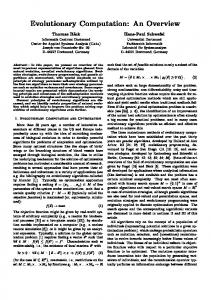
2.7 FREE OVERFALL 2.7.1 Background A free overfall is a situation where the bottom of a channel drops suddenly, causing the flow to separate and form a free nappe (Sterling and Knight, 2001). The depth of water at the section where the overfall occurs is known as the end depth (he) or brink depth (Figure (218)). Aside from its close relation to the broad crested weir, the free overfall forms the starting point in computations of the surface profile in gradually varied flows and hence has a distinct importance in hydraulic engineering (Chaudhry, 1993). In addition, based on various experiments on prismatic channels, the end depth (he) bears a unique relationship with the critical depth (hc). As there exists a unique stage-discharge relationship at the critical depth,

2-53

CHAPTER 2 – Open Channel Flow Modelling

this relationship enables the free overfall to be used as a simple flow measuring device (Sterling and Knight, 2001; Gupta et al., 1993). Van Leer (1922, 1924 cited in USBR, 2001) was probably the first who used the free overfall principle to measure flow in pipes flowing partially full. Ledoux (1924) and Rouse (1936) also realized that the end depth of flow in a rectangular channel could be used as a simple flow measuring device that requires no calibration. Since then, because of its importance and also relatively simple laboratory setup, a large number of theoretical and experimental studies have been carried out to understand the hydraulics of the end-depth problem and to determine the end-depth ratio (EDR=he/hc) in a wide range of channels.

e

Figure (2-18): A free overfall in a circular channel (Sterling and Knight, 2001). In the following sub-sections, the hydraulics of the free overfall will be initially described. The theoretical approaches for solving this problem will then be briefly explained.

2.7.2 The hydraulics of the free overfall Figure (2-19a) shows a schematic view of the pressure and velocity distributions along a channel with a free overfall. At the brink section, the pressure above and below the falling nappe is atmospheric and therefore the pressure distribution at this section differs from the hydrostatic pressure distribution. This pressure distribution has a mean pressure considerably less than the corresponding hydrostatic value. Figure (2-19b) shows the variation of streamline curvature, being finite at the free surface and zero at the channel bed. The strong vertical component of acceleration due to the gravity affects the curvature of the free nappe in the vicinity of the brink section. Since the free

2-54


surface profile is continuous, this effect is extended to a short distance upstream the brink section, causing an acceleration of the flow. This guarantees that the depth of flow at the brink section is less than critical depth. As a result, at sections upstream from the brink, the water surface curvature gradually decreases until a control section where the vertical component of acceleration is weak and the pressure is hydrostatic (Sterling and Knight, 2001; Dey, 2002b). In channels with a mild slope, the flow upstream of the brink is subcritical, becoming supercritical just before the brink section. Therefore at a short distance upstream of the brink, there is section where the pressure distribution is hydrostatic, the specific energy attains a minimum value and the depth of flow is critical. When the slope is steep and the approaching flow is supercritical, a critical section does not exist upstream of the brink (Sterling and Knight, 2001; Dey, 2002b). Furthermore, in supercritical conditions, every single disturbance creates cross-waves leading to difficulties in determining the depth of flow which makes the measurements difficult.

(a)

(b)

Figure (2-19): (a) Schematic view of a typical free overfall and the hydraulic aspects; (b) Streamline pattern of a free overfall (Dey, 2002b).

2.7.3 Problem formulation Despite the relatively simple experimental setup, the theoretical investigation of the free overfall phenomena is a complicated task. Parallel to the experimental investigations, many researchers have tried to explain the physics of the free overfall and establish an expression for the EDR for different channels by applying the governing equations and making some assumptions relating to the velocity and pressure distributions. Although providing some promising solutions, inadequacies in these studies have lead researchers to continue working

2-55


on this topic (Ozturk, 2005). The most common theoretical approaches are briefly explained in the following sections. Table (2-3) also shows some of the equations derived for EDR in rectangular, trapezoidal and circular channels. For a complete state of the art review on the free overfall, see Dey, (2002b).

2.7.3.1 Boussinesq approach

In curvilinear flow, assuming a constant acceleration normal to the direction of flow (az), the intensity of pressure, P, at any depth z is determined from the integration of the Euler’s equation, that is: −

∂ ( P + ρ gz ) = ρ az ∂z

(2-96)

As illustrated in Figure (2-19b), the streamline curvature of a free overfall varies from a finite value at the free surface to zero at the channel bed.

According to the Boussinesq

approximation (Jaeger, 1957) the variation of the streamline curvature with height above the channel bed (z) is assumed to be linear. Integrating Eq. (2-96) with this assumption, an equation for the effective mean hydrostatic pressure head (hep) is found (Dey, 2002a & b): hep = h +

U 2 d 2h kh 2 ; k = avr 3g h dx 2

(2-97)

where h is the flow depth, Uavr the mean flow velocity and g is the gravity. This equation is a suitable starting point for solving problems with small curvature at the free surface such as the free overfall (Dey, 2002b).

2.7.3.2 Energy approach

This method was first introduced by Anderson (1967) and later extended by others (e.g. Hager 1983). Normalizing the specific energy at the end section of the free overfall (Ee) and the change of free surface curvature by the critical depth (hc), using Q 2 / g = Ac3 / Tc and equating the obtained equations, it can be shown that the generalized equation of end-depth ratio (EDR) is: 6 Eˆ e − 4h%e − 3 f (h%e ) = 0

(2-98)

2-56


where Eˆ e = Ee / hc , h%e = EDR = he / hc , f (h%e ) = Ac3 /( Ae2Tc hc ) , T is the top width of flow and the subscript ‘e’ refers to the end section. It is to be further noted that in Eq. (2-98) the energy coefficient, α, is assumed to be unity.

2.7.3.3 Momentum approach

This approach is the perhaps the most popular theoretical approach towards the free overfall problem as it has been extensively applied to different channels by many researchers (e.g. Delleur et al.,1956; Diskin, 1961; Rajaratnam and Muralidhar, 1964a & b; 1970, Keller and Fong, 1989; Bhallamudi, 1994; Dey, 1998; 2001b, 2002b; 2003; Dey and Kumar, 2002). Because of the accelerated flow and the inclined streamline pattern, the pressure at the end section is non-hydrostatic (Figure (2-19a)). In this approach, a control volume is considered between a section upstream which has hydrostatic pressure, and another at the brink. Furthermore for analytical simplicity, pseudo-uniform flow (Hager and Hutter, 1984; Dey, 1998) is assumed within the control volume, where the boundary frictional resistance is compensated for by the streamwise component of the gravity force of fluid.

Hence,

considering one-dimensional momentum equations between the mentioned sections, the difference of force due to pressure will be equal to the rate of change of momentum: F0 − FP = ρ Q( βV − β 0V0 )

(2-99)

where FP is the total force due to pressure, ρ the mass density of the fluid, β the Boussinesq coefficient. Subscript ‘0’ refers to the section with hydrostatic pressure. Assuming a pressure distribution at the end section, Eq. (2-99) is solved for the EDR.

2.7.3.4 Weir approach

Assuming a zero pressure distribution and parallel streamlines at the end section and neglecting the narrowing of the nappe, the flow of a free overfall in a channel can be assumed to be similar to the flow over a sharp-crested weir having the same section with crest height equaling zero. The discharge Q of a weir is computed from:

2-57


h0

Q = Cd 2 g ∫ 2b ( H − zn ) dy

(2-100)

0

where Cd is the coefficient of discharge, b is the channel semi width at an elevation zn and H is the total head. Considering the flow at the upstream section to be critical, and substituting the total head ( H = h0 +

V02 ), Eq. (2-63) is solved for the EDR (Rouse, 1936; Ferro, 1999; 2g

Dey, 2001a & c, 2002b).

2.7.3.5 Free vortex approach

In the free vortex approach, firstly introduced by Ali and Sykes (1972), the flow at the end of a horizontal channel is simulated by the velocity distribution and curvature of a free-vortex. Expressing the discharge as the integration of the product of velocity and curvature of the free vortex, and assuming there is no loss of energy in the surface and bed streamlines, the EDR for channels with different cross sections can be derived (Dey, 2002b).

2.7.3.6 Potential flow approach

Using an iterative process, the finite difference approximations in the Laplace and Bernoulli equations for the potential flow in a free overfall are solved together with boundary conditions and the consistency of the total head and zero pressure at the free streamlines. The relaxation method (Marchi, 1993; Markland, 1965; cited in Dey, 2002b) is normally applied to solve the finite difference approximations (Southwell and Vaisey, 1943; Dey, 2002b).

2.7.3.7 Empirical approaches

In addition to the mentioned approaches, numerous researchers (e.g. Gupta et al., 1993; Pagliara, 1995; Davis et al.; 1998, Sterling and Knight, 1991; Dey, 2002b) have obtained relationships for the EDR and/or the Q by applying regression analysis on the experimental data.

2-58


2.7.3.8 Machine learning approaches

Recently, the existence of a relatively large database on the free overfall in various channels has led some researchers to apply machine learning and data modelling techniques for investigating the end-depth relationship. For example Raikar et al. (2004) used a four-layer Artificial Neural Network (ANN) model to analyze the experimental data to determine the EDR for a smooth inverted semicircular channel in all flow regimes. Ozturk (2005) used the same technique and investigated the EDR in rectangular channels with different roughnesses. Most recently, Pal and Guel (2006, 2007) applied a support vector machine (Bishop, 2006) based modelling technique to determine the EDR and discharge of a free overfall occurring over inverted smooth semi-circular channels, circular channels with flat base and also trapezoidal channels with different bed slopes.

2.7.3.9 Turbulence modelling approaches

A complete solution of the free overfall requires an integration of the turbulent Navier-Stokes equations, using an adequate turbulence model to represent the turbulent shear stresses. Many researchers have followed this approach and tried to find exact solutions for this problem. Finnie and Jeppson (1991) were perhaps among the first who stepped in this path and attempted this type of calculation for the related problem of flow under a sluice gate using the k-ε method. Mohapatra et al. (2001) also provided a numerical solution method based on the generalized simplified marker and cell (GENSMAC) flow solver and Young’s volume of fluid (Y-VOF) surface-tracking technique to the Euler equations of motion, for ideal flow past a free overfall of rectangular channels. Guo (2005) treated the free overfall in a rectangular channel by using two-dimensional steady potential flow theory. Based on the theory of the boundary value problem of analytical function and the substitution of variables, he derived the boundary integral equations in the physical plane for the free overfall in a rectangular channel. In continuation of the previous work, Guo et al. (2006) applied the volume of fluid (VOF) technique to solve the 2D incompressible RANS and continuity equations for rough rectangular channels. Ramamurthy et al. (2006) also applied the three-dimensional two-equation k-ε turbulence model together with the volume of fluid (VOF) turbulence model to obtain the pressure head distributions,

2-59


velocity distributions, and water surface profiles for the free overfall in a trapezoidal open channel. Even though the mentioned approaches yield a number of promising solutions, various inadequacies, mainly relating to the assumed distributions of velocity and/or pressure, have foreclosed the arising of a firm, suitable and general notation of the free overfall process. As it will be shown latter, an attempt will be made to use Evolutionary Computation to derive knowledge from various sources of data and to induce a global conceptual model for the free overfall which can be applied to all possible geometries and flow regimes.

2.8 CONCLUDING REMARKS It was shown that the SKM is a simple depth-averaged flow model, based on the RANS equations which can be used to estimate the lateral distributions of depth-averaged velocity and boundary shear stress for flows in straight prismatic channels with the minimum of computational effort. However, in order to apply the SKM successfully, the channel cross section should first be divided into a number domains (panels) based on an adopted panelling philosophy. Then, in addition to the inputs of cross-sectional shape and longitudinal bed slope, the correct lumped values of the friction factor (f), dimensionless eddy viscosity (λ) and a secondary flow term (Γ), for each panel should be fed to the model as inputs. Although there are some initial guidelines for the selection of the named parameters (Knight and Abril, 1996; Abril and Knight, 2004; Chlebek and Knight, 2006), their lateral variation is still unknown largely. The final section of the chapter introduced the free overfall as an effective and simple discharge measuring device. The amount of published work in the literature indicates the high attention of hydraulic engineers to this problem. However, all the applied approaches for determining the EDR or the discharge are accompanied with faults, uncertainties and lack of generality. Having introduced the above, the tools used in this research for bridging the identified knowledge gaps will be presented in the following Chapter. In Chapter 3 an attempt is made to provide a conceptual view on Evolutionary Computation and describe its application in multi-objective model calibration and symbolic regression.

2-60


Circular

Trapezoidal

Rectangular

Channel

EDR = he/hc

Channel status

Approach

Researcher

0.715

Horizontal, Smooth

Weir

Rouse (1936)

0.731

Horizontal, Smooth

Momentum

Diskin (1961)

0.649

Sloping, Smooth

Energy

Anderson (1967)

0.781

Mild slope, Roughness

Empirical

Bauer and Graf (1971)

0.678

Horizontal, Smooth

Free-vortex

Ali and Skyes (1972)

0.667

Horizontal, Smooth

Momentum

Ali and Skyes (1972)

9 F02 /(9 F02 + 4)

Sloping, Smooth

Energy

Hager (1983)

0.696

Sloping, Smooth

Momentum

Hager (1983)

0.760

Horizontal, Smooth

Momentum

Ferro (1992)

0.706

Sloping, Smooth

Free-vortex

Marchi (1993)

134.84 S02 − 12.66 S0 + 0.778

Sloping, Rough

Empirical

Davis et al. (1998)

0.848e( −0.225 F )

Sloping, Rough

Empirical

Davis et al. (1998)

0.846 − 0.219( S0 / n)0.5

Sloping, Rough

Empirical

Davis et al. (1998)

0.77 − 2.05S0 0.5

Sloping, Smooth

Empirical

Firat (2004)

0.76 − 1.29S00.5

Sloping, Rough

Empirical

Firat (2004)

0.76 − 0.02S00.5 / n

Sloping, Smooth-rough

Empirical

Firat (2004)

0.6701 − hn / hc

Sloping, Smooth-rough

Empirical

Firat (2004)

0.7016

Sloping , Smooth

Free-vortex

Beirami et al. (2006)

0.745

Horizontal

Empirical

Gupta et al. (1993)

0.7267e −5.5 S0

Sloping , Smooth

Empirical

Gupta et al. (1993)

0.705 + 0.029(mhc / B )

Horizontal

Empirical

Pagliara (1995)

0.715

Horizontal, Smooth

Momentum

Smith (1962)

0.75, (hc/d) < 0.82

Sloping , Smooth

Momentum

Dey (1998)

2 F02 /(1 + 2 F02 )) 2 / 3

Sloping , Smooth

Momentum

Clausnitzer & Hager (1997)

0.743

Sloping , Smooth

Empirical

Sterling & Knight (2001)

Table (2-3): EDR for rectangular, trapezoidal and circular channels.

2-61

CHAPTER 3 – Evolutionary and Genetic Computation

CHAPTER 3

EVOLUTIONARY AND GENETIC COMPUTATION

3.1 INTRODUCTION The aim of this chapter is to review the essential knowledge required for the implementation of the genetic algorithm and genetic programming used in subsequent chapters. The chapter starts with presenting a short history and conceptual view of Evolutionary Computation (EC) and describes the main operations used in this paradigm. Then, a simple genetic algorithm (GA) and its operators are described as a subset of EC techniques. This opening section is followed by two separate sections each dedicated to the EC approaches employed in this research. The first approach is evolutionary multi-objective (EMO) optimization for model calibration. In this section, the concepts of model parameter estimation, multi-objective optimization and Pareto optimality are explained.

Then, an EMO method named non-

dominated sort genetic algorithm II (NSGA-II) which is the primary element of the proposed calibration framework for the SKM will be examined in detail. The second approach is related to evolutionary knowledge discovery.

After providing a brief background on

knowledge discovery and explaining its processes, symbolic regression is introduced as an effective data mining tool for knowledge discovery and model induction. This section ends with a brief explanation of another EC method: Genetic Programming (GP). This technique will be used to derive a novel formulation of the physical laws of the free overfall.

3.2 EVOLUTIONARY COMPUTATION Inspired by Darwin’s theory of natural evolution and motivated by the development of computer technologies, EC was introduced in the 1960s as a robust and an adaptive search method. Simulating the natural evolutionary process, these techniques are able to look for the

3-1


best (fittest) solution(s) among an enormous number of possible candidates. In the following sections, a short history of EC, the related biological terminology and the EC process are discussed.

3.2.1 Short history of evolutionary computation Although some ideas underlying research in EC can be traced to the first half of the 20th century, the effective beginning of the field should be placed in the 1960s, concordant with the computer technology revolution (De Jong, 2006; Back et al., 1997b). Rechenberg (1965; after Bach and Shcwefel, 1993) is acknowledged as one of the pioneers in this field. In his early work, he developed an evolutionary based method for solving real-valued parameter optimization problems. The main genetic operator in the original version of this method was high level mutation (asexual alteration) and no crossover (sexual recombination) was used (see Section 3.2.2 for terminology). His work was the building block of a method which is today called Evolution Strategy (ES). Two other main streams which emerged from the basic idea of EC can be identified as Evolutionary Programming (EP), originally developed by Fogel, Owens and Walsh (1966) and Genetic Algorithms (GAs) by Holland (1962, 1975). Compared to ES, EP used a more flexible representation and was applied to evolve finite state machines to solve various problems. In the milestone book of “Adaptation in natural and artificial systems” Holland (1975) introduced ECs (particularly genetic algorithms) as a robust method of nonlinear optimization. This approach introduced the crossover operator and used binary strings as representation.

Overcoming the methodological shortcomings and the advent of powerful computational platforms during the 1980s enabled EC to solve difficult real-world problems (Back et al., 1997b). This attracted the research community and resulted in the combination, refinement and modification of the main stream. As a result, by the early 1990s, the word “Evolutionary Computation” started to appear in the scientific terminology. More than thirty years of practical application of EC in different fields has demonstrated that this paradigm is capable of dealing with a large variety of problems (Back and Shcwefel, 1993). Nevertheless, the current state of knowledge is still far behind the real concept of evolution in the natural life

3-2


which makes the field of EC an exciting one for further scientific applications (Nazemi, 2008).

3.2.2 Biological Terminology Since natural biological evolution is the basis of EC, it is essential to understand its basic terminologies and discovered rules. The main principle of Darwinian evolution is “survival of the fittest”, i.e. only highly fit organisms will be able to survive and reproduce in their environments (Mitchell, 1999). To be more concise, evolution can be defined as a long time scale process that changes a population of organism by generating better offsprings through reproduction. The basic terminologies of biological evolution, which are commonly used in the context of EC, can be summarized as follows:

Chromosomes:

are strings of coiled DNA that contain the coded characterization information of an organism. A chromosome can be conceptually divided into genes.

Genes:

are elementary blocks of information in the DNA structure which encode a particular protein (e.g. eye colour).

Traits:

are the physical characteristic encoded by a gene (e.g. eye colour, hair colour…).

Alleles:

are the different possible settings for a trait (e.g. brown, blue . . .).

Locus:

is the location of a gene on the chromosome.

Genome:

is the complete collection of all chromosomes in an organism's cell.

Genotype:

is a particular set of genes contained in a genome.

Phenotype:

Is the physical and mental realization of a genotype (e.g. height, brain size, and intelligence).

Fitness:

is the probability that the organism will live to reproduce (viability) or the number of offspring the organism has (fertility).

Crossover:

is a genetic operator where chromosomes from the parents exchange genetic materials to generate a new offspring.

Mutation:

is the error occurring during DNA replication from parents.

3-3


3.2.3 Evolutionary computation process Conceptually, all EC methods are based on initializing a population of potential candidates (Chromosomes) using a coding scheme, evaluating each individual within the population and giving fitter solutions more chance to evolve and pass through next generations. In the search for the best solution, evolution tries to gradually improve the quality of individuals by selecting, recombining (crossover) and altering (mutation) the fittest individuals. This general procedure can be algorithmically shown in the form of a “pseudo-code” (Michalewicz, 1996): t := 0; code [problem representation] initialize [Pt] evaluate [Pt]

while not terminate do Qt := variation [Pt] evaluate [Qt]

Pt+1 := select [Pt ∪ Qt] t := t + 1 End while In this algorithm, Pt denotes a population of individuals at generation t and Qt is the offspring population created from the evolution of selected population individuals by means of variation operators such as recombination and mutation. Any algorithm that adopts this general structure is called an Evolutionary Algorithm (EA).

3.2.4 Evolutionary Algorithms (EAs) Recalling the general EC procedure, an EA must have the following four basic components (Michalewicz, 1992): 1- an evolutionary representation of the solutions to the problem, 2- a way to create an initial random pool of candidate solutions, 3- an evaluation function for rating solutions in terms of their “fitness” and 4- genetic operators that evolve the population towards fitter solutions during reproduction.

3-4


Obviously, the distinction between different types of EAs lies in variations in the named key elements. Figure (3-1) shows the common classification of EAs based on their semantic. This family encompasses five members: Evolution Strategies (ES): Developed by Rechenberg (1965), this method adopts vectors of real numbers as representations, and typically uses self-adaptive mutation rates to solve optimization problems. Evolutionary Programming (EP): This technique was pioneered by Fogel, Owens and Walsh (1966) to develop artificial intelligence. In contrast to other more adopted EAs, in EP no exchange of material between individuals in the population is made. The developed versions of this method are used for solving general tasks including prediction problems, optimization, and machine learning. Genetic Algorithm (GA): Introduced by Holland (1975), GA is perhaps the most popular type of EA. GA seeks the solution of a problem in the form of strings of numbers (traditionally binary) by applying recombination operators in addition to selection and mutation. This type of EA is often used in optimization problems (see Section 3.2.5 for more details). Learning Classifier Systems (LCS): LCS are rule-based systems that are able to automatically build the ruleset they manipulate. They were invented by Holland (1975) in order to “model the emergence of cognition based on adaptive mechanisms” (Sigaud and Wilson, 2007). Genetic Programming (GP): GP was introduced by Koza (1990; 1992) with the aim of allowing computers to solve problems automatically by evolving computer programs. The representations which evolve through the generation are structures of programs or expressions. GP is used in solving many types of problems in the field of artificial intelligence (see Section 3.4.4 for more details).

3-5


Figure (3-1): The family of evolutionary algorithms (Weise, 2009).

The recombination and mutation operators used in most EAs have made them successful in solving a wide variety of problems. Furthermore, due to the stochastic nature of these methods, no gradient or special knowledge is usually required about the problem. This flexibility has allowed EAs to be successfully applied to multimodal, complex problems where most traditional methods are largely unsuccessful (Deb, 1997). However, like other traditional search and optimization methods, there are some drawbacks in using EAs. One major limitation emerges from the improper choice of EA parameters such as population size, crossover and mutation probability. In order to successfully apply an EA to a problem, the user must be aware of the proper choices for the parameters as these methods may not work efficiently with an arbitrary parameter setting. Another problem in using EAs is that since most of the operators are based on random generated numbers, the overall performance largely depends on the chosen random number generator. Hence, an unbiased random number generator must be used to preserve the stochasticity in the operators and ensure the correctness of the results. The total computational effort is another drawback of EAs. Since generally no gradient information, or problem knowledge is used, compared to classical search methods, EAs may require more function evaluations for simple, differentiable, unimodal functions (Deb, 1997).

In addition to main categories of EAs, there are also many hybrid approaches which incorporate various features of the evolutionary paradigm, and consequently are hard to classify (Michalewicz, 1996). The detailed description of different EAs is far beyond the

3-6


scope of this thesis. However, GA and GP which are incorporated in this research will be described in more detail in what follows.

3.2.5 Simple Genetic Algorithms (GA) A simple Genetic Algorithm (GA) has been adopted as the representative of EA for two reasons. Firstly, it is relatively easy to understand and can be briefly explained and secondly, it contains all the genetic-based processes which are incorporated in the more sophisticated EA approaches. In the following sections, a brief background of simple GA and its elements are provided. For detailed explanation and history the reader is referred to Holland (1975), Goldberg (1989), Koza (1992), Coley (1999) and Osyczka (2002).

3.2.5.1 Background Inspired by evolutionary biology, John Holland invented GAs in the 1960s with the goal of developing search methods for importing the mechanisms of natural adaptation into computer systems.

His ingenious idea was further developed by him and his co-workers at the

University of Michigan in the 1960s and the 1970s. Their findings were published in 1975 under the title of “Adaptation in Natural and Artificial Systems”. The book presented the genetic algorithm as an abstraction of biological evolution and provided a theoretical framework for EC.

Genetic algorithms have undergone several modifications since their introduction, which have made them capable of solving many large complex problems. The main characteristics of these techniques that have made them popular for scientists and engineers are (Coley, 1999):

1- their ability to tackle search spaces with many local optima. 2- their ability to estimate many parameters that interact in highly non-linear ways. 3- their ability to deal with non-continues search spaces. 4- they are generally insensitive to initial conditions. 5- they are more efficient at locating a global peak than traditional techniques.

3-7


These abilities have resulted in an excellent reputation that has led GA to be successfully applied to problems where other methods have experienced difficulties. Acoustics and signal processing (Sato et al., 2002), Aerospace engineering (Obayashi et al., 2000), Astronomy (Charbonneau, 1995), Chemistry (Gillet et al., 2002), Financial marketing (Andreou et al., 2002) Game playing (Chellapilla and Fogel, 2001), Geophysics (Sambridge and Gallagher, 1993), Material engineering (Giro et al., 2002), Medicine (Yardimci, 2007) and Water engineering (Bekele, 2007) are among the many fields which GAs have been successfully applied to.

3.2.5.2 Representation In GA, the search starts with an initial set of random candidate solutions represented as chromosomes. Each chromosome consists of genes which stand for a particular element (e.g. a parameter in a multi-variable optimization problem) of the candidate solution. Simple GA uses binary coding where the genes are formed of bit strings of 0’s and 1’s. Figure (3-2) shows a chromosome with 5 genes, each representing a parameter of a potential solution. This chromosome is equivalent to the parameter set of {5,7,5,3,11}. The main drawback with this coding is that it requires long chromosomes to represent all the potential solutions in large search domains. This will result in the requirement of more memory and processing power.

Figure (3-2): A chromosome with 5 genes.

The main alternatives to binary-coding are Gray coding (Caruana and Schaffer, 1988), fuzzy coding (Sharma and Irwin, 2003) and real number coding (Deb and Kumar, 1995). In real number coding, which is incorporated in this thesis, real numbers are used to form a chromosome-like structure for the decision variable. This enables the assignment of large domains (even unknown domains) for variables (Deb and Kumar, 1998). For an in-depth review on different EA representations see Rothlauf (2006).

3-8


3.2.5.3 Genetic Algorithm process The general GA process can be summarized as continuously moving from one population of candidate solutions (chromosomes) to a new population of fitter solutions by using a kind of natural selection together with the genetic operators of crossover and mutation. This cycle of evaluation – selection – reproduction is continued until an optimal or a near-optimal solution is found (Goldberg, 1989; Michaelwicz, 1992). Figure (3-3) illustrates the flow chart of a simple GA process.

Once the initial population is generated, each chromosome is evaluated and its “goodness” (fitness) is measured using some measure of fitness function. Then, based on the value of this fitness function, a set of chromosomes is selected for breeding. In order to simulate a new generation, genetic operators such as crossover and mutation are applied to the selected parents. The offsprings are evaluated and the members of the next generation population are selected from the set of parents and offsprings. This cycle continues until the termination criterion is met. START

Encoding

New Population

Initial population generation

Evaluation Selection

Crossover

Mutation

Generate new offsprings

Selection

NO

Evaluation

Decoding

Termination ? YES

STOP

Figure (3-3): Process of simple Genetic Algorithm.

3-9


3.2.5.4 Initialization In simple GA, the process of initialization involves the random production of a set of binary strings.

The only internal parameter in this process is the population size (number of

chromosomes).

It has been shown (Lobo, 2000) that the population size can have an

important role in the evolutionary search and therefore has to be considered carefully. If the population size is too small, the diversity in the population is too low and the population will soon suffer from premature convergence. On the other hand, if the size is too large the convergence towards the global optimum is slow and requires large computation resources.

3.2.5.5 Evaluation (measuring performance) Fitness is the driving force of Darwinian natural selection (Koza, 1990) and the performance measure is the main feedback to an evolutionary algorithm. Selection of a performance measure clearly depends on the kind of task and desired characteristics of the discovered solution. A good performance measure should be able to give a fine-grained differentiation between competing solutions, focus on the eventual use of the program and avoid giving false information (Keijzer, 2002). One common fitness function is the sum of the squared distances between the value returned by the individual chromosome and the corresponding observed value. Using this fitness function for measuring the fitness increases the influence of more distant points. Obviously, the closer this sum of distances is to zero, the better the individual.

3.2.5.6 Selection The selection operator chooses those chromosomes in the population that will be allowed to reproduce and also the individuals that will be passed to the next generation. As a result of this natural selection, better performing (fitter) individuals would have a greater than average chance of reproducing and promoting the information they contain to the next generation. The three most commonly used selection schemes are proportionate selection, rank selection, and tournament selection (Goldberg and Deb, 1991). In proportionate selection, also known as “roulette wheel” selection, the likelihood of selecting a chromosome is equal to the ratio of the fitness of the chromosome to the sum of the fitness of all chromosomes. One serious limitation of this method is that one comparatively very fit chromosome can very quickly overcome a population.

Rank and tournament selection are designed to overcome this

3-10


problem. In rank selection, the population is sorted from best to worst fitness, and the probability of selection is some (linear or nonlinear) function of rank.

In tournament

selection, some small number of chromosomes (frequently two) are chosen at random, compared, and the fittest chromosome is selected; this process is repeated until sufficient chromosomes have been selected.

For an authorative study on selection methods, see

Goldberg and Deb (1991).

3.2.5.7 Crossover Crossover has been cited as the main genetic operator of GA and other EC techniques (e.g. Colley 1999; Osyczka, 2002). This operator allows solutions to exchange information in a way similar to that used by a natural organism undergoing reproduction. There are many ways to perform crossover (Michalewicz, 1992).

The simplest method is single point

crossover, where the chromosomes are split at a randomly selected point, and genes to the left of the split from one chromosome are exchanged with genes to the right of the split from the other chromosome, and vice versa (Figure (3-4)). The effect of crossover is controlled by crossover rate (probability) which defines the ratio of the number of offspring produced in each generation based on crossover. It has been shown (Lobo, 2000) that the crossover rate can have a major effect on the quality of evolutionary search. A higher crossover rate allows exploration of more of the solution space and reduces the chances of getting trapped in local optima. On the other hand, a very high crossover rate can result in unnecessary searches in unpromising regions.

Figure (3-4): Single point binary crossover operator.

3-11


3.2.5.8 Mutation Mutation is another genetic operator which introduces extra diversity in the population by making “accidental” changes in randomly chosen chromosomes. This will ensure the search of the entire solution space over the course of the entire evolution (Michalewicz, 1992). In its simplest version, this operator randomly changes the value of single bits within individual strings to keep the diversity of a population and to help a genetic algorithm get out of a local optimum (Figure (3-5)). Like crossover, the contribution of mutation in evolutionary search is controlled by the so-called mutation rate (probability) which has certain influence on the evolutionary search. If the mutation rate is too high, then the offspring will lose their relationship with their parents (Back et al., 1997a). That means the resulting generation forgets the history of evolution.

Figure (3-5): Binary mutation operator.

3.2.5.9 Termination The evolutionary cycle of evaluation-selection-reproduction continues until a stopping criterion is met. The easiest and most common termination criterion is the maximum number of generations, which is the one that has been incorporated in this thesis. Other stopping criteria which have been used in literature include: •

Stopping after a maximum number of function evaluations.

•

Stopping after a predefined fitness has been achieved.

•

Stopping when the rate of fitness improvement slows to a predefined level.

•

Stopping when the population has converged to a single solution.

3-12


3.3 EVOLUTIONARY MULTI-OBJECTIVE MODEL CALIBRATION 3.3.1 Model parameter estimation (model calibration) Environmental models are “lumped approximations of the heterogeneous world” (Wagner and Gupta, 2005).

These models attempt to represent the complex, spatially distributed,

interactions of earth, water, vegetation and energy by means of combining the physical laws of conservation and the physical properties of the system (Wagner and Gupta, 2005). Inevitably, there are always a number of parameters in the system whose values, mainly due to “immeasurability”, are not known precisely. This immeasurability is down to the lack of an exact physical interpretation of the parameters (e.g. friction factor (see Section 2.6.7)) and/or measurement techniques (e.g. eddy viscosity (Section 2.6.8) and secondary flow term (Section 2.6.9)). Therefore, before a model can be used to simulate the real-world processes, the values of some of its parameters should be adjusted. This process is best known as parameter estimation or model calibration, and will result in finding the “optimal” values of the immeasurable parameters in the model.

The objective of parameter estimation is to calibrate the model so that the observed and calculated system responses show a significantly high degree of similarity (Wagner et al., 2003). Gupta et al. (2005) define three necessary conditions for an environmental model to be “well-calibrated”:

1- The input–state–output behaviour of the model is consistent with the measurements of the system behaviour. 2- The model predictions are accurate (i.e. they have negligible bias) and precise (i.e. the prediction uncertainty is relatively small). 3- The model structure and behaviour are consistent with a current environmental understanding of reality.

The process of model calibration is normally performed either manually or by using computer-based automatic procedures.

Manual calibration is a trial-and-error procedure,

which the modeller uses a number of different measures of performance and visual inspection of the model output to define the optimum parameter values (Gupta et al., 1998). This

3-13


procedure might yield good results in simpler models but is generally very labour-intensive, time consuming, and requires considerable experience with a specific model structure. Furthermore, it is less successful in complex models where a high number of non-linearly interacting parameters are present in the model and also an objective analysis of parameter uncertainty is not possible in this procedure (Wagener et al., 2003; Cheng et al., 2006).

As a result, a significant amount of research has been directed towards the development of automatic calibration procedures. An automatic approach uses a computer algorithm to search the parameter space, performing multiple trials of the model. The performance of the model in each trial is specified by one or many objective functions. The failure of traditional automatic procedures like gradient-based methods and linear and dynamic programming techniques in solving problems with large number of variables and non-linear objective functions has contributed to the development of alternative solutions. Evolutionary based optimization algorithms such as genetic algorithms (e.g. Wang, 1991; Yapo et al., 1998), shuffled complex evolution (SCE) algorithm (Duan et al., 1992; Madsen, 2000) and simulated annealing (Sumner et al., 1997) have been extensively used as powerful global optimization tools.

3.3.2 Multi-objective optimization problem Many practical problems involve multiple measures of performance, or objectives, which are competing or conflicting and need to be optimized simultaneously. Simple examples are maximizing profit and minimizing the cost of a product and maximizing performance and minimizing fuel consumption of a vehicle. The concept of optimizing multiple, but equally important, objectives was originally introduced by two economists, Edgeworth (1881) and Pareto (1897).

The general form of a multi-objective optimization problem can be defined as the minimization or maximization of a vector of objectives, F( X ) , according to certain criteria: min or max F( X ) = { f1 ( X ), f 2 ( X ),..., f M ( X )}

(3-1)

subject to: g ( X ) ≤ 0 and

h( X ) = 0

3-14


where X = ( x1 , x2 ,..., xN ) is the decision variables vector in the domain search space, Ω, and f1 ( X ), f 2 ( X ),..., f M ( X ) are M objective functions that are to be minimized or maximized. Furthermore, g ( X ) ≤ 0 and h( X ) = 0 are inequality and equality constraints representing the majority of practical and physical constraints arising in engineering problems (Farina, 2001). Accordingly, two subspaces known as the feasible design domain search space, Ω, and the objective domain search space, Ω0 , are defined as:

{

}

Ω : X ∈ R N s.t. g ( X ) ≤ 0 and h( X ) = 0

{

}

Ω0 : F( X ) ∈ R M s.t. X ∈ Ω

(3-2)

(3-3)

Where R is the set of real numbers and Ω0 is the image of Ω through function F. It should be noted that based on the nature of the problem, the design variables may not always belong to R N .

In contrast to single objective optimization problems, multi-objective optimization problems may not have a single solution which simultaneously satisfies all objectives to the same extent. In fact there exists a set of equally good optimum solutions (trade-offs) none of which without any further preference information, can be said to be better than the others. A variety of methods exist to solve multi-objective problems. The traditional methods convert multiobjective optimization problems into a series of equivalent single-objective problems and try to find the optimum solutions with conventional techniques (e.g. linear programming, gradient methods). The most frequently adopted methods and their limitations are listed below:

1- In certain cases, objective functions may be optimized separately from each other and an insight gained concerning the “best” that can be achieved in each performance dimension. Applying this method, suitable solutions to the overall problem can seldom be found. The optimal performance according to one objective, if such an optimum exists, often implies unacceptably low performance in one or more of the other objective dimensions (Fonseca and Fleming, 1995).

3-15


2- Aggregating approaches are methods which assign weights to each objective and then re-formulate a single-objective by adding the weighted objectives and find the optimum of the new objective. These methods tend not to lead to a suitable solution as the decision regarding the “best” solution relies on the so called human decision-maker (Ghosh and Dehuri, 2004). 3- In the ε-constrained method (Hirschen and Schafer, 2006) one of the objectives is selected as the main objective and the other objectives are imposed as constraints to the problem.

3.3.3 The concept of Pareto optimality Generally, when multiple solutions of a given multi-objective problem are available, in order to distinguish between different solutions, it is necessary to rank them according to an order criterion. Based on the Pareto optima theory (Goldberg, 1989), the solutions are ranked according to the Pareto dominance concept which is defined as: For any two solutions X 1 and X 2 ∈ Ω , and assuming a minimization problem, X 1 dominates solution X 2 if: fi ( X 1 ) ≤ fi ( X 2 ) for all i ∈ [1, 2,...M ]

(3-4)

f j ( X 1 ) < f j ( X 2 ) for at least one j ∈ [1, 2,...M ]

(3-5)

In other words, if solution X 1 is not worse than X 2 in all objectives, but is strictly better in at least one objective, then it is said that X 1 dominates X 2 . Figure (3-6) illustrates a set of solutions for a typical two-objective problem where the goal is to minimize both objectives. The horizontal and vertical axes represent the value of the first and second objective respectively and each circle represents a decision vector (Xi) in the objective space ( Ω0 ). Based on the Pareto dominance concept, all empty circles are dominated by the filled ones. The union of all non-dominated solutions (filled circles) is called the Pareto set and its image in the Ωο, is known as the Pareto-optimal front. In fact the Pareto front represents best compromise solutions for which none has any precedence over any other. Once the Pareto

3-16


front of a problem is found, the engineer is able to choose the best compromise solution according to the user’s preferences.

f2(X)

f1(X)

Figure (3-6): The Pareto front of a two objective optimization problem.

Although being relatively simple, at their best, traditional optimization techniques are only able to find one solution on the Pareto front at each run, i.e. for each equivalent single objective problem being solved. Hence, they are not convenient for solving a multi-objective problem.

3.3.4 Evolutionary multi-objective optimization (EMO) Since EC methods deal with a population of solutions, it can be expected that these search algorithms can have a great potential in the discovery of Pareto optimal solutions. In addition, because of their nature, evolutionary algorithms are less susceptible to the shape and continuity of the Pareto front; the weakness of most search methods. Therefore, EMOs have the ability to handle complex problems, involving features such as discontinuities, multimodality and disjoint feasible spaces (Fonseca and Fleming, 1995). These are the features that make them suitable for solving complex multi-objective problems.

The first design of a multi-objective evolutionary algorithm (MOEA) was undertaken in the mid-1980s by Schaffer (1984).

Schaffer’s approach, called Vector Evaluated Genetic

Algorithm (VEGA) consisted of a simple genetic algorithm with a modified selection mechanism. After VEGA, several researchers have proposed other MOEAs which over the years have been used in many applications and their performances have been tested in several comparative studies. There are two common goals in all MOEA implementations. First, to

3-17


move the population toward the Pareto optimal front and second, to maintain diversity in the population so that multiple solutions can be developed (Deb, 1999). A detailed description of these algorithms is beyond the scope of this thesis. For an excellent comprehensive survey on EMO the reader is directed towards Coello (2006). Among these algorithms only the Nondominated Sorting Genetic Algorithm-II (NSGA-II), the primary element of the proposed calibration framework of the SKM, will be considered in more detail.

3.3.5 Non-dominated Sorting Genetic Algorithm-II (NSGA-II) The Non-dominated Sorting Genetic Algorithm II (NSGA-II) is a fast and elitist, second generation MOEA proposed by Deb et al. (2000; 2002). The main features of this method are:

1- at each generation, the best solutions found are preserved and included in the following generation using an elite-preserving operator; 2- a fast algorithm is used to sort the non-dominated fronts; 3- a two level ranking method is used to assign the effective fitness of solutions during the selection process. Figure (3-7) illustrates the general procedure of this method. In this figure, Pt is the parent population, Qt is the offspring population, Rt is the combined population ( Rt = Pt U Qt ) and Fi are the non-dominated sorted fronts of Rt. The algorithm starts with a random population and generates the children using the genetic operators. Then, a fast non-domination sorting algorithm is used to rank the solutions according to their dominance rank and organize fronts of equal rank.

In this ranking method, an individual, k, is randomly chosen from the

population Rt and inserted in an intermediate set named F1. Then, another solution k΄ is drawn from Rt and compared to all individuals from F1. If k΄ dominates k, k΄ enters F1 and k is deleted, but if k dominates k΄, then k΄ is deleted and k stays in F1. Continuing this comparison for all individuals, F1 will consist of all non-dominated individuals of Rt, the Pareto front by definition. Now the first Pareto front is removed from the original population

3-18


and the same procedure is iteratively continued to identify other layers of Pareto fronts { Fi , i = 1,...} . Crowding distance sorting

Non-dominated sorting

Pt + 1

F1 F2

Pt

F3

Qt

Rejected

Rt

Figure (3-7): Procedure of NSGA-II (Deb et al., 2002)

Subsequently, individual solutions within each front are ranked according to a density measure using the crowding operator. This operator, as pictured in Figure (3-8), measures the diversity of each individual by measuring half of the perimeter of the rectangle that encloses a solution in the objective function space and assigning infinite distance to the extreme points of the Pareto-front. This operator is designed in a way to ensure the selection of those individuals which reside in less crowded regions of the objective space. This will guarantee a spread along the Pareto and prevent the algorithm focusing solely on a certain part of the front.

k-1

f2(X)

k

k+1

f1(X)

Figure (3-8): Distance assignment in NSGA-II (Hirschen & Schafer, 2006).

3-19


The next generation, Pt+1, which has the same size as the first generation is filled with consecutive Pareto fronts { Fi , i = 1,...} , until no full Pareto front can be fully accommodated anymore.

Then, the solutions in the next Pareto layer are sorted in descending order

according to their distance assignment and the empty spaces in the proceeding generation are filled with higher ranked solutions. The next offspring population, Qt+1, is created by using the crowded tournament selection operator.

Two attributes can be considered for each individual solution: First, a non-

domination rank (equal to the Pareto layer rank) and second, a crowding distance (as explained beforehand).

In the tournament selection, competitions are set up between

individuals. The tournament is “won” by that individual which has the better non-dominated rank (lies on an outer Pareto front). If both individuals are on the same Pareto front, ties are broken by the crowded distance and the tournament is “won” by the one which is least crowded (Hirschen & Schafer, 2006). The procedure outlined in Figure (3-7) is repeated until the termination criterion is met and the best-known Pareto front is saved in an archive. The solutions in this archive are the Pareto optimal solutions of the problem under consideration. For an in-depth explanation of this method the reader is referred to Deb et al. (2000; 2002). Studying a variety of test cases (e.g. Deb et al. 2002; Khare et al., 2003), it has been shown that compared to other elitist multi-objective evolutionary algorithms, NSGA-II has a better diversity preservation and therefore is able to compete with them regarding to its convergence to the true Pareto-optimal front in both constraint and non-constraint problems (Nazemi et al., 2006). This superiority has lead to the successful application of NSGA-II in several real world problems such as long-term groundwater monitoring design (Reed et al, 2007), water distribution network design (Babayan et al., 2005), calibrating hydrological models (Bekele, and Nicklow, 2007; Liu et al., 2005), traffic signal timing optimization (Sun et al., 2003) and medicine (Lahanas et al., 2003).

3-20


3.4 EVOLUTIONARY KNOWLEDGE DISCOVERY 3.4.1 Background Early observations of the world through quantitative and numerical data by mankind can be dated as far back as 3500 B.C. (Powell, 1995).

Although these observations and

measurements were apparently taken for purposes other than for scientific laws, they formed the initial foundation for the development of classical science. Generally, when a set of observations of the physical system is collected, classical science attempts to describe the behaviour of the system by generating a hypothesis that represents a generalization of the data (Keijzer, 2002), whereas modern science gives a more refined and coherent representation of the physical and conceptual processes in the form of equations in a physical symbol structure (Babovic and Abbott, 1997a). Once the formulation of a scientific law or theory is obtained, additional justification is provided by finding a proper conceptualization of the problem.

Modern experimental and observational methods generate enormous datasets and the amount of data stored in databases continues to grow rapidly. These large databases can contain valuable hidden knowledge, which, if extracted, can be used to improve the understanding of real-world processes. The amount of stored data grows at a much larger rate than the number of human data analysts. Hence, there is a need for (semi-)automatic methods to assist the human analyst in extracting knowledge from data. This need has led to the emergence of a field known as Knowledge Discovery (Freitas, 2002). This is an interdisciplinary field where methods of several research areas such as Machine Learning and Statistics are used to extract high level knowledge from real-world datasets. Knowledge Discovery has Data Mining as its heart and also consists of several pre-processing methods aimed at facilitating the application of the data mining algorithm, and post-processing methods to refine and improve the discovered knowledge (Freitas, 2002).

The discovered knowledge, as stated by Freitas

(2002), should satisfy three general properties: it should be accurate, comprehensible and interesting.

3-21


3.4.2 Knowledge discovery process As stated above, the Knowledge Discovery process consists of three main distinctive stages: data preprocessing, data mining and discovered-knowledge post-processing (Freitas, 2002). All the tools used in this process, facilitate the conversion of data into a number of forms that convey a better understanding of the process that generated or produced these data (Keijzer, 2002). Figure (3-9) illustrates an overview of the entire Knowledge Discovery process. The directions of the arrows in the Figure indicate that this process is inherently iterative, i.e. the output of a step can either be sent to the next step in the process, or be sent back to a previous step as a feedback (Freitas, 2002).

Figure (3-9): An overview of the Knowledge Discovery process (Freitas, 2002).

3.4.2.1 Data preprocessing

Data preprocessing (or data preparation) is the first stage of Knowledge Discovery where the data are cleaned and transformed to ensure accurate and efficient results. The following procedures may be performed in this procedure (Pyle, 1999): a) Data Integration: If the data come from different sources, such as several departments of

an organization or various research papers, it becomes necessary to integrate all the data in one suitable format. This involves tasks such as removing inconsistencies in attribute names or values between data sets of different sources.

3-22


b) Data Cleaning: It is important to make sure that the data are as accurate as possible. This

step may involve detecting and correcting errors in the data, filling in missing values, etc. Some data cleaning methods for data mining are discussed in Guyon et al. (1996) and Simoudis et al. (1996). c) Discretization: This step is particularly required when the data mining algorithm cannot

handle continuous attributes. For this purpose, continuous attributes are transformed into a categorical (or nominal) attribute which only take a few discrete values. For instance the realvalued attribute “uncertainty” can be discretized to undertake only three values: low, medium and high. d) Attribute Selection: As indicated by its name, this step comprises selecting a subset of

attributes among all original attributes, which are relevant for the Knowledge Discovery process.

3.4.2.2 Data mining

Data Mining is defined as the (semi-)automatic extraction of interesting knowledge from data and is considered as the core step of the Knowledge Discovery process. Some problems which can be solved by data mining algorithms are: classification, dependence modelling, clustering, discovery of association rules and model induction problems. In the context of this research, the favourable application of data mining is model induction where the main objective is to deduce a closed-form explanation of the system based solely on observations. In this approach, the modeller uses the data mining techniques in an attempt to drive a complete model from the limited information of the physical system that can account for both the entire range of observed and unobserved phenomena within the physical system. The important point about this type of modelling is, as Keijzer (2002) states, “the confidence in model performance cannot be based on data alone, but might be achieved by grounding models in the domain so that appropriate semantic content is obtainable”. As a result, the

obtained models can be used to reinforce, inspire or abandon the scientists’ view of the problem (Keijzer, 2002).

3-23


3.4.2.3 Post-processing stage

After applying the data mining algorithm to the processed data, the discovered knowledge normally needs to undergo some post-processing treatment to improve its comprehensibility and/or interestingness. Using his interpretation, analysis and available understanding of the physical processes, the modeller plays a pivotal role at this stage by extracting a subset of “interesting” patterns of knowledge (models) (Keijzer, 2002). It is argued (Silberschatz and Tuzhilin, 1996) that in many applications, a different notation of “interestingness” is required, however, novelty, simplicity, implicity, validity on test data and potential usefulness are the general attributes of an interesting pattern (Ghosh and Jain, 2005).

Methods for the selection of interesting models can be divided into subjective and objective methods (Freitas, 1998; 1999; Ghosh and Jain, 2005). Subjective methods are user-driven and domain-dependent whereas objective methods are data-driven and domain-independent. The most common subjective approach is specifying model templates, i.e. the modeller can set rules to indicate which combination of attributes must occur in the model for it to be considered interesting (Klemettinen et al., 1994). By contrast, in objective approaches the discovered models are compared with each other with respect to their performance and not the modeller’s beliefs. Some objective measures of model interestingness are discussed in Freitas (1998; 1999). It is generally believed that in order to find interesting knowledge, an ideal combination of subjective and objective approaches should be used in the post-processing stage.

3.4.3 Evolutionary symbolic regression The most practised method of empirical model induction is deriving the relation between the variables of a system in a symbolic form (equation) by regression analysis. In the process of traditional regression (e.g. simple linear, polynomial, Fourier, etc.), the functional structure between dependent variables is predefined, and the goal is to discover a set of numerical coefficients which minimize a measure of performance between the observed and computed values of the dependent variable(s). If X = ( x1 , x2 ,..., xn ) is the set of independent input variables and Y is the desired dependent output variables of a system, the regression task is to search the potential search space and approximate Y using X and coefficients c such that:

3-24


Y = f ( X , c) + ε n

(3-6)

where ε n represents a noise term. With standard regression techniques the functional form f is pre-specified. Using linear regression for example, f would be: f ( X , c) = c0 + c1 x1 + ... + cn xn

(3-7)

where the coefficients c are found using an optimization method e.g. least square regression. For complex and unknown systems, a predefined structure may not give a fit that appeals to the eye and even if it does, the model might not necessarily make much sense from the physical point of view. In contrast to the traditional methods, symbolic regression methods (Keijzer, 2002) discover both the correct functional form that fits the data and the appropriate related numeric coefficients (Koza, 1990). This has made them a popular tool for data mining and solving model induction and empirical discovery problems (Langley and Zytkow, 1989). Symbolic regression methods include any method of inducing a symbolic description from the observed data of a system, by searching a space of potential solutions. Genetic Programming (GP) (Koza, 1990; Koza, 1992), Grammar Evolution (GE) (Ryan et al., 1998) and Analytic Programming (AP) (Zelinka et al., 2005) are the most famous symbolic regression techniques. In the following section, Genetic Programming will be introduced as an effective evolutionary data mining tool for symbolic regression and model induction.

3.4.4 Genetic Programming (GP) Genetic programming (Koza, 1990; Koza, 1992) is a collection of EC techniques based on the principles of Darwin’s theory of evolution, that allow computers to solve problems automatically by evolving computer programs (Poli et al., 2008). GP was first introduced by Koza (1990) as a powerful tool for solving problems in various fields of artificial intelligence. Starting with a number of random solutions, this technique is able to tackle any problem which can be viewed as a problem of discovering a computer program by improving the quality of the solutions by means of some natural variation operators. These problems can be categorized as symbolic function identification, symbolic regression, empirical discovery, symbolic “data to function” integration and symbolic “data to function” differentiation, solving functional equations, machine learning of a function, planning in artificial intelligence and robotics, automatic programming, pattern recognition and game playing (Koza, 1990).

3-25


In the context of Knowledge Discovery and model induction, a distinct advantage of GP over other modelling techniques such as artificial neural networks is that the provided answer in the form of a symbolic expression is in a language the user understands and can be interpreted by scientists (Keijzer and Babovic, 1999). This mathematical representation provides a great benefit in empirical modelling of unknown phenomena where an underlying theoretical model does not exist (Keijzer, 2002). This has resulted in the successful application of GP to a wide range of practical problems over the last two decades. Image and signal processing (Marko and Hampo, 1992), industrial process control (Castillo et al., 2006), medicine and bioinformatics (Koza and Andre, 1996) and economic modelling (Chen and Liao, 2005) are just a small number of problems which have been tackled by GP.

3.4.4.1 Overview

Being from the family of genetic-evolutionary techniques, GP follows a similar procedure as genetic algorithms (GAs). The standard GP starts with an initial population of randomly generated symbolic expressions (also known as parse trees) composed of functions and terminals appropriate to the problem domain. These functions may be standard arithmetic operations (such as addition, subtraction, multiplication, and division), standard mathematical functions (such as SIN, EXP, etc.), standard programming operations (such as If-Then-Else, Do-Until, etc.), Boolean functions (such as, AND, OR, XOR, NOT, etc.) and various domainspecific functions (Koza, 1990). The terminals may be variable arguments, such as the attributes of the system, constant arguments, such as 0 and 1 or a random generated number.

A fitness function is then used to measure the performance of each individual symbolic expression in the particular problem environment. Predictably, the majority of the initial random symbolic expressions have exceedingly poor fitnesses but nonetheless, some individuals are more fit than others. Then, a sexual genetic reproduction process is performed on pairs of expressions, which are selected in proportion to their fitness, and offsprings are created. The resulting offsprings are composed of sub-expressions (also known as building blocks) from their parents and form the new generation which replaces the old population of parents. The fitness function is again used to measure the fitness of each individual in the new population. Repeating this algorithm will gradually produce populations which, over a period of generations, reach a high average fitness in dealing with their environment. Figure

3-26


(3-10) shows the flowchart of the computational procedure of GP. As in this research, the GP algorithm is going to be used for symbolic regression and model induction purposes, its components related to this type of environment will be briefly described in the following sections.

Gen = 0 Create Initial Random Population

Exit Criteria Met?

Yes

End

No Evaluate Fitness of Each Individual in population

i=0 Yes

Gen = Gen +1

i = M? No Select Genetic Operation Probabilistically

Pc

Pm

Select Two Individuals Based on Fitness

Select One Individual Based on Fitness

i=i+1

Perform Mutation

Perform Crossover

Insert Mutant into New Population

Insert Two Offspring into New Population

i=i+1

Figure (3-10): Computational procedure of Genetic Programming (adapted from Koza, 1992)

3-27


3.4.4.2 Principal structures

The search space for the genetic programming paradigm is the hyperspace of all valid symbolic expressions that can be recursively created by compositions of the available functions and terminals for the problem (Koza, 1990). When the problem is in a form of symbolic regression, the functions can be standard arithmetic operations (such as addition, subtraction, multiplication, and division) or standard mathematical functions (such as SIN, EXP, etc.) and the terminals usually consist of independent variables of a problem, constants, and random generated numbers.

Each candidate symbolic expression (chromosome) is

usually represented by a parse tree (see Figure (3-11)). In tree representations, the internal nodes of a tree (shown with circles) are composed of elements from the set of defined functions and the leaf nodes (squares) consist of elements from the set of terminals (Koza, 1990; Keijzer, 2002). Figure (3-11) illustrates a parse tree with three internal nodes and four leafs. This tree represents an expression in the form of {exp (B/H) + 2B}.

+ x

exp

B

2

/ B

H

Figure (3-11): Parse tree representation of {exp(B/H)+2B}in GP.

Choosing appropriate functions and terminals by the modeller is one of the key factors influencing the GP performance (Sastry, 2007). There are only vague guidelines for choosing a particular function and terminal set. But generally, the user must try to select a suitable set of functions accompanied by a set of terminals that are most descriptive for the problem and, when combined, form relatively small parse trees which can implement diverse and powerful solutions (Keijzer, 2002).

3-28


3.4.4.3 Initialization

To generate a random individual expression for the initial population, first, one of the functions from the function set is randomly selected as the root of the parse tree. Then depending on the number of arguments it takes, branches are radiated out from the root. Next, for each created branch, an element is selected at random from the entire combined set of functions and terminals to be the node for the endpoint of that branch. If the selected element is a terminal, that node becomes a leaf (node) and the process is complete for that portion of the tree. If a function is chosen, that node becomes an internal node and the process of selecting random elements from the combined set of functions and terminals continues for that function. Figure (3-12) shows the process of creating a tree.

+

+

+ x

# #

x

exp

x

exp

#

exp

#

B

#

2

B

/ #

i)

+

ii)

2

/ #

B iii)

H iv)

Figure (3-12): Creating a parse tree. (Empty spots are denoted by #)

The average size for the trees generated by this initial random generation process is determined by the number of arguments taken by each function and the probability distribution over the terminals and functions in the combined set of functions and terminals (Koza, 1990). Except for the root of the tree which must be a function, a uniform random probability distribution is usually considered for the function and terminal selection. In solving some problems, specific individuals might be seeded into the initial population or a non-uniform distribution might be assumed to in order to bias the initial random generation towards particular structures (Koza, 1990). Three most common methods of generating parse trees are:

3-29


Grow method:

A node is selected uniformly at random from the combined set of functions and terminals, and as long as there are unresolved subtrees, the process is repeated. After a pre-specified depth or size limit is reached, only terminals are chosen (Keijzer, 2002). Full method:

A function from the entire function set is selected randomly for each node until the prespecified depth or size limit is reached. Beyond this point only terminal nodes are chosen (Koza, 1990). Ramped-half-and-half method:

Using the grow and full method each for 50% of the population is known as the ramped-halfand-half initialization method (Koza, 1992).

For an overview of alternative tree initialization routines and the comparison between all methods, the reader is referred to Luke and Panait, (2001). It is to be noted that like GAs, the population size is one of the most important parameters that should be set in the GP process. In general, the larger the population size, the better (Goldberg, 1989), however not much is known on the optimal or even minimal population size in genetic programming (Keijzer, 2002). The complexity of the problem and the available computational resources are the variables which must be considered when selecting the population size (Koza, 1990).

3.4.4.4 Measuring performance

Once the initial population of potential solutions is formed, each individual tree in a population is assigned a fitness value as a result of its interaction with the environment. Selection of a suitable performance measure obviously depends on the type of the problem and desired characteristics of the discovered solution. This performance measure is essential in evolving “fitter” generations since it is the fitness value that denotes the probability of a tree to be selected for reproduction. In symbolic regression problems, the sum of the squared distances between the dependent variable values calculated by the symbolic expression and the original observed values is typically adopted as the fitness function.

It is believed

3-30


(Keijzer, 2004) that this performance measure can give a fine differentiation between competing solutions.

3.4.4.5 GP operators

In this section, the common genetic operators which try to mimic biological evolution in the GP process are briefly described. Fitness proportionate selection operator

Reproduction and survival of the fittest is the basic engine of Darwinian evolution and expectedly, the fitness proportionate reproduction operator is the heart of GP. Each time this operator is performed, a parental symbolic expression is selected with a probability proportionate to its fitness, to be directly copied to the next generation or to undergo other different operators (i.e. mutation and crossover) and produce offspring expressions. It is to be noted that the selected parent may still remain in the population and therefore can potentially be selected again during the current generation (Koza, 1990). Subtree crossover

As mentioned previously, in GP, symbolic expressions are presented by parse trees where the internal nodes represent the functions and leafs the terminals.

In subtree crossover, a

crossover point for each solution is randomly chosen and subtrees below the crossover points are swapped to create two new solutions (Koza, 1992). Figure (3-13) gives an example of subtree crossover. Depending on the environment of the problem and the shape and size of the parse trees, selecting crossover points between internal nodes (functions) and leaves (terminals) should be made based on a proper distribution (e.g. selecting a function 90% of the time and a terminal 10% of the time) so that enough amount of information is exchanged between trees by performing this operator (Koza, 1992). Subtree and point mutation

Two mutation techniques are widely used in GP. Subtree mutation replaces a randomly chosen subtree in a tree with another randomly generated subtree, whereas in point mutation, a node is randomly modified. Figure (3-14) shows both types of mutation.

3-31


+

+ x

+ Exp

Exp H

B

X

5

5 x

x

+ X

Y

x

2 Y

2 H

B Figure (3-13): Example of a subtree crossover.

+

+

+

x

x

Exp

Exp B

Exp

2

B

/ B

x

2

B x

^ H

X

2

Y subtree mutation

B

H Point mutation

Figure (3-14): Examples of subtree and point mutation.

3-32


3.5 THE INCORPORATION OF EVOLUTIONARY COMPUTATION IN OPEN CHANNEL FLOW MODELLING Recalling the conclusions made in the previous Chapters, this thesis intends to find a closure for two gaps in the field of open channel flow modelling: •

In order to use the SKM to predict the flow, knowledge of the lateral variation of the

lumped values of the friction factor (f), dimensionless eddy viscosity (λ) and a secondary flow term (Γ), is required. Due to the “immeasurability” of the named variables, there are currently no complete guidelines for selecting their values. •

In a free overfall, the end depth bears a relationship with the critical depth. Over the

years, many approaches have been developed to approximate the end depth ratio. However, all the approaches are accompanied with faults and uncertainties and there is no global method which can be applied to any channel section and flow regime.

The review presented in this chapter outlines the potentials of Evolutionary Computation in bridging these gaps. The EMO can be used in building a multi-objective calibration framework for the SKM. In the light of the model calibration results, general rules can be derived for the variation of the immeasurable parameters within the model. Furthermore GP can be used as a platform for discovering the hidden relationship between the critical depth, end depth and other attributes of the channel and flow. The following Chapters will focus on the implementation of EC techniques in open channel modelling with respect to the aforementioned purposes.

3-33

CHAPTER 4 – Multi-Objective Calibration Framework for the SKM

CHAPTER 4 MULTI-OBJECTIVE CALIBRATION FRAMEWORK FOR THE SKM

4.1 INTRODUCTION The process of modifying the input parameters to a numerical model until the output from the model matches an observed set of data, to within an acceptable level of accuracy, is best known as parameter estimation or model calibration. This procedure will result in finding the optimal values of the “immeasurable” parameters in the model. This Chapter deals mainly with one of the key research objectives and illustrates the application of an evolutionary computation technique in developing a multi-objective calibration framework for the SKM. The Chapter begins with a brief overview of the general experimental data used in this research, with a focus on the measurement techniques. Then, the key issue of defining the appropriate number, size and distribution of panels to be used in the SKM is discussed. The Chapter then continues with a descriptive section on the multi-objective calibration of the SKM model. With respect to calibration the following issues are addressed: • Defining the appropriate objective functions. • Selecting a suitable search method. • Describing the search method elements and its colligation with the SKM. • Finding the robust internal parameterization set for the search method. This is then followed by a detailed explanation of the quintessence of this research: the calibration framework. The framework is introduced as a two phase process, namely, the

4-1


calibration phase (where the search method is applied) and the post-validation phase (where the suitable parameter set is selected).

The section ends with a detailed step-by-step

explanation of the calibration and post-validation phases.

4.2 EXPERIMENTAL DATA The majority of the experimental data used in this research comes from various laboratory channels at the University of Birmingham and from the Flood Channel Facility (FCF) at HR Wallingford. The main motivation behind these experiments was to study the distribution of mean streamwise velocity and boundary shear stress for a wide range of channels under sub and super-critical flow conditions. The following sections provide a brief overview of the experimental arrangements and measurement techniques used in the process of data collection in University of Birmingham’s hydraulics laboratory. Full details can be found in Knight (1992), Yuen (1989), Al-Hamid (1991), Sterling (1998), Rezaie (2006) and Chlebek, (2009).

4.2.1 Experimental arrangements All the experiments were conducted in channels built either in a long tilting flume or a fixed bed flume. The bed and walls were normally constructed from PVC panels glued together. The water was conveyed to the flume by different supply pipelines, each connected to a suitable discharge measurement apparatus. The total channel discharge was calculated by summing the individual discharges measured by a Dall tube, Venturi meter, Electro Magnetic Flow meter (EMF) or an Orifice plate. To reduce large disturbances in the outgoing flow from the pumps, water was first conducted into a stilling tank. A honeycomb screen was used to separate the region around the inlet pipes from the rest of the inlet tank and a smooth bell mouth transition section was made to improve the inflow conditions from the inlet tank to a specific channel. To reduce the remaining water surface fluctuations, a polystyrene panel was placed on the water surface at the entrance. At the downstream end of the fixed bed flume a series of adjustable tailgates were used to achieve uniform flow for a specific flow depth. Figure (4-1) shows the two flumes and their control elements.

4-2


(a) A 18 m fixed bed flume

(b) PVC channel in 22 m tilting flume

(c) Stilling tank and transition section

(d) Adjustable tailgates

Figure (4-1): Elements of typical flumes (www.flowdata.bham.ac.uk). A pointer gauge, located on a mobile instrument carriage (Figure (4-2a)), was used to measure the water level at different locations along the flume to an accuracy of 0.1 mm. The depth averaged velocity and the velocity distribution were measured using a miniature propeller current meter (Figure (4-2b)). Boundary shear stresses were measured using a Preston tube, with the related pressure heads being measured using inclined manometers. Some further details can be found in Chapter 5.

(a) Pointer gauge on a mobile carriage (b) Miniature propeller current meter Figure (4-2): Depth and velocity measurement devices.

4-3


4.2.2 Tailgate setting In uniform flow, the energy slope (Se), the water surface slope (Sw) and the bed slope (So) are all equal to each other, i.e. Se=Sw=So. Since it is only under this condition that the depth and velocity can be assumed to be constant at all cross sections, before any measurement could be taken in the channel, uniform flow conditions had to be achieved. The adjustable tailgates at the downstream end of the flume were used for this purpose. For sub-critical flow and a particular discharge Q, the tailgates were adjusted in such a way to give several (normally 3 to 5) M1 and M2 water surface profiles (Knight and Demitriou, 1983). The mean water surface slopes and related depths were then plotted against tailgate level, and the tailgate setting which gave a mean water surface slope equal to the flume bed slope was interpolated from the graphs. Typically, errors of ± 2% were tolerated, and the depth related to this tailgate setting was then accepted as the normal depth.

This procedure was repeated for every single

experiment in order to obtain accurate stage-discharge relationships for channels with different widths. Figure (4-3) illustrates a schematic tailgate setting procedure.

4.2.3 Normal depth measurement A pointer gauge located on the instrument carriage was used to measure the water surface profile. The readings of water surface, which were taken at 1.0 m intervals down the length of the flume, were used to calculate the water surface slope and the related flow depth in the channel for a given discharge.

150

3

140

Mean depth

2.5

130 120

2

110 1.5

100 90

1

80 70

0.5

Flow depth, h (mm)

Mean bed slop, So (x103 )

Bed slope

60 0

50 40

42

44

46

48

50

Tailgate level (mm)

Figure (4-3): A schematic tailgate setting procedure.

4-4


4.2.4 Depth-averaged velocity measurements Once normal depth conditions were established for a given discharge, point velocity measurements were made across one section of the channel at z = 0.4h from the bed using a propeller current meter. At each lateral position, a number of readings were taken at constant intervals and then averaged to reduce error. Using a linear calibration equation provided by the manufacturer, the initial readings in terms of number of times the propeller turns/sec were converted from frequency (in Hertz) to local velocity (in m.s-1). The average value of these readings was taken to obtain the depth-averaged velocity at each lateral position. In a number of experiments where the aim was to measure the entire velocity field, at each lateral position, the streamwise velocity was measured at 10mm vertical intervals.

Then, the measured

velocities where averaged over the depth to give the depth averaged streamwise velocity. At low depths (typically less than 16.25mm) where the use of propeller current meter was impossible, the water surface velocity was measured. In this case, a piece of paper was dropped in the shallow zone and its travel time between two defined sections was measured. The local depth-mean velocity, Ud, was then calculated using the seventh power law equation: 1

u ⎛ z ⎞7 ( ) = ⎜ ⎟ , z = 0.4h → U d = (0.4)1/ 7 U s Us ⎝h⎠

(4-1)

where Us is the surface velocity, h is the local water depth and u is the point streamwise velocity at a distance z above the bed. Subsequently, the individual depth averaged velocities were numerically integrated and compared with the value from discharge measurement apparatus. The error was calculated and errors of ± 3% were tolerated. The individual depth-averaged velocities were then adjusted over the cross section to give the same overall discharge rate.

4.2.5 Local boundary shear stress measurements 4.2.5.1 Smooth surfaces Local boundary shear stress measurements were made around the wetted perimeter of smooth surfaces using Preston’s (1954) technique together with the calibration equations of Patel (1965).

Preston developed a simple shear stress measurement technique for smooth

4-5


boundaries in a turbulent boundary layer using a Pitot tube. Based on the law of the wall assumption (Bradshaw and Huang, 1995), i.e. the velocity distribution near the wall can be empirically inferred from the differential pressure between the dynamic and static pressures, Preston presented a non-dimensional relationship between the differential pressures, ΔP, and the boundary shear stress, το: (

⎛ ΔP ⎞ τ od 2 )=F⎜ 2 2 ⎟ 4 ρν ⎝ 4 ρν ⎠

(4-2)

where d is the outside diameter of the tube, ρ is the density of the flow, ν is the kinematic viscosity of the fluid and F is an empirical function. Following this work, Patel (1965) produced definitive calibration curves for the Preston tube presented in terms of two nondimensional parameters: ⎛ ΔPd 2 ⎞ X * = Log10 ⎜ 2 ⎟ ⎝ 4 ρν ⎠

(4-3)

⎛ τ 0d 2 ⎞ Y = Log10 ⎜ 2 ⎟ ⎝ 4 ρν ⎠

(4-4)

*

The calibration of X* and Y* for different regions of the velocity distribution (i.e. viscous sublayer, buffer layer and logarithmic layer) is expressed by three different formulae:

Y * < 1.5

Y * = 0.037 + 0.5 X *

(4-5)

1.5 < Y * < 3.5

Y * = 0.8287 − 0.1381X * + 0.1437 X *2 − 0.006 X *3

(4-6)

3.5 < Y * < 5.3

X * = Y * + 2 log10 (1.95Y * + 4.10)

(4-7)

In practice, boundary shear stresses were measured at the same sections where the depthaveraged velocity measurements were taken. The static pressure tube was fixed in the middle of the flow depth to measure the pressure due to the static head of the flow. To measure the dynamic pressure head, the dynamic pressure tube was placed within the boundary shear layer, facing the flow. The differential pressure was then calculated from the readings on the inclined manometer: ΔP = ρ g Δh sin θ

(4-8)

4-6


where Δh is the difference between the two readings from the dynamic and static and θ is the angle of inclined manometer. Patel’s equations (Eqs. 4-3 to 4-7) were then used to calculate the shear stress. Figure (4-4) illustrates a Pitot tube and an inclined manometer.

(a) Pitot tube

(b) Inclined manometer

Figure (4-4): A view of a Pitot tube and inclined manometer (www.flowdata.bham.ac.uk). Similar to the velocity measurements, the individual readings were subsequently numerically integrated and compared with the energy slope. Typically, errors of ± 6% were tolerated and individual shear stresses were adjusted to give the same energy slope.

4.2.5.2 Rough surfaces

Over rough surfaces, local shear stresses were evaluated from point velocities measured close to the surface with a Pitot-static tube, as shown in Figure (4-4a). At the points where the local shear stresses were to be evaluated, 3 to 5 point velocities where measured at 5mm spacings normal to the boundary surface. The local boundary shear stresses were then evaluated at 5mm to 20mm spacing intervals on the walls, using the corresponding logarithmic velocity law for turbulent rough flow, as indicated by Al-Hamid (1991).

4.2.6 Laboratory datasets and test cases In the context of this thesis, a dataset is referred to a number of test cases conducted by a researcher. The datasets are named after the researcher (e.g. Yuen, Al-Hamid) while the original numbering used by the researcher is preserved for the test cases. Table (4-1) shows a

4-7


typical test case of the experimental data. In this table %SFw is the percentage of shear force on the walls of the trapezoidal channel and y is the lateral distance from the centreline of the channel.

4.2.6.1 Trapezoidal datasets

Three sets of experimental data relating to uniform flow in trapezoidal channels were used in this research: the Flood Channel Facility (FCF) Series 04 (Knight, 1992), Yuen’s (1989) data and Al-Hamid’s (1991) data. Table (4-2) shows a summary of these datasets and their test cases.

Most of these data, along with other data, are available on the website

www.flowdata.bham.ac.uk. More detailed information about each dataset will be provided in the next Chapter.

4.2.6.2 Rectangular datasets

Two datasets were used for inbank flow in simple rectangular channels: Knight et al. (1984) and Tominaga et al. (1989). The detailed information regarding these datasets were obtained through private communication. Table (4-3) shows a summary of the rectangular datasets and their test cases.

Test case 2b (m) h (m) 2b/h Pb/Pw S0 (x10-3 ) Re (x104 ) Fr Q (l.s-1) SFw (%)

Al-Hamid Exp 05

y (m) Ud (m.s-1) y (m) τ (N.m-2)

0.107

0.000

0.367

0.000

0.385

0.0430

0.020

0.372

0.010

0.393

2.49

0.040

0.346

0.020

0.407

1.76

0.070

0.212

0.030

0.384

3.920

0.080

0.159

0.040

0.308

3.489

0.097

0.000

0.050

0.253

0.544

0.054

3.238

2.01

0.056

3.392

84.69

0.059

3.557

0.064

3.085

0.069

3.699

0.073

2.021

0.078

1.808

0.083

0.898

0.097

0.000

Table (4-1): A typical test case (Al-Hamid Exp 05).

4-8


Channel type

Dataset S0 2b / -3 Test case (x10 ) (m) FCF

h (m) min

max

2b/h min

max

Pb/Pw min

max

Re ( x104 ) min

max

Fr min

Q (l.s-1) max

min

max

1.027 1.500 0.049 0.301 4.980 30.850 0.352 2.181 6.317 99.151 0.584 0.762 29.900 656.30

Smooth Bed Yuen 000 and Smooth Walls Yuen 200

1.027 0.150 0.050 0.150 1.000 3.000 0.354 1.061 4.101 15.638 0.559 0.590 3.500 26.300

Yuen 400

23.37 0.150 0.029 0.099 1.515 5.263 0.536 1.861 12.443 61.831 3.243 3.227 8.100 66.300

Al-Hamid 01-05 Smooth Bed and Rough Al-Hamid 23-25 Walls (R1) Al-Hamid 26-30 Al-Hamid 09-13 Smooth Bed and Rough Al-Hamid 17-19 Walls (R2) Al-Hamid 31-35

3.920 0.107 0.043 0.126 0.850 2.491 0.601 1.761 3.489 11.870 0.520 0.544 2.009 13.688

Rough Bed and Rough Walls (R1)

Al-Hamid 06-08

Rough Bed and Rough Walls (R2)

Al-Hamid 14-16 Al-Hamid 20-22 Al-Hamid 36-38

8.706 0.150 0.029 0.099 1.515 5.263 0.536 1.861 7.145 35.804 1.882 2.000 4.700 41.100

3.920 0.256 0.051 0.085 3.011 5.004 2.129 3.538 6.745 12.600 0.654 0.659 6.713 15.532 3.920 0.399 0.040 0.067 5.989 9.987 4.235 7.062 7.130 13.302 0.853 0.884 9.300 20.053 3.920 0.121 0.048 0.142 0.849 2.513 0.601 1.777 4.257 14.730 0.607 0.638 3.113 21.947 3.920 0.272 0.055 0.091 2.994 4.990 2.117 3.528 11.210 86.550 0.798 0.830 9.996 22.246 1.935 0.416 0.042 0.070 5.986 10.005 4.233 7.074 5.623 11.610 0.690 0.708 8.030 18.470

3.920 0.140 0.056 0.095 1.492 2.495 1.055 1.764 3.649 7.852 0.390 0.511 2.816

9.497

3.920 0.143 0.057 0.095 1.505 2.516 1.064 1.779 3.714 7.852 0.440 0.511 3.313

9.497

3.920 0.297 0.050 0.074 3.997 6.056 2.827 4.282 4.835 8.802 0.499 0.550 5.581 11.783 4.030 0.441 0.044 0.059 7.491 9.982 5.297 7.058 4.453 7.029 0.493 0.540 6.660 11.430

Table (4-2): Summary of trapezoidal datasets.

Channel type

Smooth Bed and Smooth Walls

S0

2b

(x10 -3 )

(m)

h (m)

2b/h

Pb/Pw

Re ( x104 )

Fr

Q (l.s-1)

Datasets min

max

min

max

min

max

min

max

min

max

min

max

Knight

0.966 0.152 0.086 0.153 0.993 1.772 0.497 0.886 6.484 9.402 0.346 0.401 4.800

9.850

Tominaga

0.641 0.400 0.050 0.066 6.033 8.065 3.017 4.032 5.079 8.118 0.416 0.471 5.806 ~ 1.160

9.853

Table (4-3): Summary of rectangular datasets.

4.3 DEFINING PANEL STRUCTURES As mentioned in Chapter 2, one of the main issues in applying methods such as the SKM is defining the number, position and width of the panels within the cross-section of the channel or river which is to be modelled. This matter is especially important as one of the main goals of this research is to find the lateral variation of lumped model parameters, i.e. parameters averaged in time and space (channel depth and panel width). Therefore any decisions on the number, position and width of the panels would directly affect the results and might lead to misinterpretation of the final obtained values.

4-9


In this research, the philosophy of Knight and co-workers (2007) for panel selection was adopted for homogeneous trapezoidal channels. As stated in Section 2.6.9.3, continuing the work of Tominaga et al. (1989), Knight et al. (2007) proposed a panel structure for smooth trapezoidal channels based on the number and size of the observed contra-rotating secondary flow cells and interpreting the secondary flow term (Γ) (Figure 4-5).

CL

1 s=1 P1

P2

P3

P4

b'/2

b'/2

b''/2

b''/2

a) 2b/h 2.2

Figure (4-5): Secondary flow cells and the number of panels for simple homogeneous smooth trapezoidal channels (Knight et al., 2007). (b' is half width of the flat bed region and b'' is the width of the sloping sidewall section) In keeping with the above work on homogeneous channels, a similar panel structure was found for heterogeneous trapezoidal channels.

For smooth rectangular channels, four

different panel structures were investigated and the results were compared to select a suitable structure. On the other hand, the rivers cases were modelled with 8 equally spaced panels. More detailed information on the panel structure is provided in the following Chapter.

4.4 MULTI-OBJECTIVE CALIBRATION OF THE SKM MODEL In this section, the methodology of investigating the lateral variation of three lumped parameters inside a channel through the process of calibrating a hydraulic model (i.e the SKM) via a multi-objective evolutionary algorithm (i.e. NSGA-II) is described. First, the essential stages for the preparation of the calibration platform are explained. Then a detailed step-by-step elucidation of the main calibration framework is proposed.

4-10


4.4.1 Deriving the objective functions To fulfill the aim of finding the lateral variation of different parameters through the process of model calibration, the available observed experimental data were reviewed to identify the proper objective functions. Figure (4-6) illustrates the experimental and model predicted lateral distributions of depth-averaged velocity and bed shear stress distribution for a typical test case (Al-Hamid Exp 05). The two primary objective functions (Eqs. 4-9 & 4-10) were defined as a measure of difference between observed and model generated data (dotted lines in the Figure). As the mean streamwise velocity and local boundary shear stress distributions for each case consisted of many experimental points, the sum of squared errors (SSE) was selected as the most appropriate goodness-of-fit measure, since it inherits the feature of increasing the influence of more distant points. By integrating the model results, the total discharge (Q) and the percentage of shear force on the walls of the channel (%SFw) could also be obtained. Based on these predictions, two additional objective functions (Eqs. 4-11 & 4-12) were defined as measures of difference between the single calculated and measured values of Q and %SFw. In contrast to the first two objective functions, the absolute percentage error (APE) was selected as the appropriate performance measure. The selected objective functions are as follows:

4.50

Boundary shear stress, τ b (N/m2 )

Depth-averaged velocity, Ud (m/s)

0.45 0.40 0.35 0.30 0.25 0.20 0.15 0.10 Experimental data

0.05

Model Prediction 0.00

Experimental data

4.00

Model Prediction

3.50 3.00 2.50 2.00 1.50 1.00 0.50 0.00

0

0.02

0.04

0.06

0.08

Lateral distance across section, y (m)

a) Depth-averaged velocity distribution

0.1

0

0.02

0.04

0.06

Lateral distance across section, y (m)

0.08

0.1

b) Shear stress distribution

Figure (4-6): Experimental and Model Predicted distributions (Al-Hamid Exp 05).

(

f1 ( X ) = ∑ (U d )SKM − (U d )exp i

)

2

(4-9)

4-11


(

f 2 ( X ) = ∑ (τ b )SKM − (τ b )exp i

f3 ( X ) =

f4 ( X ) =

Qg − QSKM Qg

)

2

(4-10)

× 100

% ( SFw ) g − % ( SFw )SKM % ( SFw ) g

(4-11)

×100

(4-12)

where X = ( f1 , λ1 , Γ1 ,..., f N , λN , Γ N ) is the variable vector in the parameter search space, Ω , and N is the number of panels. The subscripts SKM and exp refer to the predictions obtained using the SKM model and experimental data respectively. In f3(X) and f4(X) the subscript “g” is used to denote the global value of either Q or %SFw and indicates that for these two functions the channel is considered as a whole, i.e. with the panels ‘removed’. Depending on the available data, any combination of the above objectives can be minimized simultaneously. It is known that the choice of the objective functions can influence the optimum model parameters and consequently change the quality of modelling (Legates and McCabe, 1999; Wagener et al., 2004). It has also been stated that the choice of objective function can change the amount of correlation between the parameters (Wagener et al., 2004). It is acknowledged that additional objective functions could have been used. However, it is felt that those listed above made use of the best available data and enabled a good comparison with previously published experimental results (Sharifi et al., 2009). It is to be further noted that the parameter search space, Ω , was defined by adding sufficient margins to the stated range of the calibration parameters in literature (see Sections 2.6.7 to 2.6.9): 0.005 ≤ f i ≤ 0.100 smooth boundary;

0.005 ≤ fi ≤ 1.000 rough boundary

(4-13)

0.005 ≤ λi ≤ 2.50

(4-14)

−3.50 ≤ Γi ≤ 3.50

(4-15)

4-12


4.4.2 Selecting a suitable search algorithm The next step in building an evolutionary-based model calibration framework is to select a suitable search algorithm.

Some important considerations in selecting a suitable search

algorithm for the proposed problem are: 1- There are more than one objective functions to be optimized simultaneously. 2- There are a large number of decision variables in each of the objective functions (3 parameters for each panel) which result in a high dimension search space. 3- The experimental data has some irregular noise (especially in boundary shear stress measurements over rough surfaces). 4- Due to the relatively long computation time in evaluating a decision variable set with the available processor capacity, an efficient stochastic search algorithm is essential. As stated in Chapter 3, multi-objective evolutionary algorithms (MOEA’s) have been extensively reviewed by various researchers (e.g. Fonseca and Fleming, 1998; Coello, 1999; Zitzler et al., 1999; Tan et al., 2002; Ghosh and Dehuri, 2004; Raghuwanshi and Kakde, 2006). Although these proposed algorithms have been successfully applied in practice, there is no single algorithm which can consistently outperform the others in every problem class. In fact, the performance of a search algorithm depends on whether its search strategy fits the features and requirements of the underlying problem. Studying a variety of test cases (e.g. Deb et al., 2002; Khare et al., 2003), it has been shown that compared to other multi-objective evolutionary algorithms, NSGA-II has a better diversity preservation and therefore is able to compete with them regarding its convergence to the true Pareto-optimal front in both constraint and non-constraint problems (Nazemi et al., 2006). This superiority has lead to the successful application of NSGA-II in several real world problems (see Section 3.3.5).

Based on problem requirements and successful

application in similar problems the NSGA-II algorithm was adopted and will be shown to be an efficient tool for the proposed calibration framework.

4-13


4.4.3 Non-dominated sort genetic algorithms II (NSGA-II) The MATLAB implementation of NSGA-II, based on the description provided by Deb et al. (2002), has been adopted for the current work. Tournament selection, Simulated Binary Crossover (SBX) (Deb and Agarwal, 1995) and Polynomial Mutation Operators (Deb and Agarwal, 1995) were selected as the genetic operators of the real-coded NSGA-II algorithm. Figure (4-7) shows the main algorithm structure. These functions are presented in Appendix (III).

Figure (4-7): NSGA-II algorithm structure.

4.4.4 Finding a robust parameterization set for NSGA-II Many researchers (e.g. De Jong, 1975; Harik et al., 1997; Deb and Agrawal, 1998) have investigated the interdependencies of GA parameters in order to determine their optimal settings. However, due to the complex interactions among these parameters, the task of tuning the GA internal parameters has been proven to be difficult and as Michalewicz, (1992) reports, it is more of “an art than a science”. De Jong, (1975) was one of the pioneers who

4-14


attempted to study the complex interactions of GA parameters and introduced a good set of parameter settings based on his findings, which have been widely adopted and are sometimes referred to as “standard” settings (Tran, 2005).

However, later theoretical studies (e.g.

Goldberg et al., 1992; Harik et al., 1997) have illustrated the shortcomings of these “standard” settings and have shown that the optimal parameter set varies from problem to problem (Davis, 1991). A number of studies have been conducted to find the optimal GA operators for water related models. Comparing several GAs for the calibration of conceptual rainfall run-off models, Franchini and Galeati (1997) found that the optimum parameter set was not influenced by the GA operators, and concluded that a robust GA operator range was adequate to provide efficient solutions. Wardlaw and Sharif (1999) and Ng and Perera (2003) also studied the GA operators in calibrating a reservoir system operation and a river water quality model, respectively and found different optimum GA operators.

Most recently Perera and

Siriwardene (2006) analyzed the sensitivities of GA operators through repetitive simulations for an urban drainage model and realized that, generally, the operator sensitivity increases with the increase in the number of decision variables. All these studies indicate that there are no clear conclusions regarding optimum GA operators and no general guidelines are available to be used in specific model parameter optimization.

Therefore, a detailed study was

conducted to investigate the significance of GA operators on the SKM parameter optimization, and to find the optimum GA parameter set. As mentioned in the previous section, the selected genetic operators, (i.e. maximum number of generations (gen), population size (pop), crossover probability (Pc), crossover distribution index (ηc), mutation probability (Pm), mutation distribution index (ηm) and tournament pool size (tps)) should be assigned prior to the algorithm implementation. To find the suitable parameter set, first, a preliminary sensitivity analysis was performed on a test case. The initial results revealed the low sensitivity of the algorithm to the tournament pool size (tps), mutation probability (Pm) and mutation distribution index (ηm). Accordingly, and in keeping with previous studies (e.g. Nazemi et al., 2006; Sarkar and Modak, 2006) their values were set as 2, 0.05 and 20, respectively. In the next step, a comprehensive sensitivity analysis was performed to address the effect of the other internal settings of the algorithm on the quality of

4-15


convergence and to obtain a robust algorithm parameter set. Table (4-4) shows different possibilities for these internal parameters. In total 81 settings were considered and used for a two-objective (Eqs. 4-9 & 4-10) calibration of a test case based on the outlined procedure. Operator population size (pop) number of generations (gen) crossover probability (Pc) crossover distribution index (ηc)

Candidates 3 3 3 3

Considered options pop ={100, 200, 300} gen ={250, 500, 750} Pc ={0.5, 0.7, 0.9} ηc ={10, 20, 30}

Table (4-4): Different options for NSGA-II parameters considered in this study. Two measures of convergence: the number of solutions on the Pareto front and minimum values of objective functions, along with the measured computation time were defined as the main criteria for selecting the suitable internal parameter. Figures (4-8 & 4-9) show the effect of different GA internal parameters on the number of Pareto solutions and minimum values of the objective functions respectively. 7000

Number of Pareto Solutions


7000 6000 5000 4000 3000 2000 1000

pop=100

pop=200

pop=300

0

6000 5000 4000 3000 2000 1000

gen=250

0

9

18

27

36

45

54

63

72

81

0

9

18

Parameter combination

gen=750

27

36

45

54

63

72

81

72

81


(a) Population size

(b) Number of generations

7000

7000



gen=500

0

6000 5000 4000 3000 2000 1000

P c =0.5

P c =0.7

P c =0.9

0

6000 5000 4000 3000 2000 1000

η c =10

η c =20

η c =30

0 0

9

18

27

36

45

54

63


(c) Crossover probability

72

81

0

9

18

27

36

45

54

63


(d) Crossover distribution index

Figure (4-8): Effect of different GA internal parameters on the number of Pareto solutions. (Solid horizontal lines represent the average values).

4-16


0.08

0.07 0.06

f 2 (X)

0.05 0.04

pop=100

pop=200

pop=300

0.03 0.02 0.01

f 1 (X)

0.00 0

9

18

27

36

45

54

63

72

min values of Objective Functions


0.08

0.07 0.06

f 2 (X)

0.05 0.04

gen=250

gen=750

0.02 0.01

f 1 (X)

0.00

81

0

9

18


27

36

45

54

63

72

81


(a) Population size (pop)

(b) number of generations (gen) 0.08

0.07 0.06

f 2 (X) 0.05 0.04

P c =0.5

P c =0.7

P c =0.9

0.03 0.02 0.01

f 1 (X) 0.00 0

9

18

27

36

45

54

63

72

81


0.08


gen=500

0.03

0.07 0.06

f 2 (X)

0.05 0.04

η c =10

η c =20

η c =30

0.03 0.02 0.01

f 1 (X)

0.00 0

9


18

27

36

45

54

63

72

81


(d) Crossover distribution index (ηc) Figure (4-9): Effect of different GA internal parameters on the minimum values of the (c) Crossover Probability (Pc)

objective functions (solid horizontal lines represent the average values).

4.4.4.1 Population size

One of the most important settings in a GA-based algorithm is the population size which has to be considered carefully. If the population size is too small, the diversity in the population will be too low and the population will soon suffer from premature convergence. However, if the size is too large the convergence towards the global optimum is slow, demanding high processor power and memory requirements. Figure (4-8a) shows that the number of population for each generation has a direct effect on the number of Pareto solutions. In contrast, Figure (4-9a) implies that the lower bounds of the objectives are not affected much by the number of population. A similar trend can be observed for individual model parameters. Hence, since there is insignificant change in the level of optimality when the number of population is increased from 200 to 300, a population size of 200 is selected as the suitable value for the problem.

4-17


4.4.4.2 Number of generations (function evaluations)

Another important setting is the number of generations or number of function evaluations. Usually, this setting is set based on a tradeoff between the quality of convergence and computation time.

Figures (4-8b & 4-9b) show that by increasing the number of total

function evaluations, the quality of convergence, in terms of both the number of Pareto solutions and robustness in the lower-bounds of the objective convergences, will improve. Therefore, it can be judged that a total number of 500 generations achieves a more favourable tradeoff between computation and level of optimality.

4.4.4.3 Crossover probability and crossover distribution index

Like other GA internal parameters, the setting of the crossover probability is the subject of debate (Mitchell, 1999). However, Lobo (2000) states that the performance of a GA is not so much influenced by this parameter, as it is by population size and number of generation. Figure (4-8c) implies that unlike other internal parameters investigated, the increment of crossover probability does not always result in finding more Pareto solutions. Figure (4-9c) shows that the averages of lower-bound values regarding the objectives functions remain constant when the crossover probability is changed. Based on the observations the optimal value for the crossover probability is found as 0.7. Figure (4-8d) also shows that the average number of Pareto solutions is at the highest level when crossover distribution is set as 10. Table (4-5) shows the obtained robust algorithm parameter set.

Operator Maximum number of generations (gen) population size (pop) crossover probability (Pc) crossover distribution index (ηc) mutation probability (Pm) mutation distribution index (ηm)

value 500 200 0.7 10 0.05 20

Table (4-5): Real coded NSGA-II internal parameters used in this study.

4-18


4.4.5 Calibration phase Having derived the objective functions, selected the suitable search method and set its internal parameters, the platform was now ready for applying the algorithm to each individual dataset. Since, like all other GA algorithms, NSGA-II starts with a random generated population, to limit the effect of randomness on the results, the algorithm needed to be run a number of times with different seedings. Analyzing the results of various simulations on a number of test cases revealed that after running the algorithm for about 15 times, no significant improvement could be obtained for the Pareto solutions. Thus, the algorithm was run 15 times for each individual test case, changing the seeding in each run. This resulted in a set of fronts of non-dominated solutions (Figure 4-10). Subsequently, the non-domination sort algorithm was applied on this set (i.e. accumulated Pareto solutions) and an ultimate “representative” Pareto front was found for each test case (i.e. circles in Figure (4-10)).

0.54

f2 (X)

0.52

0.5

0.48

0.46

0.44

0.42 0.0008

0.001

0.0012

0.0014

f 1 (X)

0.0016

0.0018

0.002

Figure (4-10): Accumulation of all Pareto solutions and the ultimate representative Pareto.

4.4.6 Post-validation phase After finding a representative Pareto for each test case, a series of operations were performed on the remaining multi-objective calibration solutions to select an optimum variable set for each data case. The aim was to find the “best” set of variables which resulted in the following conditions (Sharifi et al., 2009a):

4-19


1- Gives results with smooth predictions for the mean streamwise velocity and local boundary shear stress distribution. 2- Has the ability to predict the total discharge (Q) and percentage of shear force on the walls (%SFw) with high accuracy (errors less than 5%). 3- Inherits an appropriate Γ sign pattern in adjacent panels, in accordance with the nature of the secondary flow cells which come in pairs (Perkins, 1970; Knight et al., 2007).

4.4.6.1 Locating the effective portion of the Pareto front

As mentioned in sections 4.2.4 and 4.2.5, errors in the experimental data in the range of ± 3% and ± 6% were tolerated for discharge and bed shear stress measurements respectively. To keep within this range of accuracy, the third and fourth objective functions (Eqs. (4-11) and (4-12)) were evaluated for all the non-dominated solutions on the representative Pareto front. The solutions which estimated Q and %SFw to within less than 5% error were preserved and the remaining were discarded. After this filtering, the “effective” portion of the Pareto front was found (Figure (4-11)).

0.54

f2 (X)

0.52

0.5

0.48

Err %SFw

Application of evolutionary computation to open channel flow ...

Application of evolutionary computation to open channel flow ...

Suggest Documents

8 OPEN CHANNEL FLOW

Open Channel Flow

OPEN-CHANNEL FLOW

Modeling of Open Channel Flow

Flow Partitioning in Rectangular Open Channel Flow

The Application of Evolutionary Computation to the ... - Google Sites

Topic 8: Open Channel Flow

BASIC HYDRAULIC PRINCIPLES OF OPEN-CHANNEL FLOW

Evolutionary Computation

Direct Solution to Practical of Open Channel Flow for ...

General Characteristics of Solutions to the Open-Channel Flow

Open Channel Flow : Numerical Methods and

open-channel flow over longitudinal roughness

Open Channel Flow-Chaudhry - Professor Manouchehr Heidarpour

Multiple states in open channel flow - Unipd

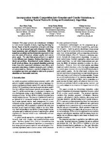
[Download] [PDF] Open-Channel Flow Download ... - WordPress.com

Open Channel Flow-Chaudhry - Professor Manouchehr Heidarpour

Open-Channel Flow Through Simulated Vegetation ... - Core

Flood plain contribution to open channel flow structure - Hydrologie.org

Mean flow and turbulence in vegetated open channel flow

Evolutionary Computation - Semantic Scholar

Evolutionary Computation: An Overview

Swarm and Evolutionary Computation

Swarm and Evolutionary Computation