remote sensing Article
Urbanization Effects on Vegetation and Surface Urban Heat Islands in China’s Yangtze River Basin Rui Yao 1 , Lunche Wang 1, *, Xuan Gui 1 , Yukun Zheng 1 , Haoming Zhang 1 and Xin Huang 2,3, * 1
2 3
*
Laboratory of Critical Zone Evolution, School of Earth Sciences, China University of Geosciences, Wuhan 430074, China;
[email protected] (R.Y.);
[email protected] (X.G.);
[email protected] (Y.Z.);
[email protected] (H.Z.) School of Remote Sensing and Information Engineering, Wuhan University, Wuhan 430079, China State Key Laboratory of Information Engineering in Surveying, Mapping and Remote Sensing, Wuhan University, Wuhan 430079, China Correspondence:
[email protected] (L.W.);
[email protected] (X.H.); Tel.: +86-133-4988-9828 (L.W.); +86-027-68778546 (X.H.)
Academic Editors: James Campbell and Prasad S. Thenkabail Received: 12 April 2017; Accepted: 29 May 2017; Published: 30 May 2017
Abstract: In the context of rapid urbanization, systematic research about temporal trends of urbanization effects (UEs) on urban environment is needed. In this study, MODIS (Moderate Resolution Imaging Spectroradiometer) land surface temperature (LST) data and enhanced vegetation index (EVI) data were used to analyze the temporal trends of UEs on vegetation and surface urban heat islands (SUHIs) at 10 big cities in Yangtze River Basin (YRB), China during 2001–2016. The urban and rural areas in each city were derived from MODIS land cover data and nighttime light data. It was found that the UEs on vegetation and SUHIs were increasingly significant in YRB, China. The ∆EVI (the UEs on vegetation, urban EVI minus rural EVI) decreased significantly (p < 0.05) in 9, 7 and 5 out of 10 cities for annual, summer and winter, respectively. The annual daytime and nighttime SUHI intensity (SUHII; urban LST minus rural LST) increased significantly (p < 0.05) in 10 and 4 out of 10 cities, respectively. The increasing rate of daytime SUHII and the decreasing rate of ∆EVI in old urban areas were much less than the whole urban area (0.034 ◦ C/year vs. 0.077 ◦ C/year for annual daytime SUHII; 0.00209/year vs. 0.00329/year for ∆EVI). The correlation analyses indicated that the annual and summer daytime SUHII were significantly negatively correlated with ∆EVI in most cities. The decreasing ∆EVI may also contribute to the increasing nighttime SUHII. In addition, the significant negative correlations (r < −0.5, p < 0.1) between inter-annual linear slope of ∆EVI and SUHII were observed, which suggested that the cities with higher decreasing rates of ∆EVI may show higher increasing rates of SUHII. Keywords: surface urban heat island; vegetation; urbanization; temporal trend; Yangtze River Basin
1. Introduction Urbanization, the process of the agricultural-based rural society transforming to the industrial-based urban society, is becoming an increasingly serious problem. The urban population around the world has doubled from 1750 million in 1980 to 3571 million in 2010, and this number will reach up to 5058 million in 2030 [1]. In addition, the increasing rate of global urban area is twice as fast as population growth [2]. Rapid urbanization can bring a series of problems, including urban heat island [3], reduction of cropland and vegetation coverage [4], changes of land surface phenology [5], and air pollution [6]. Thus, the magnitudes, the temporal trends and the relationships between the above-mentioned problems due to urbanization should be comprehensively investigated.
Remote Sens. 2017, 9, 540; doi:10.3390/rs9060540
www.mdpi.com/journal/remotesensing
Remote Sens. 2017, 9, 540
2 of 17
One of the serious problems due to urbanization is the reduction of vegetation coverage. Vegetation plays very important roles in terrestrial ecosystems and can bring a lot of benefits to human society [7]. The forest is even likened to the lungs of the earth. Vegetation can mitigate the air pollution [8], noise pollution [9] and urban heat island [10]; it can also prevent the loss of soil and water through retention of precipitation [11], and alleviate the greenhouse effect through absorbing CO2 [12]. However, a series of benefits from vegetation will also be lost due to urbanization; for example, urbanization can transform the forest and cropland to built-up land, reducing the vegetation coverage directly. Urban heat island (UHI), a problem due to urbanization, refers to the phenomenon where the air temperature in the city is higher than that of the countryside, which has a large amount of negative effects [3]. It can influence vegetation activity [5] and climate [13]. In addition, UHI can affect human health [14] and energy consumption [15,16]. The UHI may lead to more serious problems in the context of global warming [17]; for example, Goggins et al. [18] indicated when the air temperature increased 1 ◦ C (above 29 ◦ C), mortality can increase 4.1% accordingly. Remote sensing provided a new method for studying the earth surface process, including urbanization [19], hydrology [20], agriculture [21], UHI [3] and disaster monitoring [22]. The urbanization effects (UEs) on vegetation have been investigated in many studies; for example, Zhou et al. [7] used the MODIS enhanced vegetation index (EVI) data to study the UEs on vegetation. The results indicated that the EVI decreased significantly with increasing urban development intensity for most cities in China. Liu et al. [23] used normalized difference vegetation index (NDVI) to analyze the UEs on vegetation for 50 cities in the world during 1981–2010, which indicated that urbanization did not necessarily lead to decreasing vegetation (NDVI), but decreasing ∆NDVI between urban and rural areas was observed. The temperature monitored by remote sensing was land surface temperature (LST), which was different from the air temperature monitored by the weather stations. Therefore, the UHI monitored by remote sensing was surface UHI (SUHI). Peng et al. [10] used MODIS LST data to study the SUHI intensity (SUHII) at 419 global big cities during 2003–2008 and the average daytime and nighttime SUHII were 1.5 ◦ C and 1.1 ◦ C, respectively. Zhou et al. [3] studied the SUHII at 32 major Chinese cities and the SUHII varied greatly by season, location and background climates. Alves [24] indicated that the SUHII was 12 ◦ C in Ceres and Rialma (Brazil). However, few studies have been conducted focusing on the temporal trends of UEs on SUHII and its relationships with decreasing vegetation. Quan et al. [25] studied the relationships between temporal trends of nighttime LST and NDVI or climatic parameters in Beijing during 2000–2012 and the results showed that the temporal trend of urban nighttime LST was negatively correlated with NDVI, but an insignificant correlation was found in rural areas. Wang et al. [26] indicated that the SUHII increased significantly at outskirts of Phoenix (United States) in June during 2000–2014, which can primarily be attributed to the decreasing vegetation. Detailed study at the regional or global scale is still needed. China has undergone fast urbanization in past decades. The proportion of urban population to total population in China was 35.9% in 2000, 55.6% in 2015, and it is predicted that this data will reach up to 68.7% in 2030 [1]. The Yangtze River Basin (YRB) plays an important role in economic development, food production and water supply in China [27,28]. For the purpose of comprehensively understanding the UEs on environment, decision-making and human beings, it is essential to systematically study the temporal trends of UEs on urban environment. Therefore, we provided a comprehensive study of UEs on vegetation and SUHII and their potential relationships. The main purpose of this study were to: (1) reveal the 16-year averaged UEs on vegetation and SUHII in YRB, China during 2001–2016; (2) study the temporal trends of UEs on vegetation and SUHII for the whole study period; (3) examine the relationships between UEs on vegetation and SUHII. Our study can provide an important reference to study the temporal trends of UEs on the urban environment, which will be helpful for better understanding of the relationships between UEs on vegetation and SUHII.
Remote Remote Sens. Sens. 2017, 2017, 9, 9, 540 540
33 of of 17 17
2. Data and Methods 2. Data and Methods 2.1. Study Area 2.1. Study Area The YRB (total area: 1.8 million km2, population: 400 million) is located at the southern part of The YRB (total area: 1.8 million km2 , population: 400 million) is located at the southern China (Figure 1). The YRB is generally characterized by a subtropical monsoon climate. The annual part of China (Figure 1). The YRB is generally characterized by a subtropical monsoon climate. total precipitation in YRB is about 1070 mm, and the annual mean temperature is about 17 °C The annual total precipitation in YRB is about 1070 mm, and the annual mean temperature is about [29,30]. The Yangtze River Delta urban agglomeration (YRDUA) is one of the most famous urban 17 ◦ C [29,30]. The Yangtze River Delta urban agglomeration (YRDUA) is one of the most famous urban agglomerations in the world [31]. In this study, YRDUA (including Shanghai, Suzhou, Changzhou agglomerations in the world [31]. In this study, YRDUA (including Shanghai, Suzhou, Changzhou and Wuxi) and another nine municipalities or provincial capitals were chosen, including Chengdu and Wuxi) and another nine municipalities or provincial capitals were chosen, including Chengdu (CD), Guiyang (GY), Chongqing (CQ), Kunming (KM), Wuhan (WH), Nanchang (NC), Changsha (CD), Guiyang (GY), Chongqing (CQ), Kunming (KM), Wuhan (WH), Nanchang (NC), Changsha (CS), (CS), Hefei (HF) and Nanjing (NJ) (Figure 1). Hefei (HF) and Nanjing (NJ) (Figure 1).
Figure Figure 1. 1. The The spatial spatial distributions distributions of of the the 10 10 cities cities in in Yangtze YangtzeRiver River Basin, Basin, China, China, including including Chengdu Chengdu (CD), (GY), Chongqing (CQ), Wuhan (WH), Changsha (CS), Nanchang (NC), (CD),Kunming Kunming(KM), (KM),Guiyang Guiyang (GY), Chongqing (CQ), Wuhan (WH), Changsha (CS), Nanchang Hefei (NJ) and Yangtze River Delta (YRDUA). The index is (NC), (HF), HefeiNanjing (HF), Nanjing (NJ) and Yangtze RiverUrban Delta Agglomeration Urban Agglomeration (YRDUA). Themap index South China Sea, and the map projection system is Xi’an 1980. map is South China Sea, and the map projection system is Xi’an 1980.
2.2. 2.2. Land Cover Cover Data Data In version 4 stable nighttime light data annual composite, 30” spatial30″ resolution, In this thisstudy, study, version 4 stable nighttime light(SNLD; data (SNLD; annual composite, spatial digital number (DN) ranging from 0 to from 63) during and MODIS land cover (LCD; resolution, digital number (DN) ranging 0 to 63)2001–2013 during 2001–2013 and MODIS landdata cover data MCD12Q1; combined Terra and Aquaand satellite; composite; 500 m spatial (LCD; MCD12Q1; combined Terra Aqua annual satellite; annual composite; 500resolution m spatial(resampled resolution to 1000 m)) during 2001–2013 were combinedwere to generate the urban and rural (resampled to 1000 m)) during 2001–2013 combined to generate the areas urban[31,32]. and rural areas [31,32]. 2.3. MODIS LST and EVI Data
2.3. MODIS MODIS LST LST and dataEVI hasData been widely used to study the SUHIs at regional scale [3,10,31–36] because of its MODIS high accuracy, wide coverage and high temporal resolution (four passscale every[3,10,31–36] day; Terra LST data has been widely used to study the SUHIs attimes regional satellite: 10:30 a.m. and 10:30 p.m. local time, Aqua satellite: 1:30 a.m. and 1:30 p.m. local time). this because of its high accuracy, wide coverage and high temporal resolution (four times passIn every study, the LST was derived from MOD11A2 data (Terra satellite, 1 km resolution, day day; Terra satellite: 10:30 a.m. andthe 10:30 p.m. local time, Aqua satellite: 1:30spatial a.m. and 1:30 p.m.8local composite) for the period 2001–2016. The accuracy of MODIS LST product has been validated by time). In this study, the LST was derived from the MOD11A2 data (Terra satellite, 1 km spatial previous studies: the errors are within ± 1 K in 39 of 47 cases [37,38]. resolution, 8 day composite) for the period 2001–2016. The accuracy of MODIS LST product has
been validated by previous studies: the errors are within ±1 K in 39 of 47 cases [37,38].
Remote Sens. 2017, 9, 540
4 of 17
Several studies have showed that enhanced vegetation index (EVI) is more appropriate for monitoring vegetation dynamics in urban areas usually covered by sparse vegetation than the NDVI [39–41]. In this study, MODIS EVI data (MOD13A2, Terra satellite, 1 km spatial resolution, 16 day composite) from 2001 to 2016 was used to extract the vegetation information. In this study, the MODIS data was first reprojected and mosaicked using MODIS reprojection tool [42], and then averaged (ignoring no data value) into annual (12 months), summer (June to August) and winter (December to February) before it was processed further. 2.4. Extraction of Urban Area The SNLD cannot be used directly because of these problems: (a) lack of calibration; (b) sensor deterioration; and (c) differences of radiometric performance [43–45]. Therefore, a series of calibration methods were performed (intercalibration, intra-annual composition and inter-annual calibration) according to Liu et al. [45] to solve these problems. Taiwan province was used as a reference area and the F18 2010 was used as reference data to perform the intercalibration. Detailed information about these methods can be found in Liu et al. [45]. The intercalibration equations are as follows (Equation (1)): A = C1 × B2 + C2 × B + C3 (1) where B is the initial DN value of SNLD, A is the intercalibrated DN value, C1, C2, and C3 are the coefficients (Table 1). Table 1. The coefficients of calibration equations for intercalibrating the stable nighttime light (SNLD) data. Data
C1
C2
C3
R2
F142001 F142002 F142003 F152001 F152002 F152003 F152004 F152005 F152006 F152007 F162004 F162005 F162006 F162007 F162008 F162009 F182010 F182011 F182012 F182013
−0.0176 −0.0131 −0.0147 −0.0109 −0.0066 −0.0182 −0.0178 −0.0173 −0.0158 −0.0186 −0.0141 −0.021 −0.0133 −0.0098 −0.0105 −0.0121 0 −0.0037 −0.0013 −0.0006
2.0892 1.7978 1.888 1.6914 1.4128 2.1077 2.0849 2.0518 1.9692 2.1455 1.8747 2.2854 1.8456 1.6158 1.6601 1.7534 1 1.2136 1.0635 1.0114
−0.8501 0.302 0.7129 −1.3106 −0.5183 0.22 0.1465 0.397 0.066 0.235 −0.6434 −0.9842 −0.8746 −0.4421 −0.6306 0.4396 0 0.7621 0.5368 1.869
0.96 0.96 0.96 0.94 0.94 0.94 0.96 0.94 0.96 0.98 0.94 0.95 0.96 0.96 0.96 0.97 1.00 0.97 0.98 0.97
In this study, SNLD and MODIS LCD were used to generate the urban and rural areas. Both data have their advantages and disadvantages. We used the MODIS LCD to generate the urban areas in WH and there were no large variations of urban areas between 2001 and 2013 (Figure 2a,b and Figure 3a,b), which does not meet the actual characteristics of rapid urbanization in WH in past decades [46]. This suggested that the MODIS LCD is not suitable for studying the inter-annual urbanization. In addition, the SNLD was frequently used to generate the urban area across different years [44,45]. However, the SNLD data has a blooming effect; the urban area extracted from SNLD was usually larger than the real urban area [44,47]. Figures 2c and 3c showed that the urban areas at WH extracted from SNLD
Remote Sens. 2017, 9, 540 Remote Sens. 2017, 9, 540
5 of 17 5 of 17
contained the Yangtze River and some lakes, which should be removed in SUHI’s study [3,10,48]. was usually larger than the real urban area [44,47]. Figures 2c and 3c showed that the urban areas at In addition, MODIS LCD can extract thethe water bodyRiver accurately (Figures andshould 3d). Therefore, we first WH extracted from SNLD contained Yangtze and some lakes, 2d which be removed used in theSUHI’s SNLDstudy to generate the areas at each citycan in extract the year and 2013, DN > 50(Figures was used to [3,10,48]. Inurban addition, MODIS LCD the2001 water body accurately extract areas according to Liu al. [23]. Secondly, takeareas the union water 2d the andurban 3d). Therefore, we first used theetSNLD to generate thewe urban at eachof city in thebody year from 13 land cover maps using MODIS LCD during 2001–2013. Next, we excluded the union area 2001 and 2013, DN > 50 was used to extract the urban areas according to Liu et al. [23]. Secondly, of wewater the unionareas of water body from from the 13 land cover using LCD duringextract 2001–2013. Next, area bodytake from urban derived SNLD, somaps that we canMODIS more accurately the urban we 2e) excluded the union area temperature of water bodyzone from (Figure urban areas from the SNLD, area so that can for (Figure and cover the high 3e). derived The amount of urban in we 10 cities more accurately extract the urban area (Figure 2e) and cover the high temperature zone (Figure 3e). the year 2001 and 2013 can be found in Table 2. We further compared the urban area extracted using The amount of urban area in 10 cities for the year 2001 and 2013 can be found in Table 2. We further nighttime data with that from Landsat data (maximum likelihood classification method). The results compared the urban area extracted using nighttime data with that from Landsat data (maximum showed that the urban area extracted using the method in this study was larger than that from Landsat likelihood classification method). The results showed that the urban area extracted using the data method (Table 2); is appropriate for this duedata to these (a) the of SUHI in however, this studyitwas larger than that fromstudy Landsat (Tablereasons: 2); however, it isfootprint appropriate was larger than the actual urban size according to previous studies [40,48,49]; (b) the urbanization for this study due to these reasons: (a) the footprint of SUHI was larger than the actual urban size primarily occurred in the suburban areas according to previousprimarily studies [26,36]; (c)inthe period in according to previous studies [40,48,49]; (b) the urbanization occurred thestudy suburban this study was 2001–2016, the land cover maps(c)used were during 2001–2013, urban area areas according to previous studies [26,36]; the study period in this studyand wasthe 2001–2016, the may land cover 2014–2016. maps used were during 2001–2013, the andbuffer the urban may expand expand during Finally, we generated zonearea between 20 andduring 25 km 2014–2016. from the urban weexcluded generatedthe thepixel bufferwith zoneDN between 20 and 25in km from the km urban areas,and anddefined we excluded areas,Finally, and we > 10 (SNLD) the 20–25 buffer it as rural the pixel with DN > 10 (SNLD) in the 20–25 km buffer and defined it as rural area [5,41]. The rural area [5,41]. The rural areas in this study were set larger than previous studies, since the footprint of areas in this study were set larger than previous studies, since the footprint of UEs was much larger UEs was much larger than the urban areas in previous studies [5,40,48,49]. We did not select larger than the urban areas in previous studies [5,40,48,49]. We did not select larger buffer zones for buffer zones for reducing the uncertainties due to different climate conditions and topography [48]. reducing the uncertainties due to different climate conditions and topography [48]. The accuracy of The accuracy of this methodurban of defining urban area may lower than using theresolution higher spatial this method of defining area may be lower thanbe those using thethose higher spatial resolution (e.g., Landsat data), is fast and enough for matching thespatial 1 km resolution spatial resolution imagesimages (e.g., Landsat data), but it isbut fastit and enough for matching the 1 km of of MODIS LST (MOD11A2) (MOD11A2)data. data. Thus, method be applied at national, MODISEVI EVI(MOD13A2) (MOD13A2) and LST Thus, thisthis method can can be applied at national, continental global scale future. continental andand global scale in in future.
Figure 2. The comparison of different data and methods of extracting the urban areas or water body
Figure 2. The comparison of different data and methods of extracting the urban areas or water body in WH: (a) urban areas in WH extracted from MODIS land cover data (LCD) in 2001; (b) urban areas in WH: (a) urban areas in WH extracted from MODIS land cover data (LCD) in 2001; (b) urban areas in WH extracted from MODIS LCD in 2013; (c) urban areas in WH extracted from stable nighttime in WH extracted from MODIS LCD in 2013; (c) urban areas in WH extracted from stable nighttime light data in 2013; (d) the union areas of water body in WH extracted from MODIS LCD; (e) SNLD light and dataMODIS in 2013;LCD (d) the union areas to of water body WHareas extracted from MODIS LCD; map (e) SNLD were combined produce the in urban in WH. The background was and MODIS LCDOLI were combined produce Landsat image from 16 to August 2013.the urban areas in WH. The background map was Landsat OLI image from 16 August 2013.
Remote Sens. 2017, 9, 540 Remote Sens. 2017, 9, 540
6 of 17 6 of 17
Figure 3. The Figure 3. The comparison comparison of of different different data data and and methods methods of of extracting extracting the the urban urban areas areas or or water water body body in WH: (a) urban areas in WH extracted from MODIS LCD in 2001; (b) urban areas in WH extracted in WH: (a) urban areas in WH extracted from MODIS LCD in 2001; (b) urban areas in WH extracted from from MODIS MODIS LCD LCD in in 2013; 2013; (c) (c) urban urban areas areas in in WH WH extracted extracted from from stable stable nighttime nighttime light light data data in in 2013; 2013; (d) the union unionareas areasofofwater waterbody body WH extracted from MODIS LCD; (e) SNLD and MODIS (d) the in in WH extracted from MODIS LCD; (e) SNLD and MODIS LCD LCD were were combined to produce theareas urban areasThe in WH. The background map was the land surface combined to produce the urban in WH. background map was the land surface temperature temperature (LST, in WH2013. in summer, 2013. (LST, ◦ C) in WH in°C) summer, Table 2. The The amount amount of of urban urban area area in in the the 10 10 cities cities for Table 2. for the the year year 2001 2001 and and 2013. 2013. Unit: Unit: square squarekilometer. kilometer. The numbers in in parentheses parentheses indicate indicate the the area area extracted extracted from from Landsat Landsat data. data. The numbers
YRDUA NJ HF WH CS YRDUA NJ HF WH CS 3376 489 193 453 191 20014313 3376 646 489 259 193 499453 191 216 2002 4313 646 259 499 216 312 20035813 5813 842 842 311 311 579579 312 390 20046767 6767 948 948 344 344 667667 390 20057831 7831 1003 1003378 378 748748 405 405 20068389 8389 1013 1013413 413 763763 441 441 2007 8919 1077 516 863 521 8919 1077 516 863 521 2008 9788 1128 594 893 537 537 20099788 9840 1128 1130594 602 893893 538 538 20109840 10,8471130 1261602 690 893932 557 2011 11,873 1359 763 1031 568 10,847 1261 690 932 557 2012 11,945 1360 764 1031 575 11,873 1359 763 1031 568 1443 844 1339 790 2013 11,94513,0731360 (1335)764 (584) 1031 (1088) 575 (554) 1443 844 1339 790 2013 13,073 (1335) (584) (1088) (554) 2.5. Calculation of UEs on Vegetation and SUHII 2001 2002 2003 2004 2005 2006 2007 2008 2009 2010 2011 2012
NC CQ CQ 118 277 118 277 169 296 169 296 292 292 381381 331 331 438438 334 489489 334 341 547547 341 393 566 393 566 418 568 418 418 585568 418 429 587585 448 587587 429 448 614 448 587 533 808 448 614 (410) (716) 533 808 (410) (716) NC
CD KM GY KM GY 387 298 85 387 423 298 30885 92 423 308 92 598 598 329 329249 249 677 677 352 352255 255 711 711 392 392259 259 867 867 423 423259 259 909 463 259 909 463 259 934 492 259 1100 934 596 492275 259 12481100 616 596281 275 12581248 627 616299 281 1258 1258 680 627299 299 1591 727 385 (1317)1258(571) 680 (295) 299 1591 727 385 (1317) (571) (295) CD
The SUHIIofwas using 2.5. Calculation UEscalculated on Vegetation andEquation SUHII (2) according to previous studies [3,10]:
The SUHII was calculated using according to previous studies [3,10]: ∆LSTEquation (SUHII) =(2) LST − LST urban
rural
∆LST (SUHII) = LSTurban − LSTrural
(2)
(2)
Remote Sens. 2017, 9, 540
7 of 17
where the LSTurban and LSTrural were the LST in urban and rural areas, respectively, and the ∆LST represented the SUHII. The urban and rural areas were derived from the land cover maps in the year 2013. The UEs on vegetation were calculated as (Equation (3)): ∆EVI = EVIurban − EVIrural
(3)
where the EVIurban and EVIrural were the EVI in urban and rural, respectively, the ∆EVI represented the UEs on vegetation. In this study, we calculated the SUHII and ∆EVI during 2001–2016 using the static land cover map in the year 2013. The purpose was to compare the SUHII or ∆EVI in the same places across different years [5]. In addition, the urban area in the year 2001 was defined as old urban area (OUA), and the urbanized area (UA) was defined as the differences between the urban area in the year 2001 and 2013. Annual, summer (from June to August) and winter (from December to February) averaged SUHII and ∆EVI in each year were calculated separately. Linear regression analyses were performed in SPSS 22.0 to examine the temporal trends of UEs on vegetation (∆EVI) and SUHII in each city. The relationships between SUHII and ∆EVI were analyzed using Pearson’s correlation analysis. 3. Results 3.1. 16-Year Averaged UEs on Vegetation and SUHII Table 3 showed the 16-year averaged UEs on vegetation in each city; all cities showed negative UEs on vegetation (∆EVI < 0), ranging from −0.157 at CQ in summer to −0.042 at YRDUA in winter. The UEs on vegetation (i.e., ∆EVI) differed greatly in each season. The variations of ∆EVI were more obvious in summer (−0.119 averaged for 10 cities), followed by annual (−0.088 averaged for 10 cities) and winter (−0.060 averaged for 10 cities). Table 3. 16-year averaged urbanization effects (UEs) on vegetation (∆EVI) at 10 cities in Yangtze River Basin (YRB), China. The average data in the table is the mean value of 10 cities. City
Annual
Summer
Winter
CD CS CQ GY HF KM NC NJ WH YRDUA Average
−0.074 −0.106 −0.101 −0.082 −0.082 −0.115 −0.088 −0.069 −0.093 −0.071 −0.088
−0.092 −0.153 −0.157 −0.115 −0.100 −0.126 −0.122 −0.099 −0.137 −0.087 −0.119
−0.060 −0.072 −0.069 −0.044 −0.055 −0.105 −0.051 −0.043 −0.064 −0.042 −0.060
The 16-year averaged SUHII in each city was shown in Table 4; nearly all cities showed positive SUHII (except certain cities in winter). The seasonal variations of daytime SUHII were similar to those for ∆EVI. The highest SUHII was observed on a summer day (3.07 ◦ C averaged for 10 cities), ranging from 2.43 ◦ C at WH to 4.49 ◦ C at KM. In contrary, the lowest SUHII was found on a winter day (0.41 ◦ C averaged for 10 cities), ranging from −0.46 ◦ C at WH to 1.38 ◦ C at KM. However, nighttime SUHII was relatively stable across seasons (0.88 ◦ C, 1.09 ◦ C and 0.70 ◦ C averaged for 10 cities for annual, summer and winter, respectively), ranging from −0.07 ◦ C at HF in winter to 2.36 ◦ C at KM in summer.
Remote Sens. 2017, 9, 540 Remote Sens. 2017, 9, 540
8 of 17 8 of 17
Table 4. 16-year averaged surface urban heat island intensity (SUHII) at 10 cities in YRB, China.
Annual Annual Summer Summer Winter Table 4. 16-year averaged surface urban heat island intensity (SUHII) at 10Winter cities in YRB, China.
City
CD City CS CD CQ CS GY CQ HF GY KM HF KM NC NC NJ NJ WH WH YRDUA YRDUA Average Average
Day (°C) Annual 2.26 Day (◦ C)
1.47
2.26 1.70 1.47 1.96 1.70 1.43 1.96 2.69 1.43 2.69 1.18 1.18 1.15 1.15 0.71 0.71 1.75 1.75 1.63 1.63
Night (°C) Annual 0.71 Night (◦ C)
0.56
0.71 0.81 0.56 1.26 0.81 0.29 1.26 1.83 0.29 1.83 0.72 0.72 0.76 0.76 0.84 0.84 1.02 1.02 0.88 0.88
Day (°C) Summer 3.00 Day (◦ C)
3.29
3.00 3.02 3.29 2.79 3.02 2.79 2.79 4.49 2.79 4.49 3.37 3.37 2.77 2.77 2.43 2.43 2.74 2.74 3.07 3.07
Night (°C) Summer 1.28 Night (◦ C) 1.12 1.28 1.51 1.12 1.57 1.51 0.45 1.57 2.36 0.45 2.36 0.82 0.82 0.30 0.30 0.76 0.76 0.70 0.70 1.09 1.09
Day (°C) Winter 1.13 Day (◦ C)
−0.16
1.13 0.46 −0.16 1.04 0.46 0.08 1.04 1.38 0.08 1.38 −0.33 −0.33 0.06 0.06 −0.46 −0.46 0.87 0.87 0.41 0.41
Night (°C) Winter 0.80 Night (◦ C) 0.08 0.80 0.27 0.08 0.60 0.27 −0.07 0.60 1.25 −0.07 1.25 0.88 0.88 0.95 0.95 0.84 0.84 1.39 1.39 0.70 0.70
3.2. Trends of of ∆EVI ∆EVI in in YRB YRB during during 2001–2016 2001–2016 3.2. Temporal Temporal Trends Figure showed the Figure 44 showed the temporal temporal trends trends of of ∆EVI ∆EVI in in YRB YRB averaged averaged for for 10 10 cities cities during during 2001–2016; 2001–2016; the annual, summer and winter ∆EVI decreased significantly at the rate of −0.00329/year the annual, summer and winter ∆EVI decreased significantly at the rate of −0.00329/year (p (p 0.05) at NJ. The significant decreasing trends of ∆EVI were also observed in halfofofthethe cities (5 of out in ranging winter, from ranging from −0.00607/year (p CD < 0.01) at CD to in half cities (5 out 10)of in 10) winter, −0.00607/year (p < 0.01) at to 0.00009/year 0.00009/year (p >Table 0.05) 6atshowed NJ. Table showed the temporal trends of ∆EVIalthough in OUAs;the although the (p > 0.05) at NJ. the6 temporal trends of ∆EVI in OUAs; significant significant decreasing trends of ∆EVI were observed in 9 out of 10 cities, the decreasing rates of decreasing trends of ∆EVI were observed in 9 out of 10 cities, the decreasing rates of ∆EVI in OUAs ∆EVI in OUAs were much less than the whole urban areas (−0.00209/year vs. −0.00329/year were much less than the whole urban areas (−0.00209/year vs. −0.00329/year averaged for 10 cities). averaged for 10 cities). The city showed an insignificant decreasing of ∆EVI at NJ, the and EVI The city showed an insignificant decreasing trend of ∆EVI at NJ,trend and the EVI in bothand OUA in both OUA and rural areas showed insignificant increasing trends (0.00039/year and 0.00056/year rural areas showed insignificant increasing trends (0.00039/year and 0.00056/year for OUA and rural for OUA and rural areas, respectively). areas, respectively).
∆EVI averaged for 10 cities during 2001–2016. Figure 4. The temporal trends of ∆EVI
Remote Sens. 2017, 9, 540
9 of 17
Remote Sens. 2017, 9, 540
9 of 17
Table at 10 10 cities citiesin inYRB, YRB,China. China. Table5.5.Temporal Temporaltrends trendsof of ∆EVI ∆EVI at City City CD CD CS CS CQ CQ GY GY HF HF KM KM NC NC NJ NJ WH WH YRD Average YRD Average
Annual Annual (/Year) (/Year) Summer Summer (/Year) (/Year) −0.00538 ** −0.00563 −0.00538 ** −0.00563** ** −0.00460 −0.00630 −0.00460 ** ** −0.00630** ** −0.00529 −0.00614 −0.00529 ** ** −0.00614** ** −0.00336 ** ** −0.00508** ** −0.00336 −0.00508 −0.00392 ** ** −0.00572** ** −0.00392 −0.00572 − 0.00308 ** − 0.00247 −0.00308 ** −0.00247 −0.00216 −0.00487 ** −0.00216 −0.00487 −0.00110 ** −0.00044** −0.00110 −0.00189 ** ** −−0.00044 0.00376 ** −0.00189 −0.00376 −0.00211 ** ** −0.00113** −0.00329 ** ** −−0.00113 0.00415 ** −0.00211 −0.00329 ** −0.00415 ** Significance levels: ** p < 0.01.
Winter (/Year) Winter (/Year) −0.00607 ** ** −0.00607 −0.00310 ** −0.00310 ** −0.00390 ** ** −0.00390 −0.00171 −0.00171 ** ** −0.00220 −0.00220 −0.00257 −0.00257 ** ** −0.00083 −0.00083 0.00009 0.00009 −0.00084 −0.00084 −0.00051 −0.00217 ** −0.00051 −0.00217 **
Significance levels: ** p < 0.01. Table 6. Temporal trends of ∆EVI and SUHII in old urban areas (OUAs) in the YRB, China. Table 6. Temporal trends of ∆EVI and SUHII in old urban areas (OUAs) in the YRB, China. City CD CS CQ GY HF KM NC NJ WH YRD Average
Annual Daytime SUHII
Annual Nighttime SUHII
Annual ∆EVI
CityDaytime SUHII Annual (°C/Year) Annual Nighttime SUHII (°C/Year) (/Year) Annual ∆EVI (/Year) (◦ C/Year) (◦ C/Year) 0.020 0.020 −0.00285 ** CD 0.020 0.020 −0.00285 ** 0.045 ** 0.052 ** −0.00303 ** CS 0.045 ** 0.052 ** −0.00303 ** 0.082 ** 0.082 ** 0.053**** ** CQ 0.053 −0.00388−0.00388 ** 0.027 0.006 ** GY 0.027 0.006 −0.00229−0.00229 ** HF 0.014 0.065 −0.00276−0.00276 ** 0.014 0.065**** ** KM 0.029 0.024 −0.00148*−0.00148* 0.029 0.024**** NC 0.029 * −0.003 −0.00154 ** 0.029 * −0.003 −0.00154 ** NJ 0.031 * 0.025 −0.00017 0.031 * 0.025 WH 0.033 0.012 −0.00126 *−0.00017 0.033 0.012 * YRD 0.033 0.014 −0.00160−0.00126 * 0.033 0.034 ** 0.014 * Average 0.027 ** −0.00209 −0.00160 ** 0.034 ** Significance levels: * p < 0.05, 0.027 −0.00209 ** ** p < ** 0.01.
Significance levels: * p < 0.05, ** p < 0.01.
3.3.3.3. Temporal Trends of of SUHII Temporal Trends SUHIIininYRB YRBduring during2001–2016 2001–2016 Figure 5 showed averagedfor for10 10cities citiesduring during 2001–2016; Figure 5 showedthe thetemporal temporaltrends trendsof of daytime daytime SUHII SUHII averaged 2001–2016; thethe annual, summer and winter SUHII increased significantly for the whole study period. For daytime annual, summer and winter SUHII increased significantly for the whole study period. For ◦ C/year, p < 0.01), followed by annual SUHII SUHII, the highest increasing rate was in summer (0.144 daytime SUHII, the highest increasing rate was in summer (0.144 °C/year, p < 0.01), followed by ◦ C/year, p < 0.01) and winter SUHII (0.029 ◦ C/year, p < 0.01). Meanwhile, the increasing rates (0.077 annual SUHII (0.077 °C/year, p < 0.01) and winter SUHII (0.029 °C/year, p < 0.01). Meanwhile, the of increasing nighttime SUHII similarSUHII acrosswere different seasons 6);seasons the annual, summer winter rates ofwere nighttime similar across(Figure different (Figure 6); theand annual, ◦ ◦ nighttime increased significantly at the ratesignificantly of 0.023 C/year < 0.01), 0.033 C/year < 0.01) summerSUHII and winter nighttime SUHII increased at the(prate of 0.023 °C/year (p