Application of Finite Volume Integral Approach to Computing of 3D ...

Proceedings of EPAC 2004, Lucerne, Switzerland

APPLICATION OF FINITE VOLUME INTEGRAL APPROACH TO COMPUTING OF 3D MAGNETIC FIELDS CREATED BY DISTRIBUTED IRON-DOMINATED ELECTROMAGNET STRUCTURES O. Chubar, C. Benabderrahmane, O. Marcouille, F. Marteau, SOLEIL, France J. Chavanne, P. Elleaume, ESRF, France Abstract Iron-dominated electromagnet structures are traditionally considered as domain of applications of the finite element method (FEM). FEM computer codes provide high accuracy for "close circuit" type geometries, however they can be much less efficient for distributed geometries consisting of many spatially separated magnets interacting with each other. Examples of such geometries related to particle accelerators are insertion devices. Application of the finite volume integral approach implemented in the Radia 3D magnetostatics code to solving such geometries is described. In this approach, space around individual magnets does not require any meshing. An adaptive segmentation of iron parts, with the segmenting planes being roughly perpendicular or parallel to the expected directions of magnetic flux lines, minimizes dramatically the necessary CPU and memory resources. If geometry is, nevertheless, too big for its complete interaction matrix to fit into memory, a special scheme of relaxation "by parts" can be applied. The results of calculations made for two different types of electromagnet undulators for Synchrotron SOLEIL are presented.

INTRODUCTION The majority of 3D magnetostatics computer codes use currently the finite element method [1], [2]. This powerful and universal method has experienced considerable progress over the last two decades, and continues to attract now maximum of attention of software developers and users. In this article, we show that another approach, which is based on finite volume integrals, can be very efficient in solving 3D magnetostatics problems with distributed iron-dominated electromagnet structures, and can successfully complement the FEM. The approach to numerical solution of 3D boundary problems of magnetostatics, based on integral equations written with respect to finite volumes with magnetization, was suggested in 1970's, and implemented for the first time in the computer code GFUN [3], probably before any reliable 3D implementations of the FEM. Strong and weak points of the volume integral method, compared to the FEM, were discussed in [4] - [6]. The finite volume integral approach is used in the Radia 3D magnetostatics computer code [6], [7]. The original purpose of this code was CPU-efficient computation of the magnetic field and field integrals from permanent-magnet and hybrid type insertion devices for synchrotron radiation sources [8], [9]. The code appears to be also efficient for calculation of electromagnets for

particle accelerators [10], and allows for their 3D optimisation (e.g. quadrupole or dipole chamfers) [11]. In the following sections, the method basics are recalled, and applications for solving distributed iron-dominated structures of electromagnet undulators are described.

METHOD BASICS In the finite volume integral method, magnetostatics problem is solved by a relaxation procedure, which operates with an interaction matrix describing magnetic interaction between small volumes, and material relations. At calculation of the interaction matrix components and the field after the relaxation, analytical formulas are used. The use of the analytical formulas for the magnetic field allows to avoid any segmentation of free space between magnetized volumes (which is required in FEM), and minimizes the necessary segmentation density for iron parts of geometries. Thanks to these features, the volume integral method can be very fast.

Field from Uniformly Magnetized Volumes The magnetic field strength H(r) produced by N objects of arbitrary shape with their volumes uniformly magnetized according to vectors Mi, i = 1,2,..., N , at point with radius-vector r, can be expressed as N

H(r) = ∑ Q i (r) M i ,

(1)

i =1

where Qi(r), are 3 x 3 matrices, which depend on objects' geometries and r. Their components can be expressed via integrals over surfaces Si bounding the objects: Q i (r) =

1 2π

∫∫ Si

(r − ρ) ⊗ n S dS , | r − ρ |3

(2)

where ρ is radius-vector of a point on surface Si (which is varying at the integration), ns is unit vector normal to the surface Si at point ρ and directed outside the volume; the symbol ⊗ means dyadic (or tensor) product of 3D vectors, i.e., for any three vectors a, b, c: (a ⊗ b )c ≡ a(bc) . The surface integrals in Eq. (2) can be done analytically for various shapes, including an arbitrary polyhedron [7]. Other important magnetic characteristics, e.g. infinite magnetic field integrals along a straight line, can also be calculated analytically [6], [7]. Radia supports four basic space transformations: plane symmetry, rotation around an arbitrary axis, translation, and field inversion. Several space transformations can be combined into a new space transformation. The field created by an object, to which a space transformation was applied, is computed first in the object's local frame, and then transformed back to the laboratory frame.

1675

Proceedings of EPAC 2004, Lucerne, Switzerland

Interaction Matrix and Relaxation

EXAMPLES OF COMPUTATION

Let Hi be the magnetic field strength in the center of i-th object. This field can be calculated by the analogy with Eq. (1): N

H i = ∑ Q ik M k + H ex i , i = 1,2,..., N ,

(3)

k =1

where Hex i is external field in the center of i-th object. For each i and k, Qik is a 3 x 3 matrix, which is calculated by analytical formulas derived from Eq. (2). If a space transformation with some multiplicity m was applied to the k-th source object, then Qik is the sum of m contributions deduced after series of transformations of the observation point and field. For each of the N objects, the magnetization Mi is linked to the field strength Hi by a material relation: (4) M i = f i ( H i ), i = 1,2,..., N . The two common types of magnetic materials are: • linear anisotropic materials (e.g. permanent magnets), when f i (H i ) = χ i H i + M r i , where χ i is susceptibility tensor and Mr i is remanent magnetization for the material of i-th object, and • non-linear isotropic materials (e.g. iron), when fi (Hi ) = fi (| Hi |) Hi | Hi | , where f i (| Hi |) is a scalar function of magnetic field strength magnitude. The problem defined by Eqs. (3), (4) can be solved by an iterative relaxation procedure, which must be properly selected to ensure stable convergence [6]. For fast solution, the components of the interaction matrix Qik in Eq. (3) should be calculated before, and kept in memory during the relaxation. However, in those cases when this is not possible, the relaxation can be performed "by parts", i.e. all geometry can be split into several parts (preferably weakly interacting with each other), for which partial interaction matrices are calculated and stored in memory. Every part is repeatedly relaxed, with all other parts treated as external field sources. The magnetizations in all volumes are regularly updated; the calculation stops when they reach a required level of stability.

SOLEIL Undulator HU256 The 256-mm period undulator HU256 is designed to produce high flux of radiation in the VUV spectral range (from ~10 eV to ~300 eV) at Synchrotron SOLEIL [12]. Its conceptual design was done by SOLEIL, and the final optimisation by Budker Institute of Nuclear Physics (Novosibirsk). The structure is composed of a sequence of dipole yokes which produce vertical (Fig. 1-a) and horizontal (Fig. 1-b) magnetic fields. The vertical gap is 16 mm, the horizontal gap is 56 mm. The vertical dipole has 2 sets of coils: the main coil (closer to the centre in Fig. 1-a), and the modulation coil dedicated for quasiperiodic operation. Because of large horizontal gap, the shapes of the poles and coils of the horizontal dipoles (Fig. 1-b) had to be optimised to produce higher field at given maximal current of 250 A (24 coil turns). Even without solving the structure, one can guess that in the final assembly (Fig. 1-c), magnetic flux circulates essentially in the individual dipoles, with little interaction between them. Therefore initially, the vertical and horizontal dipoles were solved independently, with any influence of neighbouring dipoles being neglected. To ensure computation efficiency, the yoke models were segmented according to the rule described in the previous section. The segmentation is shown by thin lines on the surfaces of the yokes in Fig. 1-a, b. With this segmentation, solving of each of the dipoles for the accuracy of ~1% with respect to the peak field takes several minutes (at 2.4 GHz CPU clock). The results for the horizontal field are shown in Fig. 2 (dotted line). Solving the 3D problem for the total geometry with several periods of the central part, terminating poles (21 iron yokes in total), and upper and lower horizontal iron plates (Fig. 1-c), took more CPU time (several hours). Since the interaction matrix for the total geometry did not fit into computer memory, the scheme of relaxation "by parts" had to be applied. a) b)

Efficient Segmentation In the volume integral method, the density of segmentation required for a given accuracy of magnetic field outside the magnetized volumes is typically much smaller than in FEM. Nevertheless, the necessary density of segmentation (and so the memory and CPU resources) strongly depend on type of the segmentation. For the segmentation in the volume integral method to be efficient, it should produce 3D objects with faces which are roughly either perpendicular or parallel to the final directions of magnetization vectors (or magnetic flux lines). Even though the exact directions of the flux lines in iron are not known a priori, in most cases the general tendencies can be guessed before the solution. Besides, one can check the tendencies for magnetization directions by "pre-solving" the problem with preliminary uniform segmentation.

c)

Figure 1: Radia model of the undulator HU256, including the dipoles creating vertical (a) and horizontal (b) magnetic fields; and an assembly (c) with 3 complete periods, extremities (coil distribution according to "1/43/4" rule), and screening horizontal iron plates.

1676

Proceedings of EPAC 2004, Lucerne, Switzerland

Figure 2: Calculated magnetic field on the axis of the HU256 at maximal currents in the vertical and horizontal dipole coils (180 A, 16 turns and 250 A, 24 turns respectively). The on-axis horizontal and vertical magnetic fields calculated after solving the total geometry are shown in Fig. 2 by solid lines. One can see that the horizontal field obtained by solving the whole structure differs from the field calculated without taking into account magnetic interaction between the yokes, essentially at the locations of the vertical dipoles. This can be explained by partial "screening" of the field by the vertical dipole yokes, which have a small vertical gap. This effect influences the low-energy spectral cut-off value of the verticallypolarised emission from this undulator.

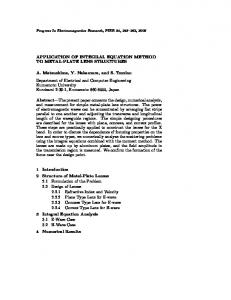
ESRF Undulator EMPHU (SOLEIL version) The electromagnet/permanent-magnet helical undulator (EMPHU), which has been designed at ESRF [13], represents another type of distributed iron-dominated structure. In this structure, the vertical magnetic field is created by continuous upper and lower yokes with many poles (see Fig. 3), and a wiggling coil. The structure allows for switching of the vertical field with the repetition rate up to 10 Hz. The horizontal magnetic field is created by permanent magnets (Sm2Co17). In the ESRF version, the undulator period is 80 mm; SOLEIL considers reducing the period down to 65 mm. The calculated vertical and horizontal magnetic fields are shown in Fig. 4. With the segmentation shown in Fig. 3, Radia calculates the field on the undulator axis with the estimated accuracy 1-3% (with respect to the peak field), which is sufficient for various optimisations of the structure. Since the interaction matrix of the whole geometry fits into memory, the calculation time is only several minutes.

CONCLUSION The finite volume integral approach can be efficiently applied for solving 3D problems of magnetostatics with distributed iron-dominated electromagnet structures. Numerical solution can be obtained even in the case when interaction matrix of the whole geometry does not fit into computer memory. Because of high CPU-efficiency and flexibility, this approach is well suited for 3D optimisation of electromagnet and hybrid magnet structures.

Figure 3: Radia model of the EMPHU considered for SOLEIL.

Figure 4: Calculated on-axis magnetic field from the EMPHU at minimal vertical gap (16 mm) and maximal current in the coil (~280 A).

REFERENCES [1] OPERA-3D, Copyright Vector Fields Ltd, http://www.vectorfields.com. [2] FLUX3D, Copyright MagSoft Corporation, http://www.flux3d.com. [3] C.W.Trowbridge, "Application of Integral Equation Methods to the Numerical Solution of Magnetostatic and EddyCurrent Problems", in "Finite Elements in Electrical and Magnetics Field Problems", John Wiley, edited by M.V.K. Chari and P.P.Silvester, 1980, chapter 10, p.191. [4] C.W.Trowbridge, "Integral Equations Revisited", ICS Newsletter, February 1996. [5] L.Kettunen, K.Forsman, D.Levine, W.Gropp, "Volume integral equations in nonlinear 3-d magnetostatics". Internat. Journal of Numerical Methods in Engineering, 1995, vol.38, p.2655. [6] P.Elleaume, O.Chubar and J.Chavanne, "Computing 3D Magnetic Fields from Insertion Devices", PAC'97, p.3509. [7] O.Chubar, P.Elleaume and J.Chavanne, "A 3D Magnetostatics Computer Code for Insertion Devices", Journal of Synchrotron Radiation, 1998, vol.5, p.481. [8] J.Chavanne, P.Elleaume, P.VanVaerenbergh, "End field structures for linear/helical insertion devices", PAC'99, p.2665. [9] J.Bahrdt, W.Frentrup, A.Gaupp, M.Scheer, U.Englisch, "Magnetic field optimisation of permanent magnet undulators for arbitrary polarization", Nucl. Instrum. Meth., 2004, vol.A516, p.575. [10] A.Andersson, L-J.Lindgren and O.Chubar, "3D Calculations for the MAX-II Lattice Magnets", EPAC'98, p.1207. [11] Radia computation examples are available at: http://www.esrf.fr/machine/groups/insertion_devices/Codes/Radia/Radia.html

[12] O.Marcouille et.al., "New design of polarized electromagnetic undulators at SOLEIL", proceedings of SRI2003, AIP, p.207. [13] J.Chavanne, P..Elleaume, P.VanVaerenbergh, "A novel fast switching linear/helical undulator", EPAC'98, p.317.

1677