R.W. Ferrero. J. F. Rivera. Instituto de Energia Electrica. Universidad Nacional de San Juan. Argentina. Abstract-- We present a game theoretical approach to the.
184
IEEE Transactions on Power Systems, Vol. 13, No. 1, February 1998
APPLICATION OF GAMES WITH INCOMPLETE INFORMATION FOR PRICING ELECTRICITY IN DEREGULATED POWER POOLS S.M. Shahidehpour R.W. Ferrero J. F. Rivera Department of Electrical and Computer Engineering Instituto de Energia Electrica Illinois Institute of Technology Universidad Nacional de San Juan Chicago, IL 60616 Argentina ................................................................................ Abstract-- We present a game theoretical approach to the PoolCo problem of pricing electricity in deregulated energy Spot price Deryand marketplaces. We assume that an Independent System Generation Operator receives bids by Pool participants and defines transactions among participants by looking for the minimum price that satisfies the demand in the Pool. The competition among Pool participants is modeled as a non-cooperative game with incomplete information. We assume that each Pool participant knows its own operation costs but does not know his opponents’ operation costs. The game with incomplete information is transformed into a game with complete, but ............................................................................. imperfect, information and solved using the Nash equilibrium Figure 1: The PoolCo idea. The approach presented in this paper is geared towards providing support for pricing electricity in deregulated Pools. In Figure 1, bids by generators as well as loads create a spot Keywords-Power Systems Operation, Deregulated Power market for electricity. The spot price is set by the last generator dispatched by the I S 0 to balance PoolCo’s Pools, Spot Market, Game Theory generation and demand. We consider a loseless case in which the spot price [6] is the same in all buses and is referred to as I. INTRODUCTION Traditional resource scheduling methodologies [ 1-31 are p. The spot price “clears” the market. Transaction payments aimed to schedule generation resources in order to minimize by each participant are defined as the product of the spot price operation costs while supplying system loads. Generation and power transaction. Other pricing schemes [ 5 ]would result resources are controlled centrally and information regarding in different allocation of benefits among participants; cost and operational constraints is shared among participants. however, our approach is general enough to be used in other In this traditional approach, benefit maximization is obtained scenarios as well. trough cost minimization. The objective is to maximize each participant’s benefits The electric power industry is shifting from a scenario in regardless of PoolCo’s benefits; hence, earnings fkom which operation schedule in filly regulated to a new transactions should be maximized. In this regard, price competitive deregulated scenario, in which cost minimization definition by participant plays a very important role. The is not equivalent to benefit maximization [4]. In deregulated lower the market price, the higher the net power interchanged. power systems, emphasis is given to benefit maximization A seller has to evaluate the possibility of either selling more from the perspective of participants (namely, vertically power at a low per unit price or selling less at a high price per integrated utilities, independent power producer firms, unit of power. A similar analysis can be made for a buyer. cogenerators, distribution companies, etc.) rather than Each participant anticipates a bid that results in the highest maximization of system-wide benefits. benefits when transactions are defined by the ISO. Moreover, As deregulation evolves, pricing electricity becomes a major each participant defines bids based on incomplete information issue in the electric industry. Participants of deregulated on other participant’s bids. energy marketplaces are able to improve their benefits In [ 101 game theory was used by the IS0 to identify coalitions substantially by adequately pricing the electricity. The among participants. In this paper we present a game international experience and most of the existing proposals in theoretical [7-91 approach for price definition by participants. the U.S.define the PoolCo model as a straightforward path Each participant is considered a player trying to maximize his for the implementation of a deregulated energy market [SI. In gain in the game. In our model, each participant has full the PoolCo model, participants interact using bids for infomation on its own COS but lacks information on oiher supplying the system load. purtzcipants’ costs. The PoolCo model is used for the The bids (price Aigiial$) are received by a coordinating proposed methodology; however, the approach can be ~
authority (ISO) who schedules the generation sequentially
from the cheapest generating sources until loads are supplied.
PE-012-PWRS-1-05-1997 A paper recommended and approved by the IEEE Power System Operations Committee of the IEEE Power Engineering Society for publication in the IEEE Transactions on Power Systems Manuscript submitted January 17, 1997; made available for printing May 15, 1997.
j
extended to other models suGh as bilateral contracts.
The paper is organized as follows: in Section I1 we analyze the problem of power transactions in a PoolCo as a game. In Section I11 we present the analytical conditions for benefit maximization in each participant. We support in this section the necessity of a game-theoretical approach to solve the bid definition problem. In Section IV we describe the main theoretical concepts used in the paper. An example system is used in Section V to discuss the main advantages of the proposed methodology. Some discussions are presented in Section VI. In section VI1 we present the conclusions.
0885-8950/98/$10.00 0 1997 IEEE
185
11. THE POWER TRANSACTIONS GAME We use a game-theoretical approach to assist participants in analyzing their bids. Game theory has been used in power systems to understand a participant's behavior in deregulated environments and to allocate costs among Pool participants [lo-141. In [15] a procedure was presented to define transaction prices between utilities; the problem was solved based on cooperation between participating utilities and the Nash equilibrium for cooperative games. In this paper, the game is assumed non-cooperative and the Nash equilibrium idea for non-cooperative games is used. Power transactions in a PoolCo are modeled as a game in which participants compete against each other to maximize their benefits. We refer to this problem as the power transactions game. In our model, participants' bids (bid high, bid low, etc.) are modeled as strategies. Economic benefits from transactions are the payofof the game. One may distinguish between games with complete information (c-games) and games with incomplete information (i-games). In i-games players may lack information about the other player's payoff functions, strategies available to other players, the amount of information that other players have on various aspects of the game, etc. That is to say, players lack full information on the mathematical structure of the game. In the power transactions game, each player has full information on his payoff (benefits) but lacks information on other player's p a y o c hence, the competition between generation companies for the PoolCo's load is modeled as an i-game. Incomplete information is considered by modeling the participant's unknown characteristics as participant's type. The type of a player embodies any information that is not common to all players. This may include, in addition to the player's payoff function, his beliefs about other player's payoff functions, his beliefs about what other players believe his beliefs are, fuel prices, availability of transmission installations and so on. Generation costs are represented by a second order polynomial Ci = C(Pi) = q + bi Pi + c; Pi2 . A participant's type corresponds to its cost structure (coefficients ai , bi and ci). Another distinction is made between games with perfect information and games with imperfect information. This distinction is based on the amount of information that players have about the moves made in earlier stages of the game. In games with perfect information -for instance, chess- all players have full information on all moves made in early stages. In games with imperfect information players only have partial information about the moves made in earlier stages. The solution of i-games proposed in [16] transforms the original i-game into a c-game with imperfect information; hence, Nash equilibrium is applied to the transformed game. Participant's optimal bids are derived for the equilibrium condition. We transform the original i-game into a c-game with imperfect information in which participants lack information on other participant's benefits in previous stages of the game. The analysis of the i-game is based on the assumption that players use a Bnyesiaw approach in dealing with incomplete information. That is, they assign a basic joint probability distribution II to unknown variables. Once this is done, they maximize the mathematical expectation of their payoff in
terms of n. We assume the basic probability of the game is based on a random fuel price. 111. COST AND BENEFITS IN POWER
TRANSACTIONS In general, each particip,ant k has several generators and a total load Lk; in this case cP:=Lk corresponds to the generation level before transactions are defined. The increment in cost incurred to change the generation level in AP, = pi- P: is:
In the limit, when APi 4the marginal cost is computed as:
In (1) and (2), both the incremental cost and the marginal cost of generators are linear functions of the generation level: hence, we assume that participants' bids are also linear functions of the generation level: h, = h,O+m1,P,
where,
hi h?
mi
(31
Price offered (bid) per unit of power at a generation level Pi Marginal cost at P:. If the spot price is lower than h:, generator i reduces its generation; conversely if the spot price is higher than h: generator i increases its generation level. Slope of the bid curve
The I S 0 receives particlipants' bids as in equation (3) and matches the lowest bid with the PoolCo's load. Power transaction for participarit k is computed as Tk= ZP,- CP?, where PI corresponds to generator i after transactions are defined by the ISO. The minimum price that rnatches generation and load is called the spot price of electricity p. For a given spot price p the participant's benefit is: Gk =C(-Ac;) -k PTk (4) The participant's objective is to maximize Gk; hence, using (1) we obtain the condition fix benefit maximization as:
...
So, the participant adjusts its generation so as in the absence of binding constraints:
In a perfect competition, sellers and buyers are very small as compared with the market size; no participant can significantly affect the existing spot price and the price at which each participant can sell or buy electric power is essentially given. In ( 5 ) , for a fixed spot price p, a participant adjusts its generation level in order to match its marginal cost with the given price. PoolCo's and participant's benefits are
186
maximized simultaneously and the spot price is the optimal spot price defined in [ 6 ] . This problem can be solved easily without a game-theoretic approach. In [IO] we showed that perfect competition is affected by the number of participants, network constraints, etc. Some participants may find that by adjusting their bids they obtain higher benefits. In an imperfect competition, the PoolCo is modeled as a non-cooperative game in which participants compete for maximum benefit.
IV. TRANSACTIONS ANALYSIS USING GAME THEORY In this section, we analyze the problem of pricing electricity in a deregulated power pool. We consider a two-participant PoolCo in which player A and player B compete to supply the PoolCo’s load. The benefits obtained from transactions depend on participants’ bids. The proposed procedure can be extended to consider the general N-players case [ 161. Each participant’s benefit in (4) is a finction of the production cost, transactions defined by the IS0 and the spot price in the PoolCo; hence, Gkis a h c t i o n of not only the bid made by participant k, but also those made by the remaining participants. Each participant k adjusts mi in his bid in order to maximize Gk,We consider the choice of mi as a strategy (bid low, bid high, etc.) in the game. The problem here is: what mi should be offered in order to maximize (4) when a participant does not have the full knowledge of other participants ’parameters. IV.l The basic probability distribution of the game We assume that the players are drawn at random from hypothetical populations 4pA and CPB containing players type tAq and ts’respectively. The superscripts 4’1, ...,Q and r=l, .., R stand for the types found in players A and B respectively. For instance, to model the uncertainty in player B’s cost, A assumes that there are R possible types of player B, each with its corresponding cost. Similar assumptions are made by player B. Player A knows his type q in the game but does not know his opponent’s type r (he does not know B’s costs); conversely, player B knows which type r represents him in the game but does not know player A’s type q. The basic probability distribution of the game form a probability matrix II,such that element nq corresponds to the probability that player A is type q and player B is type r. Participants define the probability distribution of the game using information that the IS0 provides to all players like known contracts for fuel prices, availability of transmission lines, etc. In the example, we show how the probability matrix I3 is extracted from the information on fuel prices and the participants’ parameters. In estimating the probability
IV.2 Conditional probabilities and expected payoff The conditional probability 0 1 (r) is the probability that player A is playing against participant B’s type r, subject to the condition that participant A is type q.
(7) q=l
A player’s strategy (bid) depends on his type. Lets: be the vector of player A strategies with type q. For instance, a possible vector of strategies would include: bid a high price, bid a medium price and bid a low price. Player A’s benefit depend not only on his strategy but also of his opponent’s strategies sk : G i = G i ( s i , sk ,q ,r) . The benefits G: are referred to as conditional benefits. In order to maximize GZ , player A should know his opponent’s type. This is not the case in the power transactions game. At this point, the game may be classified as an i-game. Player A tries to maximize the expected benej2t:
where E: depends on his potential opponents’ strategies t B 1 , ... , tBR . Likewise,
Q E ; = C0L(q>GI;(sL,s:,q3r)
(9)
q=l
In (8-9) players are considering all potential types of opponents. The original i-game can be reinterpreted now as a (Q+K)-player c-game with Q types of player A and R types of player B. The transformed game is a game with complete but imperfect information. Players know the mathematical structure of the game -payoff fimctions, basic probability distribution of the game, etc. - but do not know the type of opponents. The payoff functions are the expected payoff EAq and E;. In this new c-game we define the Nash equilibrium [9] as the solution. V. PROPOSED METHODOLOGY AND CASE STUDIES We illustrate the proposed methodology by following the steps needed to define the solution of the i-game in the twoplayer example system. We solve the problem from
distribution, each player uses information common to all
participant A ’ s point of view.
players. This situation pictures the game situation as it would be seen by an external viewer processing only the information available to all players in the game. By asking each player to take the point of view of an outside observer to determine the basic probability distribution of the game, each player chooses an estimate close to the one that other intelligent players might do. In this way, not only the player’s perspective is taken into account, but also other players’ perspective of the participant are considered.
The amount of power that participants trade is a function of the spot price. The higher the spot price, the lower the trade. This preference is represented by defining the PoolCo’s power demand with a fictitious function of the spot price: L(p) = aL - b~ p + CL p2.In the example system, we use: aL= 100 MWh, bL=ll.58 MW2h21$ and CL= 0.29 MW3h31s2. Given the participants’ bids in (3), when network constraints and losses are ignored, the IS0 solves: hA=
hB=p
s.t pA+pB=L(p)
(10)
187
Step I : Define participant types We define Q=2 and R=2 with: aA= [O, 01 $/h bA= [2,2.8] $/MWh CA= [0.75,0.90] $/MW2h The first element in each vector corresponds to q=l while the second element correspond to q=2. The participant B's cost coefficients are: a B = [O, 01 $/h be= [6,6.5] $/MWh CB= [0.04, 0.061 $/MW2h Player A estimates that he himself is represented with two possible types: type 1 with lower costs and type 2 with higher costs. All parameter estimations are made by each participant using the information available to both participants.
We each We On Prices. For instance, participants may define scenarios for the price. A probability distribution q(f) is used to model the F
uncertainty on fuel price such that:
2 cp(f)
= 1. We use F=2
f=l
scenarios on fuel price with probability (p(l)=0.6 and (p(2)=0.4 respectively. The first scenario corresponds to a situation when fuel price is low while the second scenario corresponds to a situation when fuel price is high. Each participant's type depends on the fuel price scenario, probability dis&ibutions a; and model the uncertainty on each participant's actual cost. In the first scenario, we assume that the probabilities for each participant to be type 1 or type 2 are: =[0.84, 0.151 (1 1) SZ; =[0.59, 0.421 In (1 1) the first element in vector SZ; corresponds to the probability of participant A to be type 1 when the fuel corresponds to the scenario is e l ; the second element in probability of participant A to be type 2 when the fuel scenario is f=l. The same notation is used for . In (1 l), it is more probable that participants A and B have low operation costs when fuel prices are low. This probability distributions may be derived for instance from the information available on the equipment characteristics in each participant. For the second fuel scenario we use: Q; =[0.36, 0.641
In the example: 0.35 0.30 0.201
= = [0.15
Using matrix II, the original i-game is transformed into a cgame with imperfect information. In the new c-game, .each player knows his fuel prices and computes his own operation costs. However, he has partial information on his opponents and does not know his opponent's operation cost. In (6) and (7), the conditional probability vectors in players A and B are:
Qb
SZi =[0.37,
as: F
nqr
= Z(cpOG&l)R:,(r)) f=l
e;
e;
=[0.7 0.31
s i = [1.6165
= [0.6
0.41
1.8 1.9351$/MW2h
sh = [0.074 0.08
0.0861 $/MW2h
sg = [0.111 0.12
0.1291 $/MW2h
Each element in the strategy vectors represents a bid slope for the respective combinal ion participant-type-strategy. For instance element number 2 in vector sA2is the slope of the price line in player A when he is type 2 and the participant is bidding at marginal cost (2'0.9 $/MW2h.) Step 4: Compute participants' conditional benefit For each combination of player's type-strategy, (10) is solved and each participant's benefits are computed using (4). Participant A's conditional benefits with type 1 against participant B's type 1 are:
1
11.74'4 12.137 12.514 GL(1) = 11.883 12.283 12.669 $ / h 11.877 12.28 12.667
[
0.631
Step 2: Define the basic probability distribution of the game The probability that type q represents participant A in the game and type r represents participant B depends on fuel price scenarios and the probability that participants are type q and type r respectively. Using the conditional probability, xqris the expected value over all fuel scenarios when participant A is type q and participant B is type r: hence nqris calculated
0; = [0.429 0.5711
The conditional probability vectors show that player A assumes a positive correlaltion bemeen his type and player's B type. For instance, when player A has low costs (type 1) it is that also has costs, OA~(l), @,1(2). step 3: Define strategies Each player's type has a siet of strategies that are defined by different bid slopes. We Consider that each player has 3 strategies: bid below the marginal cost rate, bid at the marginal cost rates and bild above the marginal cost rate. The slope of the bid curve is computed in each case as: m,= ks q. The coefficient ks is set tlo be 1.85, 2 and 2.15 respectively. The strategy vectors for each player's type are: sa = [1.388 1.5 1.612]$/MW2h
Qi
Qi
0; = [OS38 0.4621
Each row in G i corresponds to a strategy choice in type tA'. Correspondingly, each column corresponds to an strategy choice in type t B ' . For instance, the element in row 3 & column 2 corresponds to player A's benefits in the case that he is type 1 and choose:; to bid above marginal cost when playing against player B's type 1 who is bidding at marginal cost.
188
A uses, player B obtains higher benefits bidding above his marginal costs than using any other strategy. Hence, a rational player B will always choose to bid above his marginal costs regardless of his type. The optimal strategy of la er B is represented by column 233 in matrices EA' and E A .
The conditional benefits for type tB' in this case are:
1
23.739 26.367 28.68 1 Gi(1) = 24.1 11 26.789 29.148 $ / h 24.435 27.156 29.556 ~
P Y
From previous analysis, player A knows that player B. bids The remaining conditional benefit matrices G A ' ( ~ ) , above his marginal costs in all cases; hence, A analyzes only GB1(2), GB2(1) and GB2(2) are computed the last column in matrices EA1and EA2.By inspecting column G:(l),G:(2), similarly. 233, we learn that a rational participant A bids SA1@)(above its marginal cost) when he is type 1 and sA2(2>(at marginal Step 5: Determine expectedpayoflmatrices cost) when he is type 2. This strategy is the best response to Using (8) and (9) and the conditional benefit matrices B's move represented by column y32 in matrices&' and E:. computed in Step 4, the expected payoff matrices are The pair of strategies y32 - 233 is the Nash equilibrium computed as: solution of the game. Strategies in each participant are the 211 212 213 221 222 223 231 232 233 best responses to opponents' strategies. The optimal bids in S A l ( 1 ) 1332 1353 1373 1353 1374 1394 1374 1394 14 14 players are derived for this equilibrium point. We learn that participant A -confronted with uncertainty on participant B's EA^= sA1(2) 1349 I 3 70 I3 90 1370 1392 14 12 I3 91 14 13 14.33 parameters- chooses to bid above his marginal cost if his S A l ( 3 ) 13.49 1371 13 91 13.71 13 93 14 13 1392 14.14 1434 costs are low and at his marginal cost if his costs are high. The strategy pairs in the Nash equilibrium are also the 231 232 233 z l l 212 213 221 222 223 maximin strategies [7] of the participants. These strategies 9 3 1 9 5 0 9 2 3 9.43 9 6 2 8 9 8 9 18 9.37 9 11 maximize the security level in participants in terms of their 9 4 2 9 6 2 9 3 5 9 5 5 9.74 9 0 9 929 9 4 9 9.22 conditional payoff. That is, participant A obtains in the game 942 9 6 2 9 3 4 9 5 4 9 7 4 908 929 948 921 at least the equilibrium point's benefits (he may obtain more, depending upon the strategy used by his opponent.)
1
1
yll
y12
y13
y21
y22
y23
y31
y32
y33
VI. DISCUSSIONS The optimal strategies obtained following the procedure in 23.97 24.80 24.44 25.42 26.24 25.71 26.69 27.51 Section IV are different from those obtained when we analyze 24.34 25.19 24.81 25.81 26.65 26.11 27.1 27.94 the game partially. For instance, let us assume that participant is type 1 and that he decides not to use a game-theoretical y l l y12 y13 y21 y22 y23 y31 y32 y33 approach to solve the problem. In the same way, let us assume q 2 ( 1 ) 23.82 24.00 26 15 24.94 26.12 27.27 26.05 27.24 28.39 that he forecasts that he would compete against participant B's type 1. We may find the solution for participant A's EB2= SB2(2) 24.29 25.50 26.68 25.43 26.64 27.82 26.57 27.78 28 96 bidding problem using matrices GA' and GB1. q 2 ( 3 ) 24.44 25 66 26.86 25.59 26.82 28 01 26.74 2797 29.16 If articipant A based his analysis only on matrices GA1and Each row in matrices EA1and EA2 corresponds to a participant GB?, he would have bid at marginal cost (second row in A's strategy when he is type 1 or type 2 respectively. Each matrix GA'.) This strategy maximizes his benefits. Let us column in EA1 and EA2 corresponds to a combination of assume -against A's forecast- that the actual opponent of strategies in participant A's potential opponents. For instance, participant A is not type 1 in participant B but type 2. The column 223 corresponds to the benefits in A when participant participant A's conditional benefits when he is type 1 B decides to play strategy 2 when he is type 1 and strategy 3 competing against participant B's type 2 are computed by solving (10) and (4): when he is type 2. Likewise, each row in EB' and EB2 corresponds to a strategy choice in participant B when he is 15.166 15.6 13 16.039 type 1 or type 2 respectively. The column in EB1and EB2 G i ( 2 ) = 15.369 15.827 16.264 $ / h corresponds to a combination of participant A's strategies. 15.383 15.846 16.287 The column y13 corresponds to the case when participant A is playing strategy 1 when he is type 1 and strategy 3 when he is If we compare the optimal pricing strategy obtained from the game-theoretical approach with the strategy obtained when type 2. the problem is analyzed partially, we learn that the player Step 6. Find the equilibrium strategies of the game obtains higher benefits using the game-theoretical approach. Using Ea', EA2, EB' and EB2 we find the Nash equilibrium From matrix GA1(2),bidding at his marginal costs, participant pairs of the game; we look for the collection of strategies in A obtains $/h 16.264; however, bidding above his marginal which each player's strategy is the best response to the costs he obtains $/h 16.287 in his game against participant B's strategies in the other player. Nash equilibrium are type 2. This analysis shows also that participant A should use "consistent" predictions of how the game will be played, in different strategies depending upon whether he knows or does the sense that if all players predict that a particular Nash not know the other player's attributes. equilibrium will occur there are no incentives to play A particular case is when there is no uncertainty in the fuel differently. price; in this case, we have only one set of probability By inspection of EB1and EB2,rows s ~ ' ( 3 )and s2(3) dominate distributions like those in (9). Each participant models all other rows; in other words, no matter which strategy player uncertainty on other participant's costs with a probability 23.55 24.36 24.02 24.97 25.77 25.27 26.21 27.02
i
1
[
1
~
189
distribution that is not correlated with his own type. The conditional probability matrices 0: (r) would have been the same for all q (that is, regardless of participant A’s type); correspondingly 0; (9) would have been the same for any participant B’s type. This analysis is made assuming that each participant does not consider other participant’s beliefs. Each participant makes a guess on other participants’ costs and a guess on other participants’ vision of the game.
VII. CONCLUSIONS Pricing electricity in deregulated pool is becoming a major issue in the electric industry and additional mathematical support is needed to define pricing strategies in this environment. In a perfect competition, the spot price in the PoolCo is essentially given and the optimal price decision can be obtained without a game-theoretical approach. Conditions of perfect competition are altered by several factors including network constraints. We model the competition among participants of a PoolCo as a non-cooperative game. Each participant has incomplete information of the game. In our example, participants know their own operation costs but they do not know the operation costs of their opponents. The game is solved using the Nash equilibrium idea for a transformed game with complete but imperfect information. The optimal price decision is derived for the Nash equilibrium point. We show that the optimal strategy changes according to the level of information that the participant has on his opponents. If we analyze the problem without a game-theoretical approach, a participant may obtain lower benefits than those obtained from the application of the proposed method. The proposed methodology is geared towards providing support for price decisions in deregulated pools. We do not look for a specific value in the price that maximizes the participant’s benefit; this “best value” can be later defined using the results obtained from the methodologies in this paper and other mathematical tools. The obtained strategies for the Nash equilibrium of the game maximize the expected conditional payoff in participants; moreover, the obtained strategies are participants’ maximin strategies. This fact makes the obtained Nash equilibrium strategies even more appealing to participants. In this paper a two-participant PoolCo is used as an example; however, the proposed methodology can be extended to consider games with more than two participants. The proposed approach is a more general case than that when participants model his opponent’s costs with uncorrelated probability distributions. The approach presented in this paper allows a participant in deregulated Pools to define optimal pricing decisions taken into account not only his particular perspective of the energy market but also the beliefs that other participants have of himself. BIBLIOGRAPHY C. Wang, $,M, Shahidehpour, “A decomposition approach [I] to non-linear multi-area generation scheduling with tie-line [2]
I
IEEE Transactions 011 Power Systems, Vol. 8, No. 3, pp. 1333-1340, Aug. 1993. K.H. Abdul-Rahman, S.M. Shahidehpour, M. Aganagic and S. Mokhtari, “A Practical Resource Scheduling with OPF constraints,” Proceedings of the 1995 IEEE Power Industry Computer Applications Conference, Salt ,Lake City, May 1995, pp. 92-97. F. Nishimura, R. Tabors, M. Ilic and J. Lacalle-Melero; “Benefit optimization of centralized and decentralized power systems in a multi-utility environment,” IEEE Transactions on Power Systems, vol. 8, no. 3, pp. 11801186, Aug. 1993. H. Rudnick, R. Varela and W. Hogan, “Evaluation of alternatives for power system coordination and pooling in a competitive environment,” Paper 96WM 330- 1 PWRS, IEEE Transactions on Power Systems. F. Schweppe, R. Bohn, R. Tabors and M. Caramanis, Spot Pricing of Electricity, Boston: Kluwer Academic Publishers, 1988. P. Morris, “Introduction to Game Theory, “ New York: Spriger-Verlag, 1994. J.P. Aubin, “Mathematical Methods of Game and Economic Theory,” Amsterdam: North-Holland Publishing Company, 1982. D. Fudemberg and J. Tirole, “Game Theory,” Cambridge, Massachusetts: The MIT Press, 1991. R.W. Ferrero , S.M. Shahidehpour and V.C. Ramesh “Transaction Analysis In Deregulated Power Systems Using Game Theory,” Paper #96SM 582-7 , 1996 IEEE Summer Meeting, Denver, CO. A. Maeda and Y. Kaya, “Game Theory Approach to Use of Non-commercial Power Plants Under Time-of-Use Pricing,” IEEE Transactions on Power Systems, Vol. 7, No. 3, August 1992, pp. 1052-1059. A. Haurie, R.. Louloui and G. Savard, “A two-player game model of power cogeneration in new England,” IEEE Transactions on Automatic Control, Vol. 37, No. 9, Sept. 1992. B. F. Hobbs, “Using game theory to analyze electric transmission pricing policies in the United States,” European Journal of Operational Research 56, pp. 154-171, 1992. A. Maeda and Y. Kaya, “Game Theory Approach to Use of Non-commercial Power Plants Under Time-of-Use Pricing,” IEEE Transactions on Power Systems, VOI. 7, NO. 3, August 1992, pp. 1052-1059. X. Bai, S.M. Shahidehpour and E. Yu, “Transmission analysis by Nash G,ame Method,” Paper 96WM 186-7PWRS, IEEE Transactions on Power Systems. J . Harsanyi, “Games with Incomplete Information,” The American Economic Review, Vol. 85, No. 3, June 1995, pp. 291-303.
BIOGRAPHIES R W. Ferrero is a visiting scholar at IIT, pursuing his Ph.D. in Electrical Engineering at San Juan National University in
Argentina. J.F. Rivera received his F’h.D. from the Institut f i r Elektrische Anlagen und Energiewirtschafl RWTH Aachen, Germany. He is the Director of the Instituto ,de Energia Eltctrica. constraints using expert systems,” IEEE 7’ransact;ons on S.M. Shahidehpour is a professor in the ECE Department and Power Systems, Vol. 7, NO.4, pp. 1409-1417, NOV.1992. C. Wang, S.M. Shahidehpour, “Power generation Dean of the Graduate Colkge at IIT. Dr. Shahidehpour is the coscheduling for multi-area hydrothermal systems with tie- author of more than 150 papers on power systems operation and line constraints. cascaded reservoir and uncertain data,” control.