American Journal of Applied Mathematics and Statistics, 2017, Vol. 5, No. 2, 62-71 Available online at http://pubs.sciepub.com/ajams/5/2/4 ©Science and Education Publishing DOI:10.12691/ajams-5-2-4
Application of Generalized Binomial Distribution Model for Option pricing Bright O. Osu1,*, Samson O. Eggege2, Emmanuel J. Ekpeyong3 1
Department of Mathematics, Michael Okpara University of Agriculture, Umudike, Nigeria 2 Pope John Paul II Model Secondary School Umunagbor Amagborihitte Ezinitte Mbaise 3 Department of Statistics, Michael Okpara University of Agriculture, Umudike, Nigeria *Corresponding author:
[email protected]
Abstract In this work, the Generalized Binomial Distribution (GBD) combined with some basic financial concepts is applied to generate a model for determining the prices of a European call and put options. To demonstrate the behavior of the option prices (call and put) with respect to variables, some numerical examples and graphical illustration have been given in a concrete setting to illustrate the application of the obtained result of the study. It was observed that when there is an increase in strike prices, it leads to decrease in calls option price 𝐶𝐶(0) and increase in puts option price 𝑃𝑃(0), . Decrease in interest rate leads to decrease in calls option price 𝑃𝑃(0) , and increase in puts option price 𝑃𝑃(0) , and decrease in expiration date leads to decrease in calls option price 𝐶𝐶(0) and decrease in puts option price 𝑃𝑃(0) . It was also found that the problem of option price can be approached using Generalized Binomial Distribution (GBD) associated with finance terms.
Keywords: Generalized Binomial Distribution, European call and put option, portfolio, Stock and Dwass identity
Cite This Article: Bright O. Osu, Samson O. Eggege, and Emmanuel J. Ekpeyong, “Application of Generalized Binomial Distribution Model for Option pricing.” American Journal of Applied Mathematics and Statistics, vol. 5, no. 2 (2017): 62-71. doi: 10.12691/ajams-5-2-4. Cheng – few lee et al [2] showed how the Binomial distribution is combined with some basic finance concepts to generate a model for determining the price of stock option to be of the form;
1. Introduction
This paper focuses on a particular type of derivative n! 1 n n−k security known as an option .A contract which gives a = C p k (1 − p ) n ∑ k !( n − k ) ! buyer the right but obligation to buy or sell an underlying R k =0 (2) asset or instrument at a specified strike price on a − k n k × max 0, u d S − K . specified date is called an option. To determine its value at any given point in time; one would like to know the value Cox et al [3] gave a Binomial model for determining at the time the option is created before the future behavior the call price of an option of the form. of the underlying assets is known. Determining an option value is commonly called option pricing. It is also known n! n n− j C ∑ j =0 p j (1 − p ) = that both Black-Scholes, CRR model and Binomial model j ! n j ! − ( ) can be used to determine an option’s value under a certain (3) j n− j n conditions on their parameters. If the conditions on the × max 0, u d S − K / r , parameters of the generalized Binomial distribution are satisfy, then the generalized Binomial distribution can be where 𝑟𝑟 is the interest rate, n is the number of years for the combined with financial terms to determine the option option to expire, 𝑚𝑚𝑚𝑚𝑚𝑚[0, 𝑈𝑈𝑗𝑗 𝑑𝑑 𝑛𝑛−𝑗𝑗 𝑆𝑆 − 𝐾𝐾] is the payoff value .For example: Chandral et al [1] developed a model value and 𝑗𝑗 = 0,1, 2, … 𝑛𝑛. for the case of multi period Binomial model of the form With a little additional effort Cox et al [3] gave a
= C( 0 )
1
R2
2
∑
j =1
( )
2! Pˆ j !( 2 − j ) !
(
j 2− j
× u d
j
(1 − P )2− j
S( 0 ) − K
)
(1)
+
,
= C
where
(u d
j 2− j
S( 0 ) − K
)
+
(
j 2− j
= max u d
complete formula in more convenient way to be of the form below for all 𝑗𝑗 ≥ 𝑎𝑎 max 𝑚𝑚𝑚𝑚𝑚𝑚[0, 𝑢𝑢 𝑗𝑗 𝑑𝑑 𝑛𝑛−𝑗𝑗 𝑆𝑆 − 𝐾𝐾] = 𝑢𝑢 𝑗𝑗 𝑑𝑑 𝑛𝑛−𝑗𝑗 𝑆𝑆 − 𝐾𝐾, where 𝑎𝑎 stand for the mimimum number of upward moves of the stock. That is
)
S( 0 ) − K , 0 .
n!
∑ j =a j !( n − j )! p j (1 − p ) n
× u j d n − j S − K / r n ,
n− j
(4)
American Journal of Applied Mathematics and Statistics
where 𝑟𝑟 is the risk free rate𝑝𝑝 and 1 − 𝑝𝑝 are the neutral probabilities, 𝑢𝑢 is the rate at which the stock prices go up and 𝑑𝑑 is the rate at which the stock prices go down, 𝑘𝑘 is the strike price and 𝑛𝑛 is a positive integer. It can be seen clearly in equation (3) that the parameters satisfy the following conditions I. 𝑝𝑝 + (1 − 𝑝𝑝) = 1 II. 1 − 𝑝𝑝 = 𝑞𝑞 III. 0 ≤ 𝑝𝑝 ≤ 1. If the above conditions on the parameters of Binomial model are also satisfied by the generalized Binomial distribution then the generalized Binomial can be combined with financial terms to determine the call price of an option. In this paper we use a generalized Binomial distribution together with financial terms to evaluate and monitor the behavior of a call and put option with respect to variables in comparison with Cox et al [3]. The proposed model is of the form
C( 0 ) = =
1 N N ∑ RN x x
Aˆ x Bˆ N − x
(
)
N Aˆ + Bˆ
CN ( x )
1 N N Aˆ x Bˆ N − x CN ( x ) ∑ R x x Aˆ + Bˆ x + N − X
(
)
N 1 N N Aˆ ∑ R N x x Aˆ + Bˆ
1
N −x Aˆ 1 CN ( x ) . − ˆ ˆ A+ B
RN
N N Aˆ ∑ x Aˆ + Bˆ x N
2. Method The tools for giving the result are the generalized Binomial distribution, Dwass identity with financial terms and Wealth Equation. The Generalized Binomial distribution in this study was first presented by Dwass (1979). It is a discrete distribution that depends on four parameters 𝐴𝐴̂, 𝐵𝐵� , N and 𝛼𝛼, where A and B are positive, N is a positive integer and 𝛼𝛼 is an arbitrary real number, satisfying (𝑁𝑁 − 1) ≤ 𝐴𝐴̂ + 𝐵𝐵� . And Tereapabolan [1] gave Dwass identity of the form x (i) = x (x − α) . . . . . (x − (i − 1)α). Let X be the generalized Binomial random variable. Then following Terepabolan [1], its probability function is of the form
A ( A − α ) .s. ( A ) − ( x − 1) α N × B ( B − α ) .. ( B − ( n − x − 1) α ) PX ( x ) = ( A + B )( A + B − α ) …. x × ( A + B − ( N − 1) α ) x N −x) N A( ) B( = = , x 0, N . x ( A + B )( N )
That is
C( 0 )
63
N −x Aˆ C N ( x ) . (5) 1 − ˆ ˆ A+ B
where
CN ( x ) u ( u − α )( u − 2α )…u − ( x − 1) = max α d ( d − α )( d − 2α )… d − ( d − n − x − 1) , α S( 0 ) − K 0,1, 2… N and α = 0 x=
(6)
Tereapabolan and Wongkasem [10] pointed out the three special cases of the distribution in (6) by i. If 𝛼𝛼 = 0 , it reduces to Binomial distribution with A parameters 𝑛𝑛 and A+ B ii. If 𝛼𝛼 > 0 it reduces to hypergeometric distribution A and with parameters 𝐴𝐴, 𝐵𝐵, 𝑛𝑛 and 𝛼𝛼 and, some integers α B . α iii. If 𝛼𝛼 < 0 the result of (6) is pòlya distribution with parameters 𝐴𝐴, 𝐵𝐵, 𝑛𝑛 and 𝛼𝛼. A A and 1 − are regarded as the In finance the A+ B A+ B Aˆ Aˆ and 1 − , neutral probabilities denoted by Aˆ + Bˆ Aˆ + Bˆ therefore Generalized Binomial distribution applied to finance is expressed in the form
It should be noted that when 𝛼𝛼 = 0, the proposed model reduces to Cox et al [3], where 𝑅𝑅 is the risk free rate, PX ( x ) Aˆ Aˆ and 1 − is the neutral probabilities, 𝐶𝐶𝑁𝑁 (𝑥𝑥) Aˆ Aˆ − α .. Aˆ − ( x − 1) α Aˆ + Bˆ Aˆ + Bˆ denote the pay off values and 𝑁𝑁 is a positive integer that ˆ ˆ ˆ denote the number of years to expiration of the option. . 1 B B α B N x α × − … − − − ( ) N It can be seen below that the parameters in equation(5) = (7) x Aˆ + Bˆ Aˆ + Bˆ ….. Aˆ + Bˆ − ( N − 1) α satisfy the same conditions in equation (3) above. Aˆ Aˆ x N −x) N Aˆ ( ) Bˆ ( i. 1 +1− = ˆA + Bˆ ˆA + Bˆ , x 0, N . = = x ˆ ˆ (N) A+ B Aˆ Bˆ ii. 1 − = Aˆ + Bˆ Aˆ + Bˆ For Wealth Equation Stockbridge [7] introduced a powerful and general equation for replicating portfolios Aˆ iii. 0 ≤ ≤ 1. with the following assumptions: Aˆ + Bˆ
(
(
)( ) ( ) ( )( ) (
(
)
)
)
64
American Journal of Applied Mathematics and Statistics
Now i. The initial values of the stock is 𝑆𝑆(0) (𝑆𝑆(0) is the stock price at t=0). E Aˆ S( 2 ) ii. At the end of the period, the prices is either going Aˆ + Bˆ i up or down with factors 𝑢𝑢 and 𝑑𝑑 that is, 𝑢𝑢𝑆𝑆(0) with ˆ 2 Bˆ Aˆ A Aˆ Aˆ 2 probability or 𝑑𝑑𝑆𝑆(0) with probability u S udS 2 1 + − ( 0) ( 0) Aˆ + Bˆ Aˆ + Bˆ Aˆ + Bˆ Aˆ + Bˆ Aˆ + Bˆ = Aˆ 2 which satisfies 0 < < 1, where 𝑢𝑢 and 𝑑𝑑 are ˆ A Aˆ + Bˆ + 1 − dS( 0 ) Aˆ + Bˆ the factors of going up and down respectively. iii. The movement can also be traced from a view point ˆ 2 ˆ ˆ of tossing a die, which results to a head and tail. If it A + 2 A 1 − A ud results to a head at a time 𝑡𝑡 = 1, we have 𝑆𝑆1 (𝐻𝐻) = Aˆ + Bˆ Aˆ + Bˆ Aˆ + Bˆ S( 0 ) 𝑢𝑢𝑢𝑢(0) and if it results to a tail at a time 𝑡𝑡 = 1, we = ˆA 2 have 𝑆𝑆1 (𝑇𝑇) = 𝑑𝑑𝑑𝑑(0) . + 1 − d iv. One dollar invested in the money market at time Aˆ + Bˆ zero will yield 1 + 𝑟𝑟 dollar at time one, where 𝑟𝑟 is 2 the interest rate. Conversely one dollar borrowed Aˆ Aˆ S( 0 ) u +1− d from the money market at time zero will result in= a ˆ ˆ Aˆ + Bˆ A+ B debt of 1 + 𝑟𝑟 at time one. 2 v. The price either increases, by 𝑢𝑢 > 1 or will R−d u−R = S( 0 ) U + 1 − decrease by 𝑑𝑑 < 1. d u−d U − d vi. The price of an option is dependent on the 2 following variables: Ru − du + du − Rd = S a. The strike price K ( 0 ) U −d b. The expire time T 2 2 c. The risk free rate r Ru − Rd 2 u − d = = S S R ( 0 ) U − d ( 0 ) u − d . d. The underlying price 𝑆𝑆(0) Lemma 2.1: For 𝑢𝑢 > 1 + 𝑟𝑟 > 𝑑𝑑 > 0 , a risk neutral E Aˆ S( 2 ) = S( 0 ) R 2 . Aˆ R −u = probability , and no arbitrage principle Aˆ + Bˆ i Aˆ + Bˆ u − d exist if the following holds Defining
( )
( )
a.
E
Aˆ Aˆ + Bˆ
rate 3
b.
( S( ) ) = R S( ) , where 𝑅𝑅 denote the interest 2
2
Aˆ
∑ Aˆ + Bˆ
0
Aˆ = Aˆ + Bˆ 1
= 1∀l = 1, 2,3
l =1
Aˆ
> 0. Aˆ + Bˆ Proof: For 𝑆𝑆(2) implies 𝑡𝑡 = 2 and c.
2 Aˆ Aˆ ˆ ˆ + 1 − ˆ ˆ A+ B A+ B
2 2 Aˆ Aˆ Aˆ Aˆ = +2 1 − + 1 − . ˆ ˆ Aˆ + Bˆ Aˆ + Bˆ Aˆ + Bˆ A+ B
Defining Aˆ Aˆ + Bˆ 1
2 Aˆ Aˆ Aˆ Aˆ Aˆ + Bˆ , Aˆ + Bˆ 2 = 2 Aˆ + Bˆ 1 − Aˆ + Bˆ
and 2 Aˆ = 1 − . Aˆ + Bˆ 3 Aˆ + Bˆ
Aˆ
and
2 Aˆ Aˆ Aˆ Aˆ ˆ ˆ , ˆ ˆ = 2 ˆ ˆ 1 − ˆ ˆ A+ B A+ B A+ B A+ B2
2 Aˆ = 1 − we have Aˆ + Bˆ 3 Aˆ + Bˆ
Aˆ
2 2 Aˆ Aˆ Aˆ Aˆ ∑ Aˆ + Bˆ + 2 Aˆ + Bˆ 1 − Aˆ + Bˆ + 1 − Aˆ + Bˆ . l =1 3
And 2 ˆ 2 ˆ ˆ A + 2 A − 2 A Aˆ + Bˆ 3 Aˆ + Bˆ Aˆ + Bˆ Aˆ = ∑ Aˆ + Bˆ i 2 i =1 Aˆ + 1 − Aˆ + Bˆ 2 ˆ 2 ˆ ˆ A + 2 A − 2 A Aˆ + Bˆ Aˆ + Bˆ Aˆ + Bˆ 2 Aˆ Aˆ +1 − 2 + Aˆ + Bˆ Aˆ + Bˆ
ˆ 2 ˆ 2 A A = 1 − ˆ ˆ + 1 = ˆ ˆ A + B A + B
American Journal of Applied Mathematics and Statistics
3
Aˆ
∑ Aˆ + Bˆ i
Proof Taking 𝑇𝑇 = 1 it gives 𝑉𝑉𝛷𝛷 (1)=𝐶𝐶(1) then
= 1.
i =1
Cu x0uS( 0 ) + y0 (1 + r ) B( 0 ) = VΦ (1) = . Cd x0 dS( 0 ) + y0 (1 + r ) B( 0 ) =
Aˆ
> 0. Aˆ + Bˆ i Lemma 2.2: If no arbitrage principle hold then Now it can be clearly seen that
A Aˆ = , A + B Aˆ + Bˆ 𝑅𝑅 = 𝑟𝑟 + 1 then Letting
= C( t ) V∅ ( t ) for ∀t ∈ {0} .
Lemma 2.3: Let 𝑇𝑇 ∈ {1} and ∅ = (𝑥𝑥0 , 𝑦𝑦0 ) ∈ 𝑅𝑅2 , such that 𝑉𝑉∅ (𝑇𝑇) = 𝐶𝐶(𝑇𝑇) ; where 𝑥𝑥0 𝑎𝑎𝑎𝑎𝑎𝑎, 𝑦𝑦0 are the number of shares of the stock and the unit of the bond respectively. Then the following holds.
B Aˆ = 1− A+ B Aˆ + Bˆ
Cu x0uS( 0 ) + y0 RB( 0 ) = . VΦ (1) = Cd x0 dS( 0 ) + y0 RB( 0 ) =
and
(13)
Solving the equations (13) smultaneously, we obtain
x0us( 0 ) + y0 (1 + r ) B( 0 ) Aˆ with probability ˆ ˆ A+ B V∅ (T ) = x0 dS( 0 ) + y0 (1 + r ) B( 0 ) Aˆ with the probability 1 − Aˆ + Bˆ
(8)
Aˆ Cu with ˆ ˆ A+ B . CT = Aˆ C with 1 − d Aˆ + Bˆ
(9)
x0 =
Cu − Cd . u ( − d ) S( 0 )
(14)
And substituting 𝑥𝑥0 into equation (13) which is the number of shares of stock at 𝑇𝑇 = 1, we further obtain
Cu − Cd uS + y RB = C (U − d ) S( 0 ) ( 0 ) 0 ( 0 ) u
⇒ y0 RB( 0 ) = Cu − =
Lemma 2.3: Let 𝑢𝑢 > 1 + 𝑟𝑟 > 𝑑𝑑 > 0, with 1+ r − d Bˆ u −1+ r Aˆ and = . Let 𝐶𝐶𝑡𝑡 be a = u−d u−d Aˆ + Bˆ Aˆ + Bˆ derivative security paying off at 𝑡𝑡 = 2. We deduce the following equation called Wealth Equation
V= St ) Ct +1 t +1 at St +1 + 1 + r ( Ct − at=
for 𝑡𝑡 = 𝑇𝑇 − 1, 𝑇𝑇 − 2 … . . ,1,0 then 𝐶𝐶𝑡𝑡+1 = 𝑉𝑉𝑡𝑡+1 .
3. Main Result
The following theorem present a generalized Binomial distribution model for option pricing in term of 𝑡𝑡 = 0 and 𝑡𝑡 = 𝑇𝑇 Theorem 3.1: For 𝛷𝛷 = (𝑥𝑥0 , 𝑦𝑦0 ) ∈ ℝ2 , where 𝑥𝑥0 is the number of shares of stock and 𝑦𝑦0 is the unit of the bond at time 𝑡𝑡 = 0, then there exist value of 𝑥𝑥0 and 𝑦𝑦0 such that the wealth of the portfolio at time𝑡𝑡 = 0 and 𝑡𝑡 = 𝑇𝑇, is
VΦ( t ) = C( t ) .
65
Cu C − Cd uC − dCu − uCu + uCd uS( 0 ) = u − u 1 ( u − d ) S( 0 ) (u − d )
Which implies that
y0 =
V= Φ ( t ) x0 S( 0 ) + y0 B( 0 ) ,
(11)
VΦ = (T ) x0 S( 0 ) + y0 B( 0 ) .
(12)
Here 𝑉𝑉𝛷𝛷 (𝑡𝑡) denote the replicating portfolio at t = 0, and 𝑉𝑉𝛷𝛷 (𝑇𝑇) denote the replicating portfolio at maturity, for 𝑇𝑇 = 1,2,3 ….
uCd − dCd RB( 0 )(U − d )
,
(15)
which gives the unit of the bond at 𝑇𝑇 = 1. From the fact that 𝑉𝑉𝛷𝛷 (𝑡𝑡) = 𝑥𝑥0 𝑆𝑆(0) + 𝑦𝑦0 𝐵𝐵(0) ∀ 𝑡𝑡 ∈ 0 = 𝑉𝑉𝛷𝛷 (0) = 𝑥𝑥0 𝑆𝑆(0) + 𝑦𝑦0 𝐵𝐵(0) , where 𝑆𝑆(0) and 𝐵𝐵(0) denote the price of the stock and Bond respectively at 𝑡𝑡 = 0 V= Φ ( 0 ) x0 S( 0 ) + y0 B( 0 ) Cu − Cd S( 0 ) uCd − dCu B( 0 ) = + , ( u − d ) S( 0 ) R ( u − d ) B( 0 )
or
VΦ( 0 ) =
Cu − Cd uCd − dCu + (u − d ) R (u − d )
1 RCu − RCd + uCd − dCu ⇒ VΦ ( 0 ) = R (u − d ) 1 R−d u−R Cu + Cd ⇒ VΦ= (0) R u − d u−d
(10)
And for 𝑡𝑡 ∈ {0} equation (𝑖𝑖𝑖𝑖) hold and also for 𝑇𝑇 ∈ ℕ equation (𝑖𝑖𝑖𝑖𝑖𝑖) hold
Cu − Cd uS U ( − d ) S( 0 ) ( 0 )
(16)
R−d Aˆ u−R Aˆ and substituting = = 1− u − d Aˆ + Bˆ u−d Aˆ + Bˆ into equation(16) we have where
= VΦ ( 0 )
I Aˆ Bˆ ˆ ˆ Cu + ˆ ˆ Cd R A+ B A+ B
(17)
66
American Journal of Applied Mathematics and Statistics
Since no arbitrage principle holds, it implies 𝑉𝑉𝛷𝛷 (0) = 𝐶𝐶(0) by lemma 2.1. Thus
I Aˆ Bˆ = C( 0 ) ˆ ˆ Cu + ˆ ˆ Cd . R A+ B A+ B
Thus
Cuu = C2 ( HH ) Cud = C2 ( HT ) , Ct += 1 C= 2 Cdu = C2 (TH ) Cdd = C2 (TT )
(18)
(22)
Now we are interested in the case where there is more than one period for the option to expire and 𝑇𝑇 = 2 for the which implies that call to be exercised. After one period, the stock price can either be 𝑢𝑢𝑆𝑆(0) or 𝑑𝑑𝑆𝑆(0) between the first and second a1S 2 ( HH ) + 1 + r [C1 ( H ) − a1S1 ( H )] =C2 ( HH ) ( 23) a S HT + 1 + r C H − a S H =C HT periods. [ 1 ( ) 1 1 ( )] 2 ( ) ( 24 ) 1 2( ) V2 = The stock price can once again go up by 𝑢𝑢 or down by 1 a S TH r + + [C1 (T ) − a1S1 (T )] =C2 (TH ) ( 25 ) t 2( ) 𝑑𝑑, so the possible prices of the stock for the two periods a1S 2 ( TT ) + 1 + r [C1 ( T ) − a1S1 ( T )] =C2 ( TT ) ( 26 ) are 𝑢𝑢𝑢𝑢𝑆𝑆(0) or𝑢𝑢2 𝑆𝑆(0) , 𝑢𝑢𝑢𝑢𝑆𝑆(0) 𝑑𝑑 2 𝑆𝑆(0) 𝑜𝑜𝑜𝑜 𝑑𝑑𝑑𝑑𝑑𝑑(0) . We can also trace the movement of the stock price from C2 ( HH ) − C2 ( HT ) Cuu − Cud 𝑇𝑇 = 1 to 𝑇𝑇 = 2 from the perspective of tossing a coin, and = a1 = the outcome of the coin toss determines the price of the S2 ( HH ) − S2 ( HT ) US1 ( H ) − dS1 ( H ) (27) stock at 𝑇𝑇 = 1. Cuu − Cud = , We assume the coin toss need not to be fair which (U − d ) S1 ( H ) implies the probability of head need not to be half .We assume only that the probability of head, which we take to Where 𝑎𝑎1 is the hedging formula. Aˆ Substitute (27)in (23) gives be > 0 and the probability of getting a tail take to Aˆ + Bˆ a1uS1 ( H ) + 1 + rCu − 1 + rS1 ( H ) =Cuu Aˆ be 1 − > 0. Now if we repeatedly toss the coin and C − Cud S1 ( H ) [u − 1 + r ] Aˆ + Bˆ Cuu = ⇒ 1 + rCu + uu whenever we get the head the stock price moves up by the ( u − d ) S1 ( H ) factor 𝑢𝑢 whereas whenever we get a tail, the stock price C [u − 1 + r ] Cud [u − 1 + r ] moves down by a factor 𝑑𝑑. Cuu − = ⇒ 1 + rCu + uu (u − d ) (u − d ) When 𝑆𝑆(0) is the initial value of the stock, 𝑢𝑢𝑢𝑢(0) is the possible stock value at time 𝑇𝑇 = 1, when the price goes Bˆ Bˆ Cuu − Cud = Cuu ⇒ 1 + rCu (28) up, 𝑢𝑢2 𝑆𝑆(0) denote the value of the stock at time 𝑇𝑇 = 2. Aˆ + Bˆ Aˆ + Bˆ When the stock price gets to the peak, 𝑑𝑑𝑑𝑑(0) is the value of Bˆ Bˆ the stock when the price goes down at time 𝑇𝑇 = 1 and Cuu + Cud ⇒ 1 + rCu= Cuu − ˆ ˆ ˆ A+ B A + Bˆ 𝑑𝑑 2 𝑆𝑆(0) is the value of the stock when the price goes down to the lowest price at time 𝑇𝑇 = 2. Aˆ Aˆ 1 C Cud − + = uu Where 𝐶𝐶(0) is the unknown call price. Aˆ + Bˆ Aˆ + Bˆ Hence 𝐶𝐶𝑢𝑢𝑢𝑢 = 𝐶𝐶2 (𝐻𝐻𝐻𝐻), 𝐶𝐶𝑢𝑢𝑢𝑢 = 𝐶𝐶2 (𝑇𝑇𝑇𝑇) and 𝐶𝐶𝑑𝑑𝑑𝑑 = 1 Aˆ Bˆ 𝐶𝐶2 (𝑇𝑇𝑇𝑇) are payoff call at expiration 𝑇𝑇 = 2. Cu = Cuu + Cud . Hence 𝐶𝐶𝑢𝑢 𝑎𝑎𝑎𝑎𝑎𝑎 𝐶𝐶𝑑𝑑 can be determined by defining 1 + r Aˆ + Bˆ Aˆ + Bˆ 𝐶𝐶𝑢𝑢 = 𝐶𝐶1 (𝐻𝐻) and 𝐶𝐶𝑑𝑑 = 𝐶𝐶1 (𝑇𝑇), with one period to expiration when the stock price is either 𝑢𝑢𝑢𝑢(0) = 𝑆𝑆1 (𝐻𝐻) or Now solving also equation ( 25) 𝑎𝑎𝑎𝑎𝑎𝑎 (26) we obtain the value of 𝑎𝑎1 and 𝐶𝐶1 (𝑇𝑇) = 𝐶𝐶𝑑𝑑 as 𝑑𝑑𝑑𝑑(0) = 𝑆𝑆1 (𝑇𝑇). Cox et al [3] and Chandra et al [6] gave expression for C2 ( HT ) − C2 (TT ) Cud − Cdd 𝐶𝐶𝑢𝑢 𝑎𝑎𝑎𝑎𝑎𝑎 𝐶𝐶𝑑𝑑 respectively as (29) = a1 = S2 (TH ) − S2 (TT ) US1 (T ) − dS1 (T ) 1 ˆ uu + (1 − pˆ ) Cud . (19) = Cu pC R and Substituting 𝑎𝑎1 into (25) we have
= Cd
1 ˆ ud + (1 − pˆ ) Cdd . pC R
(20)
Herein, we try to make use of Wealth equation to derive the expression for 𝐶𝐶𝑢𝑢 𝑎𝑎𝑎𝑎𝑎𝑎 𝐶𝐶𝑑𝑑 . Thus By lemma 2.3 Wealth equation gives
V= Ct +1 , t +1 at St + 1 + r [Ct − at St ] =
for 𝑡𝑡 = 𝑇𝑇 − 1, 𝑇𝑇 − 2,… Then
C( t +1) = Vt +1.
= Cd
1 Aˆ Bˆ ˆ ˆ Cud + ˆ ˆ Cdd . 1+ r A + B A+ B
(30)
Where
Aˆ 1+ r − d Bˆ u −1− r = = and , (21) ˆA + Bˆ ˆ ˆ u−d u−d A+ B which are called risk neutral probabilities. Substituting equation (28) 𝑎𝑎𝑎𝑎𝑎𝑎 ( 30) into equation (18) we have
American Journal of Applied Mathematics and Statistics
Aˆ 1 Aˆ Bˆ ˆ ˆ ˆ ˆ Cuu + ˆ ˆ Cud 1 A + B 1+ r A + B A+ B C( 0 ) = ˆ ˆ 1+ r B 1 A Bˆ + Cud + Cdd Aˆ + Bˆ Aˆ + Bˆ 1 + r Aˆ + Bˆ
67
By Binomial theory expansion, we have that N Aˆ Aˆ ˆ ˆ + 1 − ˆ ˆ A+ B A+ B
N N −1 0 1 Aˆ Bˆ Aˆ Bˆ N = NC 0 + C1 ˆ ˆ ˆ ˆ ˆ ˆ ˆ A + Bˆ A+ B A+ B A+ B 2 N −2 2 ˆ 1 A Cuu Aˆ Bˆ N + ˆ +……… NC N C 2 ˆ 1 1 + r Aˆ + Bˆ ˆ A + Bˆ C( 0 ) = A+ B 2 1+ r N −N N Bˆ Aˆ Bˆ Aˆ Bˆ +2 Cud + Cdd + ˆ ˆ . Aˆ + Bˆ Aˆ + Bˆ Aˆ + Bˆ ˆ ˆ A+ B A+ B (31) ˆ 2 ˆ Bˆ Better still A Cuu + 2 A Cud ˆ ˆ ˆ ˆ ˆ A + B A + Bˆ 1 A + B N N N = Aˆ Aˆ Aˆ x Bˆ N − x = + − 1 . 1 + r 2 Bˆ 2 ˆ ˆ ∑ ˆ + Bˆ x ˆ ˆ ( x) ˆ ˆ ( N −x) + A B A + C = x 0 dd A+ B A+ B Aˆ + Bˆ Therefore where 𝐶𝐶 𝐶𝐶 𝑎𝑎𝑎𝑎𝑎𝑎 𝐶𝐶 are the payoff of the stock at 𝑡𝑡 = 2.
or
) (
(
𝑢𝑢𝑢𝑢
𝑢𝑢𝑢𝑢
𝑑𝑑𝑑𝑑
Using the Dwass identity to generalized the payoff values of the stock as follows
C( 0 ) =
= C N ( x ) Max U x d N − x S( 0 ) − N , 0 = where𝑥𝑥 = 0,1,2 … , 𝑁𝑁 and 𝑥𝑥 depends on the factor 𝑢𝑢. Now
ˆ 2 ˆ ˆ A Cuu + 2 A 1 − A Cud Aˆ + Bˆ Aˆ + Bˆ 1 Aˆ + Bˆ C( 0 ) = 1+ r2 ˆA 2 + 1 − C dd Aˆ + Bˆ
ˆ 2 ˆ A C2 ( 2 ) + 2 A 1 Aˆ + Bˆ 1 Aˆ + Bˆ × 2 (1 + r )2 Aˆ Bˆ − C2 (1) + C 0 ) ( 2 ˆ Aˆ + Bˆ A + Bˆ ˆ 2 ˆ A + 2 A 1 Aˆ + Bˆ 1 Aˆ + Bˆ = ˆA 2 (1 + r )2 Aˆ − + 1 − Aˆ + Bˆ Aˆ + Bˆ × Max U x d N − x S( 0 ) − K , 0 Since R = 1 + 𝑟𝑟 we have
2 2 Bˆ 1 Aˆ Aˆ Aˆ = C( 0 ) + 2 1 − + Aˆ + Bˆ Aˆ + Bˆ Aˆ + Bˆ R 2 Aˆ + Bˆ x N − x × Max u d S( 0 ) − K , 0 2 1 Aˆ Bˆ x N −x = + S( 0 ) − K , 0 . Max u d 2 A ˆ ˆ ˆ ˆ R + B A+ B
1
n
n
∑ x
R N x =0
(
)
Aˆ x Bˆ N − x ( x) ˆ ˆ ( N −x) Aˆ + Bˆ A+ B
) (
)
N Aˆ x Bˆ N − x Max U x d N − x S( 0 ) − K , 0 . N N ( ) R x =0 Aˆ + Bˆ
1
n
∑ x
(
)
Which implies
C( 0 ) =
1 RN
N Aˆ x Bˆ N − x CN ( x ) . ˆA + Bˆ ( N ) x =0 N
∑ x
)
(
(32)
Aˆ Aˆ and 1 − used in this paper is in ˆA + Bˆ ˆA + Bˆ extension with 𝑝𝑝̂ 𝑎𝑎𝑎𝑎𝑎𝑎 𝑞𝑞� used in Cox et al [4] and Chandral et al [2], and satisfies the property of a probability which A A implies that +1− = 1. A+ B A+ B Aˆ Bˆ 0< < < 1A + B gives the chance of the up ˆA + Bˆ Aˆ + Bˆ and down movement of the stock and call prices. The European put option follows exactly the same derivation as the European call option, by induction method we obtain Remark 3.1:
P( 0 ) =
1 R
N
N
N
∑ x PN ( x )
x =0
with the following pay-off values x N −x = Puu P= S ( 0 ) , 0 , 2 ( 2 ) Max K − U d x N −x Pud P= S ( 0 ) , 0 , = 2 (1) Max K − U d x N −x = Pdd P= S ( 0 ) , 0 , 2 ( 0 ) Max K − U d
(33)
68
American Journal of Applied Mathematics and Statistics
Generally 𝑃𝑃𝑁𝑁 (𝑥𝑥) = 𝑀𝑀𝑀𝑀𝑀𝑀[𝐾𝐾 − 𝑈𝑈 𝑥𝑥 𝑑𝑑 𝑁𝑁−𝑥𝑥 𝑆𝑆(0), 0] for all T =2 and 𝑥𝑥 = 0,1,2 … 𝑁𝑁.
4. Numerical Illustration
The following illustrative examples are used to validate the theoretical results Example 4.1: Let 𝑆𝑆(0) = 100, 𝐾𝐾 = 100, 𝑢𝑢 = 1.2, 𝑑𝑑 = 0.8, 𝑟𝑟 = 10%. Also set R = 1 + 𝑟𝑟, then Aˆ R − d 1.1 − 0.8 75 = = ˆ ˆ A + B u − d 1.2 − 0.8 100 75 25 Bˆ Aˆ and 1− 1− = = = . ˆ ˆ ˆ ˆ 100 100 A+ B A+ B
C N ( x ) Max U x d N − x S ( 0 ) − K , 0 = where 𝑥𝑥 = 0,1,2. . 𝑁𝑁 , then 𝐶𝐶2 (2) = 𝐶𝐶𝑢𝑢𝑢𝑢 = 44, 𝐶𝐶2 (1) = 𝐶𝐶𝑢𝑢𝑢𝑢 = 0, and 𝐶𝐶2 (0) = 𝐶𝐶𝑑𝑑𝑑𝑑 = 0. Using the above information, we obtain
Bˆ 1 Aˆ Cu = ˆ ˆ Cuu + ˆ ˆ Cud = $30 R A+ B A+ B Bˆ 1 Aˆ ˆ ˆ Cud + ˆ ˆ Cdd = $0. R A+ B A+ B
𝐶𝐶𝑢𝑢 and 𝐶𝐶𝑑𝑑 values are the possible prices of the option before the expiration . Using the same information to find the price of European call and put option as follows
= S( 0 ) 100, = K 100, = u 1.2, = d 0.8, = r 10% per year and time to expiry 𝑇𝑇 = 2. Using the model for call option which is as given as
C( 0 ) =
N Aˆ x Bˆ N − x CN ( x ) ∑ x ˆ + Bˆ ( N ) x =0 A n
1 RN
(
)
with a little simplification we obtain C( 0 ) =
1
n
R N x =0
Aˆ x Bˆ n − x
N
∑ x
( Aˆ + Bˆ ) ( Aˆ + Bˆ )
Let R = r + 1 = 10% + 1 =
x
n− x
75 25 A R−d A B and 1 − . = = = = A + B u − d 100 A + B A + B 100
with following pay-off values 𝑃𝑃𝑢𝑢𝑢𝑢 = 𝑃𝑃𝑡𝑡 (2) = 0, 𝑃𝑃𝑢𝑢𝑢𝑢 = 𝑃𝑃𝑡𝑡 (1) = 4 and 𝑃𝑃𝑑𝑑𝑑𝑑 = 𝑃𝑃𝑡𝑡 (0) = 36. Given the model of the form
P( 0 ) =
Given also the payoff to be of the form
Cd =
Then the possible ending values for the call option after 𝑇𝑇 = 2; 𝐶𝐶𝑡𝑡 (𝑥𝑥) = Max [𝑈𝑈 𝑥𝑥 𝑑𝑑 𝑁𝑁−𝑥𝑥 𝑆𝑆(0) − 𝑘𝑘, 0] where 𝑥𝑥 = 0,1,2. . 𝑁𝑁 are 𝐶𝐶2 (2) = 𝐶𝐶𝑢𝑢𝑢𝑢 = 44, 𝐶𝐶𝑡𝑡 (1) = 𝐶𝐶𝑢𝑢𝑢𝑢 = 0, 𝐶𝐶2 (0) = 𝐶𝐶𝑑𝑑𝑑𝑑 = 0 and 𝐶𝐶(0) = $20.45. Now for the price of a European put option using the same data 𝑆𝑆(0) = 100, 𝐾𝐾 = 100, 𝑢𝑢 = 1.2, 𝑑𝑑 = 0.8, 𝑟𝑟 = 10% per year and time to expiry T=2. Let R = 𝑟𝑟+1 = 1.1. Then
CN ( x ) .
10 = 0.1 + 1 = 1.1 100
75 25 A R−d A B and 1 − . = = = = A + B u − d 100 A + B A + B 100
x
N A B ∑ x A + B A + B x =0 n
N −x
P( t ) ( x ) ,
then 𝑃𝑃(0) = $3.10. Example 4.2: Now assume that 𝑆𝑆(0) = 100, 𝐾𝐾 = 100, 𝑟𝑟 = 7%, 𝑇𝑇 = 3, 𝑢𝑢 = 1.1 and 𝑑𝑑 = 0.9 in addition to example 4.1 above. C( 0 ) =
1 RN
n
x =0
Aˆ x Bˆ n − x
N
∑ x
( Aˆ + Bˆ ) ( Aˆ + Bˆ ) x
n− x
CN ( x ) .
Then the possible ending values for the call option after 𝑇𝑇 = 3 are 𝐶𝐶3 (3) = 33.10, 𝐶𝐶3 (2) = 𝐶𝐶𝑢𝑢𝑢𝑢 = 8.90, 𝐶𝐶3 (1) = 𝐶𝐶𝑑𝑑𝑑𝑑 = 0 and 𝐶𝐶3 (0) = 𝐶𝐶𝑑𝑑𝑑𝑑 = 0. By (32) 𝐶𝐶(0) = $18.96. Now for the price of a European put option using the same data we have; 𝑆𝑆(0) = 100, 𝐾𝐾 = 100, 𝑟𝑟 = 7%, 𝑇𝑇 = 75 A 3, 𝑢𝑢 = 1.1 and 𝑑𝑑 = 0 , R= 1.07, and = A + B 100 A 25 1− = . Then following pay-off values are A + B 100 obtained 𝑃𝑃3 (3) = 0, 𝑃𝑃3 (2) = 0, 𝑃𝑃3 (1) = 10.9 , and 𝑃𝑃3 (0) = 27.10. By (33), 𝑃𝑃(0) = $0.68. Example 4.3: Given that 𝑆𝑆(0) = 80, 𝐾𝐾= 100,𝑢𝑢 = 1.2, 𝑑𝑑 = 0.8, 𝑟𝑟 = 10% and 𝑇𝑇 = 3, we obtain 𝑅𝑅 = 1.1, A B = 0.75 and = 0.25. Then the possible ending A+ B A+ B values for the call option after 𝑇𝑇 = 3 are given as; 𝐶𝐶3 (3) =38.40, 𝐶𝐶3 (2) = 0, 𝐶𝐶3 (1) = 𝐶𝐶𝑑𝑑𝑑𝑑 = 0, and 𝐶𝐶3 (0) = 𝐶𝐶𝑑𝑑𝑑𝑑 = 0. By (32) 𝐶𝐶(0) = $12.13 . For the price of a European put option using the same data, we obtain the following; 𝑆𝑆(0) = 80 , 𝐾𝐾 = 100, 𝑢𝑢 = 1.2, 𝑑𝑑 = 0.8, 𝑟𝑟 = 10% and 𝑇𝑇 = 3, with following pay-off values 𝑃𝑃3 (3) = 0, 𝑃𝑃3 (2) =7.84, 𝑃𝑃3 (1) = 38.56, and 𝑃𝑃3 (0) = 59.20. And by (33), 𝑃𝑃(0) = $7.28.
Table 1. Calls and Puts price Paper
𝑺𝑺(𝟎𝟎)𝒊𝒊 = Stocks value,𝑲𝑲𝒊𝒊 = stricks price, 𝑻𝑻𝒊𝒊 =Expiration dates, 𝑹𝑹𝒊𝒊 = 𝒓𝒓 + 𝟏𝟏, 𝒓𝒓 =interest rate,𝑪𝑪𝒊𝒊(𝟎𝟎) = Calls Price 𝑷𝑷𝒊𝒊(𝟎𝟎) =puts price,𝒖𝒖𝒊𝒊 = factor of going up, 𝒅𝒅𝒊𝒊 = factor of going down. 𝑺𝑺(𝟎𝟎)𝒊𝒊 𝒊𝒊 𝑻𝑻𝒊𝒊 𝑲𝑲𝒊𝒊 𝒖𝒖𝒊𝒊 𝒅𝒅𝒊𝒊 𝑹𝑹𝒊𝒊 = 𝒓𝒓 + 𝟏𝟏 $100 $80 1.2 0.8 1.1 1 1 $80 $100 1.2 0.8 1.1 2 2 $100 $100 1.2 0.8 1.1 $80 $100 1.2 0.8 1.1 3 3 $100 $80 1.2 0.8 1.1
𝑪𝑪𝒊𝒊(𝟎𝟎) $27.27 $0 $20.45 $12.13 $40.42
𝑷𝑷𝒊𝒊(𝟎𝟎) $0 $10.91 $3.10 $7.28 $0.76
American Journal of Applied Mathematics and Statistics
Table 1 above shows how well the generalized Binomial distribution associate with finance terms, can be used to evaluate call and put options, using equation (32) and (33) for range of values of 𝑇𝑇𝑖𝑖 , Si and 𝐾𝐾𝑖𝑖
Table 2 below summarizes the variable and their predicted effect on call and put prices from the application point of view, by keeping other variables constant. Case 1: Varying interest rates: Keeping the following variables constant 𝑢𝑢 = 1.2, 𝑑𝑑 = 0.8, 𝑡𝑡 = 2, 𝐾𝐾 = 100 and 𝑆𝑆(0) = 100. 𝑖𝑖
1 2 3 4 5 6 7
𝑟𝑟%
10% 9% 8% 7% 6% 5% 4%
Table 2. DECREASE IN INTEREST RATE 𝐴𝐴 𝐵𝐵 𝐶𝐶𝑖𝑖(0) % % 𝐴𝐴 + 𝐵𝐵 𝐴𝐴 + 𝐵𝐵 75% 25% $20.45 73% 27% $19.70 70% 30% $18.43 68% 32% $17.85 65% 35% $16.60 63% 37% $15.88 60% 40% $14.67
$25.00 $20.00 Call/Put prices
5. Monitoring the Behaviour of Call and Put Option
$15.00
$25.00
Call prices ($)
$10.00
Put prices ($)
$5.00 $0.00
𝑃𝑃𝑖𝑖(0)
$3.10 $3.53 $4.21 $4.76 $5.46 $5.96 $7.11
69
90
100
110
120
Strike prices Figure 2. A graph of calls, puts price against strike prices
Figure 2 and Table 3 Show that increase in strike prices will leads to decrease in calls price and increase in puts price. Case 3: Varying the Expiration date: Keeping also the following variables constant 𝑢𝑢 = 1.2, 𝑑𝑑 = 0.8, 𝐾𝐾 = 100, 𝑆𝑆(0) = 100, 𝑅𝑅 = 𝑟𝑟 + 1 = 10% + 1. Table 4. DECREASE IN EXPIRATION DATE
$20.00 $15.00 Call prices($)
$10.00
put prices($) $5.00
𝑖𝑖
1
𝑇𝑇𝑖𝑖
𝐴𝐴 𝐴𝐴 + 𝐵𝐵 75%
𝐵𝐵 𝐴𝐴 + 𝐵𝐵 25%
2
3
75%
3
2
75%
4
𝐶𝐶𝑖𝑖(0)
$34.27
$4.01
25%
$26.09
$3.02
25%
$20.45
$2.28
$40.00 $35.00 $30.00
4%
5%
6%
7%
8%
9%
10%
$0.00
$25.00 $20.00
Figure 1. A graph of calls,puts price against interest rate
Figure 1 and Table 2 above show that decrease in interest rate leads to decrease in calls price, and increase in puts price. Case 2: Varying the Strick price: Keeping the following variables constant, 𝑢𝑢 = 1.2, 𝑑𝑑 = 0.8, 𝑇𝑇 = 2, 𝑆𝑆(0) = 100, 𝑅𝑅 = 𝑟𝑟 + 1 = 10% + 1. 𝑖𝑖
1 2 3 4
𝑃𝑃𝑖𝑖(0)
Table 3. INCREASE IN STRIKE PRICES 𝐴𝐴 𝐵𝐵 𝐶𝐶𝑖𝑖(0) 𝐾𝐾𝑖𝑖 𝐴𝐴 + 𝐵𝐵 𝐴𝐴 + 𝐵𝐵 100 75% 25% $20.45 105 75% 25% $18.13 110 75% 25% $15.18 115 75% 25% $13.48
𝑃𝑃𝑖𝑖(0)
$3.10 $4.90 $6.71 $8.52
Call prices($)
$15.00
Put prices($)
$10.00 $5.00 $0.00 4
3
2
Figure 3. A graph of calls and puts price against Time.
Figure 3 and Table 4 show that decrease in expiration date leads to decrease in calls price and a slight decrease in puts price.
70
American Journal of Applied Mathematics and Statistics
Case 4: Varying the Stock price: Keeping also the following variables constant 𝑢𝑢 = 1.2, 𝑑𝑑 = 0.8, 𝐾𝐾 = 100, 𝑅𝑅 = 𝑟𝑟 + 1 = 10% + 1 . Table 5. INCREASE IN STOCK PRICES
A % A+ B
B % A+ B
$80
75%
2
$85
3
$90
4 5
𝑖𝑖
1
𝑆𝑆𝑖𝑖(0)
25%
𝐶𝐶𝑖𝑖(0)
𝑃𝑃𝑖𝑖(0)
$7.07
$9.71
75%
25%
$10.41
$8.05
75%
25%
$13.75
$7.75
$95
75%
25%
$17.12
$5.75
$100
75%
25%
$20.45
$3.10
For Figure 2 and Table 3; when there is increase in stock price, call price decreases and put price will increase. It is also observed that as the strike price keeps increasing, there will be an equal price thereby having a point of intersection of prices. Chandral et al [2] have it that 𝐶𝐶𝐾𝐾𝐾𝐾 (0) is a non increasing and 𝑃𝑃𝑘𝑘𝑘𝑘 (0) is a non-decreasing function of 𝐾𝐾. Clearly from Table 3 and Figure 2 𝐶𝐶𝑖𝑖𝑖𝑖 (0) ≥ 𝑃𝑃𝑖𝑖𝑖𝑖 (0) . Figure 3 and Table 4, shows that decrease in expiration will lead to decrease in both calls and puts price. This is in agreement with Nyustern [7] both calls and puts become more valuable as the time to expiration increase and loses more value as time decreases. It is observed in Figure 3 that the prices will always be in a parallel price form, meaning there will be no point of intersection of price. Implies 𝐶𝐶𝑖𝑖(0) > 𝑃𝑃𝑖𝑖(0) . Figure 4 and Table 5 show that increase in stock prices leads to increase in calls price and decrease in puts price. From Figure 4, it is clear that when there is increase in stock prices there will be an equal price of call and put. (point of intersection), such that 𝐶𝐶𝑖𝑖𝑖𝑖(0) = 𝑃𝑃𝑖𝑖𝑖𝑖(0) . In general 𝐶𝐶𝑖𝑖𝑖𝑖(0) ≥ 𝑃𝑃𝑖𝑖𝑖𝑖 (0) . Nystern [7] an increase in the asset will increase the alue of the calls, puts on the other hand, becomes less valuable as the value of the asset increases. which agrees with the study.
7. Conclusion Figure 4. Graph of calls and puts price against the stock price.
Figure 4 and Table 5 show that increase in stock price leads to increase in calls price and decrease in puts price.
6. Discussion of Results It is found that the problem of option price can be approached using generalized Binomial distribution associating it with finance terms which gives the same numerical results with Chandral et al [2] using the same information. Table 1, It is clear that when the call option is in-themoney implies �𝑆𝑆(0)1 > 𝐾𝐾1 � and �𝑆𝑆(0)3 > 𝐾𝐾3 � the call option gets higher value, when the put option is in-themoney, implies �𝑆𝑆(0)1 < 𝐾𝐾1 � and �𝑆𝑆(0)3 < 𝐾𝐾3 � get higher value.When the call option is out-of –the money, implies �𝑆𝑆(0)1 < 𝐾𝐾1 � and (𝑆𝑆3 < 𝐾𝐾3 ) it loses value, put option is out –of –the money, implies �𝑆𝑆(0)1 > 𝐾𝐾1 � and �𝑆𝑆(0)3 > 𝐾𝐾3 � also loses value. This is in agreement with Adam [1] options that are in-the-money have a higher value compared to options that are out-of-the money. Figure 1 and Table 2, show that increase in interest rate leads to increase in calls price and decrease in puts price .It is also observed that as the interest rate tends to zero, there will be a point of intersection of the prices, which will make both call and put of equal price. Which implies 𝐶𝐶𝑖𝑖(0) ≥ 𝑃𝑃𝑖𝑖(0) .This agrees with Adam [1] when interest rate rise, a call option value will also rise and put option value will fall.
Whenever stock price movement is confirmed to be discrete, in movement, the price of the option can be evaluated using generalized Binomial distribution (GBD). And the behaviour of the price of an option (call and put) is influence and dependent on the following. i. The strike price K ii. The expire time T iii. The risk free rate r iv. The underlying price 𝑆𝑆(0)
Acknowledgements Sincere thanks to Professor Francis Ogbonnaya Otunta. The erudite Vice Chancellor of Michael Okpara University of Agriculture, Umudike, Nigeria.
References [1] [2] [3] [4] [5] [6] [7] [8]
B. Adam (2015). Factors that affect an option’s price, (online) Available at http://the option prophet .com. S. Chandral, S. D. A. Mehra and R. Khemchandani (2013). An introduction to Financial Mathematics, pp 49-75, Narosa publishing house, New Delhi. F. I. Cheng and C. I. Alice (2010). Application of Binomial distribution to evaluate call option (finance).Springer link,pp1-10. J. C. Cox, S. A. Ross and M. Rubinson (1979). Option pricing journal of financial Economics pp1-11. L. Diderik. (2011). Financial theory,ECON4510. P. Jan, (2012). Stochastic calculus in finance Rostock, pp 25-296. A. D. Nyustern (2015). Binomial option pricing and model chapter5 pp1-5, www. stern.nyu.edu/adamodar/pdfiles/.option. R. Stockbridge (2008). The distcrete Binomial model for option pricing, program in Applied Mathematics, university of Arizona.
American Journal of Applied Mathematics and Statistics [9]
K. Teerapabolan (2012). A pointwise approximation of generalized Binomial Applied mathematics V0l6. [10] N. Teddy (2012). The discrete time Binomial Asset pricing model. Available online.
71
[11] K. Teerapabolan, and P. Wongkasem (2008). Approximating a generalized Binomial by Binomial and poisson distribution, international journal of statistics and system. vol 3, pp113-124.