APPLICATION OF GSVD ALGORITHM FOR TOMOGRAPHIC RECONSTRUCTION OF THE IONOSPHERE AND EXAMPLES OF MID-LATITUDE TROUGH RECONSTRUCTION. K Bhuyan(1), S B Singh(2) and P K Bhuyan(3) (1)
K. Bhuyan, Department of Physics, Dibrugarh University, Dibrugarh, Assam, 786 004, India email:
[email protected] (2)
(3)
As (1) above, but email:
[email protected]
As (1) above, but email:
[email protected]
ABSRATCT The midlatitude ionospheric electron density trough has been investigated through ray tomographic imaging using an algorithm based on Generalized Singular Value Decomposition technique. Results show that the algorithm is capable of reconstructing the position of the trough as well as the density gradient in the trough reasonably well. Reconstruction errors were found to be either very low or insignificant. The method has the ability to reconstruct without the help of any initial guess regarding the state of the ionosphere in the region of interest. The reconstructions have been validated using ionosonde data available for some of the reconstructions. The critical frequency of the F2 layer, foF2 obtained from the reconstructed images was compared with that measured simultaneously by a co-located ionosonde. It has been observed that the reconstructions slightly underestimate the foF2 values as compared to the foF2 values measured by the ionosonde. However, high correlation (r2=0.86) between the measured and reconstructed critical frequencies validates the method of reconstruction. Further, normalized density gradient on the pole ward edge of the trough seems to be well correlated (r2=0.6867) with the variation of Dst index from the daily mean values. This indicates a possible association of the F-region ionization at the pole ward edge of the midlatitude trough with magnetospheric ring current. INTRODUCTION The radio ray tomography of the ionosphere has developed into a very useful technique for the study of the ionosphere. Austen et al. [1], [2] first proposed the application of computerized tomography technique for reconstruction of the electron density distribution below and above the F2 peak by utilizing Total Electron Content (TEC) observations. Since then, several experiments have been performed to study the different aspects of the low and mid latitude ionosphere. Leitinger [3] has reviewed some interesting results of these experiments. In this paper, we have investigated the electron density distribution of the mid latitude ionosphere through tomographic reconstruction using the Generalized Singular Value Decomposition algorithm reported by Bhuyan et al. [4], [5]. Slant TEC data obtained from a chain of three receiving stations of Lower Earth Orbiting (LEO) satellites in the Alaska region, USA and made available through the Internet by International Ionospheric Tomography Community are used to study the dynamics of the mid latitude ionosphere. The algorithm is used to investigate the behaviour of the mid latitude ionosphere under different geomagnetic conditions varying from quiet to moderate activity period. RECONSTRUCTION METHOD AND THE ALGORITHM Bhuyan et al. [4], [5] reported a new CIT algorithm based on the Generalized Singular Value Decomposition (GSVD). The GSVD is a generalization of the singular value decomposition (SVD) [6]. The GSVD can be used to solve the damped least squares problem as proposed by Tikhonov [7]. This approach amounts to finding out the x that solves
(
minN || Ax − y ||2 +α 2 || Lx ||2 xεR
)
(1)
where α is the regularization parameter and α > 0. L is a positive definite matrix. L takes different forms in accordance with the order of regularization. The Tikhonov regularized solution can be written from above equation as
xα , L = ( AT A + α 2 LT L) −1 AT y = Aα#, L y
(2)
The solution x is a function of the regularization parameter α as well as L. The solution varies with the regularization parameter quite strongly as compared to L and unfortunately, in the damped least square approach the value of α is not specified. A key element of any Tikhonov regularized formulation is the proper choice of the regularization parameter α. The indeterminacy of α can be eliminated by the method of Generalized Cross Validation (GCV) [8]. Let
G (α ) =|| Axα , L − y ||2 / Trace( I − AAα# , L )2 = V (α ) / T (α )
(3)
here V(α) measures the misfit. As α increases, V(α) also increases. T(α) is a slowly increasing function of α. RESULTS Simulation Study of the Mid latitude Trough Fig.1 shows a model electron density distribution for a region from 50oN-60oN in latitude and 100 km-1000 km in altitude obtained from Chapman function with a trough like structure superimposed on it. Electron density exhibits a trough having sharp density gradient around 55oN latitude and 400 km altitude. The electron density in the trough region is ~5.0×10¹⁰ m-3 whereas the maximum value of electron density in that altitude is ~1.2×10¹¹ m-3. dN/dz being ~1.397×10¹⁰ m-3 per degree. The model density distribution is used to check whether the algorithm is capable of reconstructing the position of the trough as well as the sharp density gradient around the trough. The ionosphere within the altitude range of 100 km to 1000 km and latitude range of 50oN to 60oN was divided into pixels of 55 km x 50 km dimensions. The TEC along 440 different ray paths within the region of interest were obtained from the model. The reconstructed density distribution is shown in Fig.2. A reconstruction error can be characterized by relative errors ρ l 2 and ρ c as being discrete analogue for the deviation of the reconstructed function (x) from the true function (xtrue) in metrics of l22 and c-space [9]. They are defined as 1
and
2 2 2 i i ρl 2 = ∑ xtrue − x i / ∑ xtrue i i i i i ρc = max xtrue − x / max xtrue i
(
)
(
)
i
(
)
(4)
(
)
(5)
The values of the parameters ρ l 2 and ρ c for reconstruction of the ‘Trough’ are 2.0304×10⁻² and 1.538×10⁻⁴. In the ideal case, when the models are reconstructed exactly, both
ρl
2
and
ρ c are zero. Therefore, these very low values of the
parameters point to good reconstruction results. However, in presence of noise the solutions are very unstable. In order to investigate the performance of the GSVD based algorithm in presence of noise, noise of unit standard deviation and mean value of ~1 TECU (1016elm-2) was added to the calculated TEC data. On an average, the noise is ~10% of the signal. With such noise, the reconstruction becomes completely useless in absence of any regularization profile. It should be noted that the regularization profile could be obtained from any standard ionospheric model. Ionosonde data can also be used to generate the profile. Fig.4 shows the reconstruction of the model of Fig.3 using the simulated noisy data. A Chapman regularization profile has been used for regularization. The reconstructed electron density distribution matches well with the model and the trough is reconstructed nicely. The values of the parameters ρ l 2 and ρ c are 0.348 and 0.0317 respectively. It must be noted that no methods of solving simultaneous linear equations (SLE) would make it possible to accurately determine the structures if their contributions to the projection data are less than the noise. It should be noted that in a real experiment error measures ρ l 2 and ρ c are difficult to obtain.
8 7 6 5 4 3 2 1 50
51
52
53
54
55
56
57
58
59
9 8 7 6 5 4 3 2 1 50
60
o
Latitude ( N)
51
52
53
54
55
56
o
57
58
59
60
10
10
Altitude (x100 km)
Altitude (x100 km)
Altitude (x100 km)
9
Altitude (x100 km)
10
10
9 8 7 6 5 4 3 2 1 50
51
52
Fig. 2: Reconstruction of the model mid latitude trough
54
55
56
57
58
59
60
8 7 6 5 4 3 2 1 50
Latitude (oN)
Latitude ( N)
Fig.1: Model of the mid latitude trough. Electron density in units of 1011 m-3
53
9
51
52
53
54
55
56
57
58
59
60
1.20 1.10 1.00 0.90 0.80 0.70 0.60 0.50 0.40 0.30 0.20 0.10
Latitude (oN)
Fig. 3: Model of the mid latitude trough. Electron density in units of 1011 m-3
Fig. 4: Reconstruction of the Model of figure 3 using noisy data.
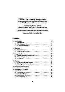
Response of the Mid latitude Ionosphere to Geomagnetic Storms The algorithm is further used to study the response of the mid-latitude ionosphere to geomagnetic storms of different strength. The data used for the study has been made available through the Internet by the International Ionospheric Tomography Community (IITC). TEC data are obtained at a chain of three receivers by monitoring Navy Navigational Satellite System (NNSS) satellite signals in the Alaskan region along 145oW longitude. The station coordinates are Cordova (60.495oN, 145.476oW), Gakona (62.399oN, 145.1570W) and Delta (63.902oN, 145.240oW). It must be noted that the error in F-region height estimation using such a short receiving aperture (~380 km) may be very large. In order to avoid this error a regularization profile has been incorporated with F-region height being calculated from International Reference Ionosphere 2001. The daily average Dst index varied from 0.04 nT to –73 nT during the period of the study. The days selected for the study are 23rd February, 14th July, 15th July, 16th July and 30th October, 2003 with mean Dst indices 4nT, -33nT, -42nT, -73nT and –235nT respectively. Fig.5 shows the scatter plot between the reconstructed foF2 and measured foF2 at Gakona for different days. The foF2 data from the ionosonde located at Gakona is available only for 23 February, 14 July, 15 July and some hours of 16 July. For 30 October, no ionosonde data are available. The plot shows that the reconstructions slightly underestimate the ionosonde value, but the correlation coefficient is very high (r2=0.86). It should be noted that the regularization profiles used in the reconstructions are simple Chapman profiles with the maximum electron density and the height of maximum ionization being obtained from the IRI-2001 model.
8
6
Ionosonde foF2 (MHz)
0.35 0.3
R 2 = 0.6867
11
-3
R2=0.86
Density gradient (10 m )
The density gradient in the pole ward edge of the trough seems to be correlated with the strength of geomagnetic storm. Fig.6 shows a plot of density gradient in the pole ward edge of the trough versus the variation of Dst index from the daily average values for all the days of high magnetic activity. The density gradient is normalized with respect to the density in the trough. The correlation between the two is very good (r2=0.6867). However, more reconstructions need to be performed for the generalization of such a correlation, as the data points are limited in our case. Kersley et al. [10] have shown that the density gradient in the pole ward edge of the trough increases with the increased magnetic activity characterized by Kp indices. It is to be noted that in the average behaviour, the gradients on both walls are often comparable in the daytime and evening for a given level of magnetic activity. Thus, the present observations are in agreement with the results of Kersley et al. [10].
4
2
0 0
2
4
6
8
Reconstructed f oF2 (MHz)
Fig. 5: Scatter plot between Reconstructed foF2 and Ionosonde foF2.
0.25 0.2 0.15 0.1 0.05 0 -200
-100
0
100
200
Variation of Dst index (nT) from daily mean
Fig. 6: Correlation between normalized density gradient in the pole ward edge of the trough and the Dst index.
DISCUSSION The GSVD algorithm eliminates the need for an initial guess to initiate the process of reconstruction. The large pointto-point oscillations that may occur in the solution can be avoided in this approach by incorporating regularization. The regularization can also be used for feeding the solver by a priori information on the electron density distribution. The reconstruction quality is very good when the data is free from noise and no regularization profile is needed. But, in presence of noise the reconstruction becomes completely useless unless a regularization profile is used to dampen the wild behaviour of the solution. The simulation studies of the trough models show that the algorithm is capable of reconstructing the position of the trough as well as the density gradient in the trough reasonably well. The very low values of the parameters ρ l 2 and ρ c for both the cases demonstrate the fact. Results indicate that this GSVD based CIT algorithm is capable of recreating the electron density distribution of the ionosphere satisfactorily even in the presence high level of noise. The comparison of reconstructed electron density distribution with ionosonde data shows that the algorithm is very much capable of reconstructing the midlatitude ionosphere. The reconstructed density values are somewhat lower than the ionosonde values, but the very strong correlation establishes the validity of the reconstruction results beyond doubt. Another advantage of the method has been its ability to reconstruct without the help of any initial guess regarding the state of the ionosphere in the region of interest. ACKNOWLEDGEMENTS This work is partially supported by the Indian Space Research Organization through the grant 10/2/258-NE. The IRI is a joint venture of the COSPAR and URSI. The authors are also thankful to the International Ionospheric Tomography Community for making the TEC data available in the Internet. REFERENCES [1]
J.R. Austen , S. J. Franke, and C. H. Liu, Ionospheric imaging using computerized tomography, Radio Sci., Vol.23(3), pp299-307, 1988. [2] J.R. Austen, S. J. Franke, C. H. Liu, and K. C. Yeh, Application of Computerized tomography techniques to ionospheric research, Radio beacon contribution to the study of ionisation and dynamics of the ionosphere and corrections to geodesy (Ed. A. Taurianen), Oulu, Finland, Part 1, pp25-35, 1986. [3] R. Leitinger, Ionospheric Tomography, Appeared as Chapter 24 in Review of Radio Science 1996-99, edited by Ross Stone, Oxford Science Publications, pp581-623, 1999. [4] K. Bhuyan, S. B. Singh, and P. K. Bhuyan, Application of Generalized Singular Value Decomposition to Ionospheric Tomography, Ann. Geophys., Vol.22, pp3437-3444, 2004. [5] K. Bhuyan, S. B. Singh, and P. K. Bhuyan, Tomographic reconstruction of the ionosphere using generalized singular value decomposition, Current Sci., Vol.76(7), pp1117-1120, 2002. [6] P.C. Hansen, Numerical tools for analysis and solution of Fredholm integral equation of the first kind, Inverse problems, Vol.8, pp849-872, 1992. [7] A.N. Tikhonov, Solution of incorrectly formulated problems and the regularization method, Soviet Math. Dokl., Vol.4, pp1035-1038, 1963. [8] P.C. Hansen, Rank-Defficient and Discrete Ill-posed Problems: Numerical Aspects of Linear Inversion, pp247, Society for Industrial and Applied Mathematics, Philadelphia, 1998. [9] E.S. Andreeva, V. E. Kunitsyn, and E. D. Tereshchenko, Phase-difference radio tomography of the ionosphere, Ann. Geophys., Vol.10, pp849-855, 1992. [10] L. Kersley, S. E. Pryse, I. K. Walker, J. A. T. Heaton, C. N. Mitchell, M. J. Williams, and C. A. Wilson, Imaging of electron density troughs by tomographic techniques, Radio Sci., Vol.32(4), pp1607-1621, 1997.