Application of Modified Gravitational Search Algorithm to Solve the

IJCSI International Journal of Computer Science Issues, Vol. 10, Issue 3, No 2, May 2013 ISSN (Print): 1694-0814 | ISSN (Online): 1694-0784 www.IJCSI.org

1

Application of Modified Gravitational Search Algorithm to Solve the Problem of Teaching Hidden Markov Model Ali Asghar Rahmani Hosseinabadi1, Mohammadreza Ramzannezhad Ghaleh2, Seyed Esmaeil Hashemi3

*

1

Young Research Club, Behshahr Branch, Islamic Azad University Behshahr, Iran Department of Computer, Behshahr Branch, Islamic Azad University Behshahr, Iran

2,3

Abstract Hidden Markov Model is a finite series of states that is continues with a probability distribution in a special state, an output can be obtained by continuous probability distribution. Since states are hidden from outside, this model is called Hidden Markov Model. In ordinary Markov Model, the position is directly visible to observer so probabilities transference state will be the only parameters. In Hidden Markov Model, the position is not visible directly but the affected variants by the position are visible. Each state taken for a possible output will have a probability distribution. Therefore, the sequence of taken states created by HMM would provide some information about the sequence state. Hidden Markov Models will be distinguished for their instruction in identifying the temporary patterns such as speech, handwriting, identifying hint and pointing, bioinformatics and so on. In this paper, a new method based on Modified Gravitational Search Algorithm (MGSA) has been used to improve the teaching of Hidden Markov Model (HMM). The teaching of HMM is based on Baum-Welch algorithm (BW). One of the problems of HMM teaching is the absence of any assurance about reaching of this algorithm to global optimum and the convergence of this method is often towards a local optimum. In this paper, the Modified Gravitational Search Algorithm has been used to exit Baum-Welch from local optimum and search for other optimal points. Furthermore, we have compared the proposed algorithm with two algorithms, PSO and Ant Colony, which have been used finally in Speech Recognition.

Keywords: Hidden Markov Model; Modified Gravitational Search Algorithm; Baum-Welch Algorithm; PSO Algorithm; Ant Colony Algorithm

1. Introduction The main idea of HMM theory was proposed about Speech Recognition in 1960s and has been applied well in its different problems [1]. HMM is one of the successful statistical methods in the field of Speech Recognition [2]. Many methods have been presented for HMM teaching up to now but more of them do not assure the convergence and reaching to the optimal point. One of these methods is Baum-Welch algorithm being presented for optimization of model parameters [3]. Baum-Welch has a high convergence speed and assures

after each repetition that the new model will operate better than previous model or its equivalent. However, Baum-Welch as a Hill Clamping method is sensitive to giving the initial values to model parameters and it often converge to local optimum. It may reduce the HMM power in classification or recognition of sequence [4]. In recent years, many algorithms have been proposed to meliorate the parameters of Hidden Markov Model. Some of these algorithms include: Tsong- Yi Chen et al. (2004) studied the problem of HMM optimization through Tabu Search Algorithm with the purpose of melioration, finding model optimal parameters, and searching for HMM ideal parameter structure in automatic Speech Recognition [5]. Y. Fengquin and Z. Changhai (2008) used the combinational algorithm of PSO with Baum-Welch to teach continuous HMM that the obtained results of this combinational algorithm are indicative of the system operation melioration to GA algorithm [6]. Jun Meng et al. (2010) studied the problem of teaching DHMM based on several program forms and its usage in sequences classification. To do this they used PSO algorithm to eliminate BW faults and to reach the global optimum that the results of this action will be beneficial in meliorating the average probability and accuracy in classification [4]. In this paper, a method based on Modified Gravitational Search Algorithm (MGSA) has been used to solve the problem of teaching Hidden Markov Model [7, 8]. In proposed algorithm, a method has been created by using the gravity law to find optimum. In above algorithm, a set of bodies will search the space at random. The gravity law has been used as an instrument to exchange information. Each body reaches to an approximate perception of its surrounding space through the effect of other bodies’ force. The algorithm is guided so that the position of bodies will meliorate by passing the time. To do this, inertia and gravity masses are regulated. According to relations, all bodies influence on each other somewhat and their effect on neighbor bodies will be more. The effect of heavier bodies is more and they have a bigger effective radius. Therefore, more gravity mass is

Copyright (c) 2013 International Journal of Computer Science Issues. All Rights Reserved.


attributed to those bodies having better fitness function. As a result, bodies will be guided towards better positions by passing the time [7]. The aim of this paper will be comparison of combinational methods; including PSOBW, Ant Colony BW, and MGSABW; to optimize continuous HMM parameters and comparison of these method’ capabilities in Speech Recognition to BW method. The structure of this paper is as the following: In section 2, Hidden Markov Model and BW method will be explained generally. Section 3 explains the theory of MGSA method. The details of combinational algorithm will be studied in section 4. The application of combinational method and the results of its tests on presented data have been displayed in section 5 and finally, section 6 includes conclusion.

2. Hidden Markov Model and its teaching by Baum-Welch Hidden Markov Model is a probability model, which is used to display statistical features of random processes and will be described by model parameters. The random process in Speech Recognition includes random sequences with given length called observation symbols and will be displayed by . In which M is the dimension of observation symbol. A Discontinuous Hidden Markov Model (DHMM) having N states of can be determined by triplet set of λ= (A, B, π). In which: A: is the probability distribution of initial state and is used to display the initial probability distribution of state at the time t=1. It will be obtained by equation (1):

  P(q1  Si )

i  1,2,...N

(1)

2

This must make the equation (4): M

a i 1

ij

1

(4)

{ } is the | C: observations probability matrix in discontinuous HMM. The element of ith row and kth column is bik of observation symbol probability and index i will be indicative of ith state, which must make equation (5): M

 b (k )  1 i 1

(5)

i

If the observations are continuous, a function of continuous probability density must be used instead of discontinuous probabilities. The probability density will be usually calculated with the aid of a weighted set of normal distribution M of R that is displayed by equation (6): M





b j (O)   c jm R O,  jm ,U jm 1  j  N

(6)

m 1

Where is the constant of mth normal distribution at state j , R is usually the Gaussian function with average vector and covariance matrix is for mth normal distribution. constant must make equations (7) and (8): M

C m 1

jm

 1,

C jm  0,

1 j  N

1  j  N ,1  m  M

(7)

(8)

This must make equation (2): N

 i  1

(2)

i 1

B: { | } is the transference probability matrix between states. The element of ith row and jth column is probability or the transference probability from current state i to next state j that is calculated by equation (3):

aij  P(qi  S j qi 1  S i ),

(3)

This method is used in Continuous Hidden Markov Model (CHMM). A Hidden Markov Model with continuous probability distribution will be displayed by equation (9) too:

  ( A, c jm ,  jm ,U jm ,  )

(9)

In teaching process, an observation vector in length T such as { } and an initial λ model are given. The aim of teaching how to evaluate



parameters is to maximize the similarity criterion (ML) | . of this observation that is to increase In traditional BW method, a new model is obtained | | . This after each repetition, so that process will be repeated until the probability increases. BW algorithm has a high convergence speed but the result of optimization by this algorithm depends on the initial model and usually will be trapped in a local optimum [3]. In this paper, we will focus on the problem of how to obtain model parameters to increase the amount of | probability. For this purpose, the GSABW combinational method has been presented and used in above paper.

3. GSA Algorithm 3.1 Main idea To suppose the problem search space (circumference) as a multidimensional coordinate system in which there are some solutions to solve the considered problem. Each point of space is a solution of the problem. Each solution has a mass which is calculated by the goal function related to that mass. The better the solution is, the more values are produced by the goal function and as a result, its mass would become more. Furthermore, researcher agents are a set of bodies. After the formation of research space, its governed rules are specified. It is supposed that just gravity and motion laws govern [9-12]. Gravity law: each body in research space magnetizes all other bodies towards itself. The amount of this force is proportional to the gravity mass of that body and to the reverse of distance between those two bodies. Motion laws: The current speed of each body equals to the sum of a coefficient of body’s previous speed and its speed change. The speed change or velocity of each body also equals to the force upon that body divided to gravity mass [11].

3.2 Modified Gravitational Search Algorithm In GSA algorithm, which is created based on gravity law between Newton bodies, each body will have four features including [7]: Position, inertia mass, active gravity mass and passive gravity mass. The position of a body is accordant to the answer of problem, the inertia and gravity masses are specified by evaluation function. Now, consider a system with N agents (bodies). The position of each body in search space is a point of that space which will be taken in to account as a solution to the problem. This position is obtained by equation (10) in which the dimension d of body i has been displayed by .

3

xi  ( xiI ,..., xid ,...xin ) i  1,2,..., N

(10)

In this system, a force equal to is imposed from body i at the time t and at the dimension d to each body j. The amount of this force will be calculated by equation (11):

Fijd (t )  G(t )

M pi (t )  M aj (t ) Rij (i)  

( xid (t )  xid (t )), (11)

Where is the active gravity mass related to j th agent, is the passive gravity mass related to ith agent, G(t) is the gravity constant at time t, ε is a small constant, and is the Euclidean distance between two agents i and j.

Rij (t )  X i (t )  X j (t )

(12)

2

on body i at the direction of The imposed force dimension d and at time t is a sum of dth dimension of imposed force from other agents so that this sum has been weighted randomly and is obtained by equation (13):

Fi d (t ) 

 w( j)  F

jKbest, j  i

d ij

(t )

(13)

Kbest is a K agent set which should have the best fitness and heaviest mass, and w (j) is weight coefficient that will be obtained by equation (14):

w( j )  ( wini  wend ).

k best  j  wend k best

(14)

Furthermore, the velocity of agent i at the time t and at dimension d, , is calculated by equation (15):

aid (t ) 

Fi d , M n (t )

(15)

Where is the inertia mass of agent i. Thus the next speed of each agent will become as the sum of a fraction of its present speed and velocity. So, the speed and position of agent are calculated by equations (16) and (17):



xid (t  1)  xid (t )  vid (t  1)

(16)

vid (t  1)randi  vid (i)  aid (t )

(17)

Where is a steady random coefficient in range (0,1). This random number will be used to give a random feature to the search. Gravity constant G is given initial value and will reduce by passing the time to control the accuracy of search. In other words, G is a function of initial value G0 and time: G(t )  G(t , G0) Inertia and gravity masses are calculated easily from fitness function. The heavier mass is related to more effective agen. That is, better agents will have more magnetism and less speed. On the supposition that the inertia and gravity masses are equal, the values of masses are calculated using fitness function. The inertia and gravity masses will be updated by equations (18) and (19):

M ai  M pi  M ii  M i , M i (t ) 

fit i (t )  worst(t ) , best (t )  worst(t )

i  1,2,..., N ,

4

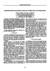
Generate initial population

Evaluate the fitness for each agent

Update the G, best and worst of the population

Calculate M and a for each agent

Update velocity and position

NO

Meeting end of criterion?

(18) YES (19) Return best solution

is the fitness value of agent i at the time t. worst(t) and best(t) are determined by equations (20) and (21): Fig. 1 levels of gravity force algorithm [12]

best (t )  max fit j (t )

(20)

worst(t )  min fit j (t )

(21)

j1,...N 

j1,...N 

Since there will be the possibility of catching in local minimum at high repetitions, so we can use the spring operator to escape from local minimum. So that, if we have the same optimal answer in several successive repetitions, we make a change in existent population by applying the spring action to exit it from local optimum.

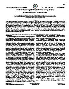
4. Proposed algorithm In this paper, a combination of two algorithms, MGSA and BW, has been used to teach Markov Model. The levels of the above combinational algorithm have been organized as following to solve the considered problem:

A: Giving the initial value to agents Markov Model parameters must be given initial value in MGSABW software. In MGSA algorithm, the position of objects including:

X i  ( xi1 ,...xid ,..., xin )

i  1,2,...N

Vi  (vi1 ,...vid ,...vin )



And their speed is the criterion of action. So ,at first their value is chosen randomly and then we will normalize X values to provide HMM conditions. The length of X vector depends on the values of parameters A and B and will be composed of a string of random real numbers as shown in figure (2). In figure (2), A is the transference matrix, bm is the average values of normal distributions, and bv is their variance values. Also, N and M will respectively the number of states and the number of observation symbols at each state.

B: Evaluating the fitness and stop condition The fitness value of each agent is obtained by calculating | by forward–backward algorithm [13, 14] and fitness function is calculated by equation (22):

f ( xi )  log P(O  ) 

1 L log P(O l  )  L l 1

Fig. 3 Levels of proposed algorithm

Where will be the sequence of 1 observations. Stop condition can be the maximum of algorithm repetition or this process would continue until f(x(t)) - f(x(t-1)) < ε .

C: Updating the speed and position After evaluation of F, M and a by equations (13), (19) and (15), the speed and position of body are calculated by equations (16) and (17). After each repetition of MGSA algorithm, the values are given to BW algorithm and then BW will evaluate these values. Levels of proposed algorithm have been displayed completely in figure (3).

A a11

B (means) a NN

bm11

...

bm1M

...

bmNM

bv11

...

1. Determining the circumference of system and giving the initial value to X and V populations 2. Arranging the solutions based on their mass 3. Choosing the first solution as the best one 4. Evaluation of bodies 5. Calculating the fitness of each person using forward-backward algorithm 6. Calculating G 7. Calculating the imposed gravity force on each body 8. Updating G, the best and the worst person 9. Implementing BW algorithm for each agent 10. Calculating M and a for each agent 11. Updating V speed and X position 12. Displacing the solutions at each dimension based on the force being imposed on them in different dimensions 13. Has the stop condition been made? 14. Convert the best solution else step 2

(22)

th

...

5

Table 1: The probability logarithm of having been thought models by four different methods Models

BW

Sil

-668.6604

W

-870.2077

a

Ant Colony

PSOBW

MGSABW

-668.6508

-668.4007

-668.4004

-870.2075

-870.2077

-870.2077

-845.9854

-845.9861

-845.9859

-845.9853

n

-1022.2240

-1022/1420

-1022.1421

-1022.1416

t

-815.4918

-815/4619

-815.3989

-815.4015

u

-1492.2116

-1492/2134

-1492.2126

-1492.2115

th

-798.0760

-798/0783

-798.0779

-798.0760

BW

r

-983.5443

-983/5512

-938.5501

-983.5432

i

-1332.5593

-1332/6101

-1332.5912

-1332.5589

f

-802.7164

-802/7165

-802.7164

-802.7162

o

-974.9783

-974/9774

-974.9771

-974.9770

῀i

-731.7753

-731/7750

-731.7753

-721.6470

B (Variance)

v

-986.9370

-986/9122

-986.8986

-986.8984

...

s

-1289.2093

-1283/0167

-1283.0058

-1283.0060

bv1M

Fig. 2 Structure of chromosome (HMM parameters)

bvNM

e

-634.0833

-634/0829

-634.0832

-634.0832

k

-1039.1685

-1039/1682

-1039.1685

-1039.1459

y

-824.3581

-824/3671

-823.8236

-823.8237



5. The results of simulation In this paper, an instrument called HTK has been used to create Hidden Markov Model. HTK is a software which has been developed to create Hidden Markov Model and it will be used to Speech Recognition too [15]. In above paper, we will use Hidden Markov Model having five-left- to- right states. A Gaussian normal distribution with 39 dimensions has been considered inside each state because observations vector is a 39 dimensional vector. The applied data are English numbers 1 to 9 saved independently from speaker (different 5 men and women). Each number has been repeated 5 times and totally will include 270 words. 70% of the whole data have been considered for teaching and 30% for testing. It means that, 21 data for teaching and 9 data for testing have been considered from each number. The extracted features include 13 Mel Frequency Cepstral Coefficients (MFCC) along with their derivatives; as a result, 39 features have been extracted for each speech frame. The length of string for position of each body has been considered 240 numbers. Since the left-to-right Hidden Markov Model has been used, just 6 elements of transference matrix change. Therefore, we devote 6 first numbers of the string to the transference matrix and the values of other elements have been considered according to figure (2). Four algorithms including BW, PSOBW, Ant Colony BW and MGSABW have been used in phoneme identification. The number of BW algorithm repetition in all four methods has been considered as 20 and this number for PSO, Ant Colony, and MGSA is equal to 25 too. The number of population in all three combinational algorithms has been considered equal to 20. The value of spring probability for spring action in MGSABW algorithm is equal to 0.8 and the spring is done just for a number from a 240 string. From the set of English numbers 1 to 9, 17 phonemes along with silent were extracted so one HMM was considered for each phoneme. The obtained results of teaching each phoneme along with the value of Maximum Likelihood, which must be minimized, has been presented in table (1). Concerning table (1), the proposed algorithm in most of the cases will operate better than BW or PSOBW and Ant Colony BW methods and will reach to a less minimum than the three above methods. The amount of three methods’ efficiency in phoneme identification has been studied in table (2). Two sets have been considered to test the models. The first set is teaching data and all four models have been taught by these data. The obtained results of them are visible in table (2) about all four models.

6

As it is visible in table (2), the amount of phoneme identification by MGSABW method has been optimized about 0.48% in comparison to BW method and it has had a superiority to Ant Colony and PSOBW methods, respectively about 0.19% and 0.23%. The second set of testing data, has been considered out of teaching data range. The obtained results of this set will be visible in table (3). Concerning table (3), it can be seen that MGSABW model has operated much better than BW and Ant Colony BW models and has reached melioration in identification to these two models, respectively about 0.44% and 0.48% it also has had a melioration about 0.36% to PSOBW model. Table 2: The amount of identification for the first set of data

BW

Percentage of

Ant Colony BW

95.03

PSOBW

MGSABW

95.32

95.51

phoneme identification Correct phoneme Replaced phoneme Deleted phoneme Added phoneme Total phonemes

995

996

998

1000

15

15

14

14

37

36

35

33

11

11

11

11

1047

1047

1047

1047

Table 3: The amount of identification for the second set of data

BW

Percentage of

Ant Colony BW

96.00

PSOBW

MGSABW

96.44

96.44

phoneme identification Correct phoneme Replaced phoneme Deleted phoneme Added phoneme Total phonemes

432

433

433

433

8

8

7

7

10

9

9

9

4

5

5

5

450

450

450

450



6. Conclusion

[9]

In this paper, a combinational algorithm called MGSABW was used to solve the problem of teaching Hidden Markov Model and meliorating the HMM model parameters. The obtained results of this algorithm were compared to BW method and to combinational methods including PSOBW and Ant Colony BW. Theoretically, the complementary methods such as PSO and MGSA can reach to global optimum or to its approximation and the amount of this melioration will be more obvious in great systems. The obtained results of the above tests show that MGSABW algorithm operates better than BW, PSOBW, and Ant Colony BW algorithms. These results will be also indicative of models melioration by MGSABW algorithm to BW method, about 0.44% for testing data out of teaching data. Concerning the above results, it is clear that this method can be an appropriate replacement to gain a better answer in calculation of Markov Model parameters, too.

References [1]

H. Sajedi et al, “A Grouping-based method for On-Line Persian Discrete Character Recognition Using Hidden Markov Model,” International Conference of Computer Society of Iran, Tehran, Iran, 2007, 419-426.

[2]

L. R. Rabiner, “A tutorial on hidden Markov models and selected applications in speech recognition,” In Proceedings of the IEEE, Vol. 77(2), 1989, pp. 257-285.

[3]

L. Xue, J. Yin and Z. J. Lai Jiang, “A Particle Swarm Optimization for Hidden Markov Model Training,” International Conference on Signal Processing, 2006, 16-20.

[4]

J. Meng et al, "Swarm-based DHMM Training and Application in Time Sequences Classification", Journal of Computational Information Systems, Vol. 6(1), 2010, pp. 197-203.

[5]

T. Chen, X. Mei and J. Pan and S. Sun, “Optimization of HMM by the Tabu Search Algorithm,” Journal of Information Science and Engineering, Vol. 20, 2004, pp. 949-957.

[6]

Y. Fengqin, Z. Changhai, “An Effective Hybrid Optimization Algorithm for HMM,” Proceedings of the Fourth International Conference on Natural Computation, icnc, 2008, pp. 80-84.

[7]

E. Rashedi, H. Nezamabadi-pour and S. Saryazdi, “GSA: A Gravitational Search Algorithm,” Information Sciences, Vol. 179, 2009, pp. 2232–2248,.

[8]

E. Rashedi, H. Nezamabadi-pour and S. Saryazdi, “BGSA: binary gravitational search algorithm,” Springer Science Media, Vol. 9, 2009, pp. 727-745.

7

B. Webster and J. B. Philip, “A Local Search Optimization Algorithm Based on Natural Principles of Gravitation,” Proceedings of the International Conference on Information and Knowledge Engineering, Vol. 1, 2003, 255-261.

[10] A. S. Rostami, H. M.Bernety and A. R. Hosseinabadi, “A Novel and Optimized Algorithm to Select Monitoring Sensors by GSA,” ICCIA, 2011, 829–834. [11] A. R. Hosseinabadi, M. Yazdanpanah and A. S. Rostami, ”New Search Algorithm for Solving Symmetric Traveling Salesman Problem Based on Gravity,” World Applied Sciences Journal, Vol. 16 (10), 2012, 1387-139. [12] Ali Asghar Rahmani Hosseinabadi, Abbas Bagherian Farahabadi, Mohammad Hossein Shokouhi Rostami, Ahmad Farzaneh Lateran, “Presentation of a New and Beneficial Method Through Problem Solving Timing of Open Shop by Random Algorithm Gravitational Emulation Local Search,” International Journal of Computer Science Issues, Vol. 10, Issue 1, 2013, 745-752. [13] Gary D. Brushe, Robert E. Mahony and John B. Moore, “A Forward Backward Algorithm for ml state and sequence estimation,” International Symposium on Signal Processing and its Applications, ISSPA, Gold Coast, 1996, Australia, 25-30 August. [14] Shun-Zheng Yu, Hisashi Kobayashi, “An Efficient Forward–Backward Algorithm for an Explicit-Duration Hidden Markov Model,” IEEE Signal Processing Letters, Vol. 10, 2003, 11-14. [15] J. Picone, “Continuous speech recognition using hidden Markov models,” IEEE ASSP Magazine, Vol. 7, 1990, pp. 26-41.

Ali Asghar Rahmani Hosseinabadi Bachelor of Computer - Software Trends, Islamic Azad University, Science & Research Amol 2010. Elite Member of the National Foundation of Young Researchers Club, Islamic Azad University, Behshahr Center. His Areas of research: intelligent and innovative Optimization Algorithms are used, Scheduling Flexible Manufacturing Systems, Image Processing, Intelligent Routing, Tsp, Vrp, Time Tabeling, Wireless sensor networks.



Mohammadreza Ramzannezhad Ghaleh Computer Sc - Software Engineering Trends, Islamic Azad University, Bushehr Science Research 2012. Mazandaran University Lecturer of Islamic Azad University, Behshahr Branch, His Areas of research: intelligent and innovative Optimization Algorithms are used, Tsp, Vrp.

Seyed Esmaeil Hashemi Computer Sc - Software Engineering Trends, Islamic Azad University, Sari Science Research 2013. Mazandaran University Lecturer of Islamic Azad University, Behshahr Branch, His Areas of research: intelligent and innovative Optimization Algorithms are used, Data mining.


8