SUPPLEMENTARY INFORMATION
Application of Multivariate Multiple Regression and Design of Experiment for Modelling the Effect of Monoethylene Glycol in the Calcium Carbonate Scaling Process Vinicius Kartnaller1, Fabrício Venâncio1, Francisca F. do Rosário2 and João Cajaiba1,* Universidade Federal do Rio de Janeiro (UFRJ), Instituto de Química, Pólo de Xistoquímica, Rua Hélio de Almeida 40, Cidade Universitária, Rio de Janeiro, 21941-614, Brazil. 2 Centro de Pesquisas e Desenvolvimento Leopoldo Américo Miguez de Mello, PETROBRAS, Cidade Universitária, Rio de Janeiro 21040-000, Brazil. * Correspondence:
[email protected]; Tel.: +55-21-2562-5323 1
Academic Editor: name Received: date; Accepted: date; Published: date
1. Introduction In this supporting information, results regarding the regression models will be displayed. Even though the methods are common and basic in the statistics area, in order for a better understanding, a quick review regarding the statistical tests to evaluate any regression model will be given. We encourage the reader to consult other references for a deeper view of the methods discussed here. 1.1. Analysis of Variance (ANOVA) Having been made a regression model, it is necessary to verify if there is a good fit between it and the experimental data. One of the most used method is the Analysis of Variance (ANOVA). In ANOVA, the variability of the experimental data is divided into two components: • Sum of Squares of the Regression (SSR) - measures the amount of variability explained by the regression model; • Sum of Squares of the Error (SSE) - measures the residual variation that is not explained by the independent variables; We can then write the total variability of the experimental data as the Total Sum of Squares (SST) as in Equation (S1): 𝑆𝑆𝑇 = ∑ 𝑦𝑖2 −
(∑ 𝑦𝑖 )2 𝑁
= 𝑆𝑆𝑅 + 𝑆𝑆𝐸
(S1)
where 𝑦𝑖 is the i-th value of the dependent variable dataset and N is the number of experiments performed and used in the regression. The SST is correlated to how the experimental values (of the dependent variable) vary in respect to their mean value. Regarding the degree of freedom for each of the sums described, one can initially assume that the entire modelling has (N - 1) degrees of freedom. Hence, the SST has (N - 1) degrees of freedom. By doing the regression, p degrees are used for the estimation of the unknown coefficients (b1, b2, ..., bp), where the linear coefficient b0 is not considered a regressor since it is a function of other estimates. In this case, p is the total number of independent variables used in the mathematical model. Hence, the SSR has p degrees
of freedom. Since SST = SSR + SSE, then it can be found that the SSE has (N - p - 1) degrees of freedom. The SSE deals with the variability not explained by the regression, and can be defined as: 𝑆𝑆𝐸 = ∑(𝑦𝑖 − 𝑦̂𝑖 )2
(S2)
where 𝑦̂𝑖 is the value predicted for the dependent variable by the model for the i-th sample. The SSR relates the modelled data to the mean value of the dependent variable, and can be defined as: 𝑆𝑆𝑅 = ∑ 𝑦𝑖2 −
(∑ ̂) 𝑦𝑖 2
(S3)
𝑁
The sum of squares can be viewed as variances for comparison amongst themselves, by dividing them by their degrees of freedom. This leads to the mean squares (MS) values: 𝑀𝑆𝐸 =
𝑆𝑆𝐸
(S4)
𝑁−𝑝−1
𝑀𝑆𝑅 =
𝑆𝑆𝑅
(S5)
𝑝
In addition, when one has a data set with replicates, in which variance can be estimated, one can partition the SSE into two components: one related to the pure error of the system and another associated with the lack of fit of the proposed mathematical model to the experimental points. The sum of squares related to the pure error (SSPE) can be written according to Equation (S6): 𝑛𝑗
𝑆𝑆𝑃𝐸 = ∑𝑐𝑗=1 ∑𝑖=1(𝑦𝑖𝑗 − 𝑦̅𝑗 )2
(S6)
In the equation, 𝑛𝑗 is the number of replicates of the same point and 𝑐 is the number of points in the set containing replicates. The value of SSPE is related to the experimental variance itself measured over the points in replicates, and no information of the regression is used for its calculation. In the case of design of experiments with replicates at the central point, we have N total experiments performed, where (𝑛𝑗 - 1) are repetitions of the same point. Hence, there are only m different experiments. In this case, the SSPE has a degree of freedom equal to (N - m). Since the SSE is partitioned into the sum of squares of the pure error and of the lack of fit (SSLF), the latter can be found from Equations (S2) and (S6): 𝑆𝑆𝐿𝐹 = 𝑆𝑆𝐸 − 𝑆𝑆𝑃𝐸
(S7)
In this case, the degrees of freedom for the SSLF can be found as (m - p - 1). Table S1 summarizes the ANOVA calculations. Table S1. Summary of the variation source for the ANOVA, the notations, degrees of freedom and significance tests
Variation Source Sum of Squares
Degrees of Freedom
Mean Squares
F0
Regression
SSR
p
MSR
MSR/MSE
Error
SSE
N-p-1
MSE
(Lack of Fit)
SSLF
m-p-1
MSLF
(Pure Error)
SSPE
N-m
MSPE
Total
SST
N-1
MSLF/MSPE
1.2. F-Test to Evaluate the Significance of the Regression The ANOVA F-test for the regression serves to check if the proposed model, which uses information from the predictor variables, is substantially better than a simple predictor: the mean value of the answers, 𝑦̅, which does not depend on any of these vari. For this, a hypothesis test is used, where: 𝐻0 : 𝑏1 = 𝑏2 = ⋯ = 𝑏𝑝 = 0 𝐻𝑎 : At least one of the coefficients 𝑏1 , 𝑏2 , ⋯ , 𝑏𝑝 is not zero The F-value can be found by the ratio between the mean squares of the regression and of the error, which has an F-distribution: 𝐹=
𝑀𝑆𝑅 𝑀𝑆𝐸
(S8)
The F-value can be compared to a tabled value, Fcrit, with degrees of freedom relative to that of the regression and that of the error, in that order. If F > Fcrit, the null hypothesis is not valid. Therefore, there is a correlation between the response and some of the coefficients, so that one can declare that the regression is significant. 1.3. F-Test to Assess Lack of Fit The F-test to verify the lack of fit must be performed in order to evaluate if the mathematical model proposed to respond to the experimental variability is adequate. The initial assumption is that the response could be described using the model that follows: 𝒚 = 𝒃𝑿 + 𝜺
(S9)
where 𝑿 is the design matrix, 𝒃 is the vector containing the coefficients and 𝜺 is the error vector. However, the real model describing the experimental variability is described by: 𝒚 = 𝒃𝑿 + 𝒃𝟐 𝑿𝟐 + 𝜺
(S10)
Thus, the estimate of the coefficients of the proposed model leads to inflated and biased values when the model does not fit well and 𝒃𝟐 ≠ 0. The hypothesis test for this evaluation is described by: 𝐻0 : 𝒃𝟐 = 0 𝐻𝑎 : 𝒃𝟐 ≠ 0 The F-value can be found by the ratio between the mean squares of the lack of fit and of the pure error, which has an F-distribution: 𝐹=
𝑀𝑆𝐿𝐹 𝑀𝑆𝑃𝐸
(S11)
The F-value can be compared to a tabled value, Fcrit, with degrees of freedom relative to the lack of fit and the pure error, in that order. If F < Fcrit, the null hypothesis is valid. Therefore, it can be said that the estimated coefficients are not biased and that there is a good fit between the mathematical model and the response. 1.4. Coefficient of Determination The coefficient of determination, also well known as R2, is a statistical measure of the strength of a regression model according to the total variability explained by it. It is defined as the ratio of the sum of squares of the regression in relation to the total sum of squares: 𝑅2 =
𝑆𝑆𝑅 𝑆𝑆𝑇
(S12)
Since the R2 value always increases as a new variable is added to a model, this value can be inflated artificially with the inclusion of more and more predictor variables, and then pass a false image on the actual fit of the model with such variables. For this, it can defined an adjusted coefficient of determination by dividing the sum of squares by their corresponding degree of freedom: 𝑅2 (𝑎𝑑𝑗. ) =
𝑀𝑆𝑅
(S13)
𝑆𝑆𝑇 ⁄(𝑁−1)
2. Methodology The applied design of experiments used was a 2 5-1 rotational central composite design, which design can be divided into three experimental portions: (1) factorial points, (2) central points, and (3) star points. The factorial portion was indeed a fractional factorial design with resolution V, meaning that all two factor interactions were aliased with three factor interactions. The central points were replicated six times. The star portion were made in order that the model would be rotational. Hence, α was chosen for this type of 2 5-1 design. Table S2 shows the coded design matrix and Table S3 shows the information of the factors, and their intervals.
Star Points
Central Points
Factorial Points
Table S2. Design matrix of the coded factors for the 2 5-1 rotational central composite design Experiment # 1 2 3 4 5 6 7 8 9 10 11 12 13 14 15 16 17 18 19 20 21 22 23 24 25 26 27 28 29 30 31 32
Pressure (X1) -1 1 -1 1 -1 1 -1 1 -1 1 -1 1 -1 1 -1 1 0 0 0 0 0 0 -2.378 2.378 0 0 0 0 0 0 0 0
Temperature (X2) -1 -1 1 1 -1 -1 1 1 -1 -1 1 1 -1 -1 1 1 0 0 0 0 0 0 0 0 -2.378 2.378 0 0 0 0 0 0
MEG Conc. (X3) -1 -1 -1 -1 1 1 1 1 -1 -1 -1 -1 1 1 1 1 0 0 0 0 0 0 0 0 0 0 -2.378 2.378 0 0 0 0
Bicarbonate Conc. (X4) -1 -1 -1 -1 -1 -1 -1 -1 1 1 1 1 1 1 1 1 0 0 0 0 0 0 0 0 0 0 0 0 -2.378 2.378 0 0
Calcium Conc. (X5) 1 -1 -1 1 -1 1 1 -1 -1 1 1 -1 1 -1 -1 1 0 0 0 0 0 0 0 0 0 0 0 0 0 0 -2.378 2.378
Table S3. Summary of the factors studied in the design of experiments. with their different levels studied for the modelling levels -2.378
-1
0
1
2.378
X1: Pressure (psi)
0
714
1233
1751
2466
X2: Temperature (°C)
40
60
75
90
110
X3: MEG Conc. (%)
0
23
40
57
80
X4: Bicarbonate Conc. (ppm)
1000
2449
3500
4551
6000
X5: Calcium Conc. (ppm)
1000
2449
3500
4551
6000
3. Results 3.1. Response Matrix Used for the Modelling The response matrix is presented at Table S4, where the scaling time, in seconds, is shown for the 32 central composite experiments. Each experiment shows 25 datapoints, corresponding to the 25 different models being constructed. It is worth remembering that the models are referenced to the advancement of the scaling process, and are related to how the differential pressure signal increases as deposition occurs in the tube line. Hence, Model 1 is the scaling time so that the baseline increases 1 psi; Model 2 is the scaling time so that the baseline increases 2 psi; and so on, until Model 25, which is the scaling time so that the baseline increases 25 psi. 3.2. Modelling of the Data Using the Scaling Time Directly The first model tested was using the scaling time (𝑡𝑠𝑐 ) directly, using Equation 5 of the manuscript. However, variables (𝑏1 , 𝑏12 , 𝑏11 , and 𝑏55 ) did not show significance and were eliminated from the model. The final model was then: 𝑡𝑠𝑐 = 𝑏0 + (𝑏2 × 𝑇) + (𝑏3 × 𝑀𝐸𝐺) + (𝑏4 × 𝐶𝐻𝐶𝑂3 − ) + (𝑏5 × 𝐶𝐶𝑎2+ ) + (𝑏13 × 𝑃 × 𝑀𝐸𝐺) + (𝑏14 × 𝑃 × 𝐶𝐻𝐶𝑂3 − ) + (𝑏15 × 𝑃 × 𝐶𝐶𝑎2+ ) + (𝑏23 × 𝑇 × 𝑀𝐸𝐺) + (𝑏24 × 𝑇 × 𝐶𝐻𝐶𝑂3 − ) + (𝑏25 × 𝑃 × 𝐶𝐶𝑎2+ ) + (𝑏34 × 𝑀𝐸𝐺 × 𝐶𝐻𝐶𝑂3 − ) + (𝑏35 × 𝑀𝐸𝐺 × 𝐶𝐶𝑎2+ ) + (𝑏45 × 𝐶𝐻𝐶𝑂3 − × 𝐶𝐶𝑎2+ ) + (𝑏22 × 𝑇 × 𝑇) + (𝑏33 × 𝑀𝐸𝐺 × 𝑀𝐸𝐺) + (𝑏44 × 𝐶𝐻𝐶𝑂3 − × 𝐶𝐻𝐶𝑂3 − ) The ANOVA results for the modelling using this equation are presented in Table S5, the calculated coefficients are presented in Table S6 and the p-value for these coefficients are shown in Table S7.
Table S4. Response matrix showing the measured scaling time (in seconds) for the different experiments in the central composite design for the different models constructed Model Number Experiment #
1
2
3
4
5
6
7
8
9
10
11
12
13
14
15
16
17
18
19
20
21
22
23
24
25
1
1387
1444
1470
1487
1497
1504
1510
1514
1518
1520
1522
1524
1526
1528
1529
1531
1532
1533
1534
1535
1536
1537
1538
1538
1539
2
1728
1862
1917
1948
1968
1983
1996
2004
2011
2016
2021
2025
2029
2032
2035
2038
2041
2043
2045
2047
2049
2051
2052
2054
2055
3
431
434
436
437
438
439
440
440
441
441
442
442
442
443
443
443
444
444
444
444
444
445
445
445
445
4
379
423
432
434
436
437
438
439
439
440
440
440
441
441
441
442
442
442
443
443
443
443
443
444
444
5
2506
2690
2752
2782
2799
2811
2820
2828
2834
2839
2843
2847
2850
2853
2856
2859
2861
2864
2866
2868
2869
2871
2872
2874
2876
6
1937
1994
2038
2066
2080
2091
2099
2107
2116
2124
2131
2137
2142
2147
2151
2154
2157
2160
2162
2164
2168
2170
2173
2174
2176
7
1265
1374
1423
1452
1475
1493
1505
1519
1529
1536
1545
1553
1559
1564
1570
1574
1576
1589
1592
1594
1599
1601
1603
1605
1607
8
1270
1363
1412
1443
1458
1474
1485
1494
1501
1507
1512
1516
1520
1524
1526
1529
1531
1533
1535
1537
1538
1540
1541
1542
1543
9
865
900
917
931
942
950
955
960
964
967
970
972
973
975
976
978
979
980
981
982
983
984
985
985
986
10
957
984
996
1003
1008
1012
1014
1017
1018
1020
1021
1022
1023
1024
1025
1026
1026
1027
1028
1028
1029
1029
1030
1030
1030
11
452
458
460
461
462
463
464
464
465
465
466
466
466
467
467
467
467
468
468
468
468
468
468
469
469
12
397
403
405
407
408
408
409
409
410
410
411
411
411
412
412
412
412
412
413
413
413
413
413
413
414
13
2826
3204
3326
3394
3418
3473
3488
3497
3502
3507
3510
3514
3518
3521
3523
3525
3526
3528
3529
3530
3531
3532
3533
3534
3535
14
2810
3245
3478
3623
3729
3811
3876
3924
3962
3998
4020
4033
4045
4055
4069
4116
4127
4136
4145
4153
4159
4165
4172
4188
4194
15
1084
1128
1167
1193
1216
1224
1237
1243
1262
1273
1284
1306
1308
1320
1335
1344
1349
1361
1369
1381
1378
1380
1381
1381
1382
16
1137
1218
1250
1281
1292
1305
1309
1312
1325
1328
1330
1340
1342
1343
1345
1346
1348
1349
1351
1353
1355
1357
1358
1360
1361
17
640
658
667
672
677
680
683
685
686
688
689
691
692
694
695
697
698
699
700
701
701
702
703
703
704
18
735
758
768
775
780
784
787
790
792
795
797
798
800
802
803
804
806
807
808
809
810
811
811
812
813
19
670
682
688
692
695
696
698
699
700
701
702
703
705
706
706
707
708
709
709
710
710
711
711
711
712
20
741
766
775
779
782
785
786
788
790
791
792
793
794
796
797
798
799
799
800
800
800
801
801
801
802
21
767
781
785
788
791
793
794
795
798
799
800
802
802
803
804
805
805
806
807
807
808
808
809
809
809
22
675
688
695
698
699
701
702
703
704
704
705
706
706
707
708
708
709
709
709
710
710
711
711
711
712
23
730
791
820
836
847
857
865
871
876
880
884
887
891
893
896
898
901
903
904
906
908
910
911
912
914
24
738
759
769
774
777
780
782
784
786
788
789
790
792
793
793
794
795
795
796
797
797
798
798
799
799
25
5922
6197
6276
6322
6353
6377
6399
6417
6432
6445
6456
6467
6477
6485
6494
6501
6508
6514
6519
6525
6530
6533
6538
6542
6545
26
642
651
653
654
655
656
656
657
658
658
658
662
665
665
666
666
666
666
667
667
667
667
667
668
668
27
613
631
638
642
644
647
648
650
652
653
654
655
656
657
658
658
659
660
660
661
661
662
662
663
663
28
4776
5348
5566
5753
5860
5908
5964
6000
6023
6052
6073
6103
6123
6149
6152
6162
6171
6182
6193
6204
6207
6208
6211
6213
6222
29
1197
1268
1299
1318
1331
1341
1350
1357
1363
1368
1373
1377
1381
1385
1388
1392
1395
1398
1401
1404
1407
1409
1412
1414
1417
30
607
616
619
621
623
624
625
626
627
627
629
630
631
632
632
632
633
633
634
634
634
634
635
635
635
31
940
986
1006
1018
1027
1033
1038
1042
1045
1049
1051
1054
1056
1059
1060
1062
1064
1065
1067
1068
1070
1071
1072
1073
1074
32
765
796
809
815
819
822
825
828
833
851
853
855
856
857
858
858
859
861
861
862
863
863
864
864
865
Table S5. ANOVA results for the equation using the scaling time as response Model Number
R²
R² adj.
F-value Regression(a)
F-value Lack-of-Fit(b)
1
0.927
0.848
11.9
224.54
2
0.934
0.863
13.3
181.60
3
0.938
0.872
14.2
157.79
4
0.939
0.874
14.5
148.04
5
0.940
0.875
14.6
141.92
6
0.941
0.879
15.0
131.65
7
0.942
0.879
15.1
127.60
8
0.942
0.880
15.2
123.30
9
0.942
0.880
15.3
118.92
10
0.942
0.880
15.3
116.77
11
0.942
0.880
15.3
114.61
12
0.942
0.880
15.2
114.33
13
0.942
0.880
15.2
112.32
14
0.942
0.880
15.1
112.75
15
0.942
0.880
15.2
110.76
16
0.942
0.881
15.3
109.69
17
0.942
0.881
15.3
108.43
18
0.942
0.881
15.3
107.77
19
0.942
0.881
15.3
107.29
20
0.942
0.880
15.3
107.28
21
0.942
0.880
15.3
105.45
22
0.942
0.881
15.3
104.76
23
0.942
0.881
15.3
104.43
24
0.942
0.881
15.3
103.26
25
0.942
0.881
15.3
103.06
(a) F-crit = 2.65 for a significance level of 0.95 (b) F-crit = 4.95 for a significance level of 0.95
Table S6. Coefficients calculated in the regressions for the different models using the scaling time as response Coefficients Model Number
b0
b2
b3
b4
b5
b13
b14
b15
b23
b24
b25
b34
b35
b45
b22
b33
b44
1
659.9
-774.7
664.2
-65.1
-42.7
-53.3
21.8
-177.4
-127.8
-10.9
53.3
133.3
-16.2
73.9
437.0
333.1
16.1
2
689.6
-831.6
751.6
-58.4
-50.5
-63.3
28.8
-223.9
-161.1
-45.6
76.0
174.5
-21.6
81.4
457.9
381.1
19.0
3
705.4
-852.5
788.4
-54.9
-57.0
-59.8
33.8
-243.9
-173.4
-60.1
86.2
192.1
-28.4
76.2
463.7
399.6
20.6
4
713.0
-864.3
815.8
-51.8
-61.1
-55.3
37.6
-255.5
-179.1
-68.3
92.6
203.3
-31.9
72.3
466.8
415.5
21.5
5
718.3
-871.7
831.6
-49.8
-65.3
-51.9
41.6
-262.8
-182.1
-73.9
98.8
210.1
-36.5
66.3
468.9
424.4
22.1
6
724.3
-878.7
842.1
-47.3
-66.8
-50.3
43.0
-271.3
-186.8
-81.3
101.8
217.1
-37.1
65.1
470.9
428.6
22.7
7
727.6
-883.5
850.8
-46.3
-69.5
-48.1
45.1
-276.3
-188.9
-84.8
105.1
221.4
-40.2
61.7
472.4
433.2
23.2
8
730.5
-887.2
856.8
-46.0
-71.1
-46.3
47.2
-279.9
-190.3
-88.1
108.1
223.4
-42.2
58.8
473.6
436.2
23.5
9
733.8
-889.2
861.9
-45.1
-72.4
-44.6
48.6
-281.2
-190.1
-88.4
110.1
226.4
-43.8
56.1
474.8
438.1
23.8
10
737.4
-891.7
866.8
-44.6
-72.6
-43.2
49.6
-282.9
-191.1
-90.1
111.7
228.4
-45.8
53.4
475.3
440.1
23.6
11
739.2
-893.3
870.3
-44.4
-73.6
-42.6
50.0
-284.1
-191.1
-90.8
112.6
229.4
-46.8
51.4
476.0
441.8
24.0
12
740.8
-893.6
875.1
-43.8
-74.3
-43.0
49.8
-283.5
-189.5
-89.8
112.8
231.3
-47.5
49.8
477.0
444.2
24.1
13
741.9
-894.8
877.8
-44.2
-74.6
-42.7
50.1
-284.6
-189.7
-90.4
113.4
231.7
-47.7
49.1
477.8
445.7
24.2
14
743.1
-895.7
881.2
-44.1
-75.4
-42.8
49.7
-284.8
-189.3
-90.3
113.2
232.3
-48.4
47.8
478.2
447.8
24.3
15
744.6
-896.5
882.9
-43.8
-76.2
-43.2
49.7
-284.9
-188.8
-90.2
113.4
233.6
-49.6
46.1
479.0
448.0
24.5
16
746.7
-898.8
886.1
-42.6
-78.3
-41.0
51.9
-287.5
-190.8
-92.6
116.0
236.6
-52.8
42.6
479.5
448.9
24.8
17
747.9
-899.8
887.6
-42.6
-79.0
-40.5
52.1
-287.9
-190.9
-92.8
116.5
237.5
-53.3
41.9
479.9
449.5
24.9
18
749.1
-900.0
889.9
-42.7
-79.2
-41.4
52.4
-288.4
-189.9
-93.1
117.1
237.7
-53.7
40.2
480.3
450.4
25.1
19
749.9
-900.4
891.6
-42.5
-79.9
-41.6
52.6
-288.6
-189.7
-93.1
117.3
238.4
-54.4
39.2
480.7
451.3
25.3
20
750.8
-900.9
893.5
-42.3
-80.6
-41.8
52.3
-288.4
-189.1
-92.6
117.3
239.5
-55.4
38.1
481.1
452.2
25.4
21
751.5
-901.8
894.2
-42.8
-80.4
-41.3
52.9
-289.0
-189.3
-93.1
118.0
239.3
-54.9
37.8
481.4
452.3
25.5
22
752.6
-902.3
894.7
-42.9
-80.8
-40.9
53.1
-289.3
-189.3
-93.3
118.4
239.6
-55.0
37.5
481.5
452.4
25.6
23
753,1
-903,1
895,4
-43,0
-80,9
-40,4
53,4
-289,6
-189,4
-93,6
118,7
239,8
-55,2
36,9
481,9
452,5
25,8
24
753,7
-903,9
896,3
-42,8
-81,5
-39,6
54,4
-290,6
-190,4
-94,4
120,1
240,8
-56,0
36,3
482,3
452,8
26,0
25
754,5
-904,5
897,5
-43,0
-81,7
-39,4
54,8
-291,0
-190,6
-94,5
120,5
240,9
-56,1
35,8
482,4
453,4
26,1
Table S7. P-value calculated for the coefficients in the regressions for the different models using the scaling time as response p-value(a) Model Number
b0
b2
b3
b4
b5
b13
b14
b15
b23
b24
b25
b34
b35
b45
b22
b33
b44
1
0.000
0.000
0.000
0.000
0.000
0.000
0.069
0.000
0.000
0.340
0.000
0.000
0.166
0.000
0.000
0.000
0.018
2
0.000
0.000
0.000
0.000
0.000
0.000
0.041
0.000
0.000
0.003
0.000
0.000
0.112
0.000
0.000
0.000
0.016
3
0.000
0.000
0.000
0.000
0.000
0.001
0.027
0.000
0.000
0.001
0.000
0.000
0.057
0.000
0.000
0.000
0.015
4
0.000
0.000
0.000
0.000
0.000
0.002
0.020
0.000
0.000
0.000
0.000
0.000
0.043
0.000
0.000
0.000
0.015
5
0.000
0.000
0.000
0.001
0.000
0.003
0.014
0.000
0.000
0.000
0.000
0.000
0.027
0.001
0.000
0.000
0.015
6
0.000
0.000
0.000
0.001
0.000
0.005
0.014
0.000
0.000
0.000
0.000
0.000
0.029
0.001
0.000
0.000
0.016
7
0.000
0.000
0.000
0.002
0.000
0.008
0.012
0.000
0.000
0.000
0.000
0.000
0.022
0.001
0.000
0.000
0.016
8
0.000
0.000
0.000
0.002
0.000
0.011
0.010
0.000
0.000
0.000
0.000
0.000
0.019
0.002
0.000
0.000
0.016
9
0.000
0.000
0.000
0.003
0.000
0.016
0.010
0.000
0.000
0.000
0.000
0.000
0.017
0.004
0.000
0.000
0.017
10
0.000
0.000
0.000
0.003
0.000
0.020
0.009
0.000
0.000
0.000
0.000
0.000
0.014
0.006
0.000
0.000
0.019
11
0.000
0.000
0.000
0.004
0.000
0.022
0.009
0.000
0.000
0.000
0.000
0.000
0.014
0.008
0.000
0.000
0.018
12
0.000
0.000
0.000
0.004
0.000
0.022
0.010
0.000
0.000
0.000
0.000
0.000
0.013
0.010
0.000
0.000
0.019
13
0.000
0.000
0.000
0.004
0.000
0.024
0.010
0.000
0.000
0.000
0.000
0.000
0.014
0.012
0.000
0.000
0.019
14
0.000
0.000
0.000
0.004
0.000
0.024
0.011
0.000
0.000
0.000
0.000
0.000
0.013
0.014
0.000
0.000
0.019
15
0.000
0.000
0.000
0.005
0.000
0.024
0.011
0.000
0.000
0.000
0.000
0.000
0.012
0.017
0.000
0.000
0.019
16
0.000
0.000
0.000
0.006
0.000
0.031
0.009
0.000
0.000
0.000
0.000
0.000
0.008
0.026
0.000
0.000
0.018
17
0.000
0.000
0.000
0.006
0.000
0.034
0.009
0.000
0.000
0.000
0.000
0.000
0.008
0.029
0.000
0.000
0.019
18
0.000
0.000
0.000
0.006
0.000
0.032
0.009
0.000
0.000
0.000
0.000
0.000
0.008
0.036
0.000
0.000
0.018
19
0.000
0.000
0.000
0.007
0.000
0.032
0.009
0.000
0.000
0.000
0.000
0.000
0.007
0.041
0.000
0.000
0.018
20
0.000
0.000
0.000
0.007
0.000
0.031
0.010
0.000
0.000
0.000
0.000
0.000
0.007
0.047
0.000
0.000
0.018
21
0.000
0.000
0.000
0.007
0.000
0.035
0.010
0.000
0.000
0.000
0.000
0.000
0.008
0.050
0.000
0.000
0.018
22
0.000
0.000
0.000
0.007
0.000
0.036
0.009
0.000
0.000
0.000
0.000
0.000
0.008
0.052
0.000
0.000
0.018
23
0.000
0.000
0.000
0.007
0.000
0.039
0.009
0.000
0.000
0.000
0.000
0.000
0.008
0.056
0.000
0.000
0.018
24
0.000
0.000
0.000
0.007
0.000
0.043
0.009
0.000
0.000
0.000
0.000
0.000
0.007
0.061
0.000
0.000
0.018
25
0.000
0.000
0.000
0.007
0.000
0.045
0.008
0.000
0.000
0.000
0.000
0.000
0.007
0.065
0.000
0.000
0.017
(a) p-values were calculated for a significance level of 0.95
Results showed good coefficient of determination and the models were approved as significant for the regression F-test (F > F-crit). However, the models were not approved by the lack of fit F-test (F > F-crit). This means that the mathematical equation proposed was not good to represent the experimental variability. Evaluating the residuals graph for model 1 (Figure S1), it can be seen a trend, which indicates that the data is non-linear.
Figure S1. Graph of residuals versus predicted value for model 1
If data if non-linear, a way to overcome is by trying to make it linear. A transformation was then made by using the logarithm version of the response matrix (Table S4). 3.2. Modelling of the Data Using the Natural Logarithm of the Scaling Time The second model tested was using the natural logarithm of the scaling time (ln(𝑡𝑠𝑐 )), as presented in Equation (5) of the manuscript. However, variables (𝑏1 , 𝑏12 , 𝑏13 , 𝑏14 , 𝑏24 , and 𝑏35 ) did not show significance and were eliminated from the model. The final model was: ln(𝑡𝑠𝑐 ) = 𝑏0 + (𝑏2 × 𝑇) + (𝑏3 × 𝑀𝐸𝐺) + (𝑏4 × 𝐶𝐻𝐶𝑂3 − ) + (𝑏5 × 𝐶𝐶𝑎2+ ) + (𝑏15 × 𝑃 × 𝐶𝐶𝑎2+ ) + (𝑏23 × 𝑇 × 𝑀𝐸𝐺) + (𝑏25 × 𝑃 × 𝐶𝐶𝑎2+ ) + (𝑏34 × 𝑀𝐸𝐺 × 𝐶𝐻𝐶𝑂3 − ) + (𝑏45 × 𝐶𝐻𝐶𝑂3 − × 𝐶𝐶𝑎2+ ) + (𝑏11 × 𝑃 × 𝑃) + (𝑏22 × 𝑇 × 𝑇) + (𝑏33 × 𝑀𝐸𝐺 × 𝑀𝐸𝐺) + (𝑏44 × 𝐶𝐻𝐶𝑂3 − × 𝐶𝐻𝐶𝑂3 − ) + (𝑏55 × 𝐶𝐶𝑎2+ × 𝐶𝐶𝑎2+ ) The ANOVA results for the modelling using this equation are presented in Table S8, the calculated coefficients are presented in Table S9 and the p-value for these coefficients are shown in Table S10. Table S8. ANOVA results for the equation using the natural logarithm of the scaling time as response Model Number
R²
R² adj.
F-value Regression(a)
F-value Lack-of-Fit(b)
1
0.991
0.984
139.6
1.65
2
0.991
0.983
131.7
1.82
3
0.990
0.982
123.0
2.11
4
0.990
0.981
117.4
2.29
5
0.989
0.981
113.3
2.43
6
0.989
0.980
109.5
2.52
7
0.989
0.980
107.4
2.64
8
0.989
0.979
106.2
2.67
9
0.988
0.979
103.1
2.69
10
0.988
0.979
102.6
2.69
Table S8. Cont. 11
0.988
0.978
101.4
2.72
12
0.988
0.978
99.6
2.80
13
0.988
0.978
100.0
2.80
14
0.988
0.978
98.9
2.84
15
0.988
0.977
96.8
2.90
16
0.987
0.977
94.8
2.99
17
0.987
0.977
94.7
3.00
18
0.987
0.976
92.9
3.08
19
0.987
0.976
92.1
3.07
20
0.987
0.976
91.0
3.17
21
0.987
0.976
90.8
3.13
22
0.987
0.976
90.7
3.17
23
0.987
0.976
90.6
3.18
24
0.987
0.976
90.0
3.18
25
0.987
0.976
89.8
3.22
(a) F-crit = 2.33 for a significance level of 0.95 (b) F-crit = 4.68 for a significance level of 0.95
Table S9. Coefficients calculated in the regressions for the different models using the natural logarithm of the scaling time as response Coefficients Model Number
b0
b2
b3
b4
b5
b15
b23
b25
b34
b45
b11
b22
b33
b44
b55
1
6.560
-0.457
0.442
-0.086
-0.030
-0.120
0.078
0.026
0.075
0.056
0.010
0.183
0.160
0.037
0.036
2
6.587
-0.465
0.460
-0.090
-0.029
-0.130
0.074
0.042
0.091
0.053
0.017
0.185
0.170
0.040
0.041
3
6.598
-0.468
0.469
-0.091
-0.031
-0.135
0.075
0.045
0.096
0.050
0.020
0.186
0.173
0.042
0.043
4
6.605
-0.469
0.475
-0.091
-0.033
-0.137
0.077
0.047
0.099
0.048
0.022
0.186
0.176
0.043
0.044
5
6.609
-0.470
0.479
-0.091
-0.034
-0.139
0.079
0.049
0.101
0.046
0.023
0.186
0.177
0.043
0.044
6
6.613
-0.471
0.481
-0.091
-0.035
-0.141
0.080
0.050
0.102
0.045
0.024
0.186
0.178
0.043
0.045
7
6.616
-0.472
0.483
-0.091
-0.036
-0.142
0.080
0.051
0.103
0.044
0.024
0.186
0.178
0.044
0.045
8
6.618
-0.473
0.484
-0.091
-0.036
-0.143
0.081
0.052
0.103
0.043
0.025
0.186
0.179
0.044
0.045
9
6.620
-0.472
0.485
-0.091
-0.036
-0.142
0.083
0.052
0.105
0.042
0.025
0.186
0.179
0.044
0.046
10
6.622
-0.472
0.487
-0.091
-0.035
-0.142
0.083
0.052
0.105
0.040
0.025
0.186
0.179
0.044
0.048
11
6.624
-0.472
0.487
-0.091
-0.036
-0.142
0.084
0.052
0.105
0.039
0.026
0.185
0.180
0.045
0.048
12
6.625
-0.471
0.489
-0.090
-0.036
-0.141
0.086
0.052
0.106
0.038
0.026
0.186
0.180
0.045
0.048
13
6.627
-0.471
0.489
-0.090
-0.036
-0.141
0.086
0.052
0.106
0.038
0.026
0.186
0.180
0.045
0.048
14
6.629
-0.471
0.490
-0.090
-0.037
-0.141
0.086
0.052
0.106
0.037
0.026
0.186
0.180
0.045
0.048
15
6.630
-0.471
0.491
-0.090
-0.037
-0.141
0.087
0.051
0.107
0.036
0.026
0.186
0.180
0.045
0.048
16
6.631
-0.471
0.491
-0.090
-0.038
-0.141
0.087
0.052
0.108
0.035
0.026
0.186
0.180
0.045
0.048
17
6.633
-0.471
0.492
-0.090
-0.038
-0.141
0.088
0.052
0.108
0.035
0.027
0.186
0.180
0.045
0.048
18
6.634
-0.471
0.492
-0.090
-0.038
-0.141
0.089
0.052
0.108
0.034
0.027
0.186
0.180
0.045
0.048
19
6.635
-0.470
0.493
-0.090
-0.038
-0.141
0.089
0.052
0.108
0.033
0.027
0.186
0.180
0.045
0.048
20
6.635
-0.470
0.493
-0.090
-0.039
-0.141
0.090
0.052
0.109
0.033
0.027
0.186
0.180
0.045
0.048
21
6.636
-0.470
0.493
-0.090
-0.039
-0.141
0.090
0.052
0.109
0.033
0.027
0.186
0.180
0.046
0.049
22
6.637
-0.470
0.493
-0.090
-0.039
-0.141
0.090
0.052
0.109
0.033
0.027
0.186
0.180
0.045
0.048
23
6.637
-0.470
0.494
-0.090
-0.039
-0.141
0.090
0.052
0.109
0.032
0.027
0.186
0.180
0.046
0.049
24
6.638
-0.470
0.494
-0.091
-0.039
-0.141
0.090
0.053
0.109
0.032
0.027
0.186
0.180
0.046
0.049
25
6.639
-0.470
0.494
-0.091
-0.039
-0.141
0.090
0.053
0.109
0.032
0.027
0.186
0.180
0.046
0.049
Table S10. P-value calculated for the coefficients in the regressions for the different models using the natural logarithm of the scaling time as response p-value(a) Model Number
b0
b2
b3
b4
b5
b15
b23
b25
b34
b45
b11
b22
b33
b44
b55
1
0.000
0.000
0.000
0.000
0.041
0.000
0.000
0.135
0.001
0.006
0.225
0.000
0.000
0.002
0.002
2
0.000
0.000
0.000
0.000
0.048
0.000
0.001
0.035
0.000
0.010
0.101
0.000
0.000
0.001
0.001
3
0.000
0.000
0.000
0.000
0.035
0.000
0.001
0.022
0.000
0.013
0.058
0.000
0.000
0.001
0.001
4
0.000
0.000
0.000
0.000
0.028
0.000
0.000
0.018
0.000
0.015
0.043
0.000
0.000
0.001
0.000
5
0.000
0.000
0.000
0.000
0.022
0.000
0.000
0.014
0.000
0.021
0.037
0.000
0.000
0.001
0.000
6
0.000
0.000
0.000
0.000
0.022
0.000
0.000
0.013
0.000
0.022
0.031
0.000
0.000
0.000
0.000
7
0.000
0.000
0.000
0.000
0.018
0.000
0.000
0.011
0.000
0.024
0.026
0.000
0.000
0.000
0.000
8
0.000
0.000
0.000
0.000
0.017
0.000
0.000
0.010
0.000
0.028
0.024
0.000
0.000
0.000
0.000
9
0.000
0.000
0.000
0.000
0.018
0.000
0.000
0.011
0.000
0.033
0.024
0.000
0.000
0.000
0.000
10
0.000
0.000
0.000
0.000
0.021
0.000
0.000
0.011
0.000
0.038
0.023
0.000
0.000
0.000
0.000
11
0.000
0.000
0.000
0.000
0.020
0.000
0.000
0.011
0.000
0.042
0.022
0.000
0.000
0.000
0.000
12
0.000
0.000
0.000
0.000
0.019
0.000
0.000
0.011
0.000
0.046
0.021
0.000
0.000
0.000
0.000
13
0.000
0.000
0.000
0.000
0.019
0.000
0.000
0.011
0.000
0.048
0.020
0.000
0.000
0.000
0.000
14
0.000
0.000
0.000
0.000
0.017
0.000
0.000
0.011
0.000
0.051
0.020
0.000
0.000
0.000
0.000
15
0.000
0.000
0.000
0.000
0.016
0.000
0.000
0.012
0.000
0.056
0.020
0.000
0.000
0.000
0.000
16
0.000
0.000
0.000
0.000
0.015
0.000
0.000
0.011
0.000
0.063
0.019
0.000
0.000
0.000
0.000
17
0.000
0.000
0.000
0.000
0.014
0.000
0.000
0.011
0.000
0.064
0.018
0.000
0.000
0.000
0.000
18
0.000
0.000
0.000
0.000
0.014
0.000
0.000
0.011
0.000
0.070
0.018
0.000
0.000
0.000
0.000
19
0.000
0.000
0.000
0.000
0.013
0.000
0.000
0.011
0.000
0.076
0.018
0.000
0.000
0.000
0.000
20
0.000
0.000
0.000
0.000
0.012
0.000
0.000
0.011
0.000
0.078
0.017
0.000
0.000
0.000
0.000
21
0.000
0.000
0.000
0.000
0.013
0.000
0.000
0.011
0.000
0.080
0.017
0.000
0.000
0.000
0.000
22
0.000
0.000
0.000
0.000
0.012
0.000
0.000
0.011
0.000
0.079
0.016
0.000
0.000
0.000
0.000
23
0.000
0.000
0.000
0.000
0.012
0.000
0.000
0.011
0.000
0.080
0.016
0.000
0.000
0.000
0.000
24
0.000
0.000
0.000
0.000
0.012
0.000
0.000
0.010
0.000
0.082
0.016
0.000
0.000
0.000
0.000
25
0.000
0.000
0.000
0.000
0.012
0.000
0.000
0.010
0.000
0.083
0.016
0.000
0.000
0.000
0.000
(a) p-values were calculated for a significance level of 0.95
Results showed good coefficient of determination, both close to each other and close to 1. The models were approved as significant for the regression F-test (F > F-crit). The models were also approved by the lack of fit F-test (F < F-crit). This means that the mathematical equation proposed was now good to represent the experimental variability and could be used for further evaluations. 2.3. Polymorphic Evaluation of the Systems Containing MEG In order to evaluate if the MEG molecules are changing the polymorphic stabilization of calcium carbonate, a change in the usual dynamic scale loop methodology was made. For that, instead of the loop test, a high pressure filter was used, in order to sample the crystals that were being formed. A scheme of the equipment used for this evaluation is presented in Figure S2, and can be compared to the Figure 1 of the manuscript.
Figure S2. Scheme of the Modified Dynamic Scale Loop (DSL) system used in the solid sampling experiments
The experiments were performed with the same conditions as experiments #27 (0% MEG), #17-22 (40% MEG) and #28 (80% MEG), with the flow of each pump equal to 5 mL min-1. For each experiment, the solid was retained on the filter for 10 minutes. After this time, the solutions were no longer pumped into the system and pressure was relieved. The solid was separated and dried in a vacuum oven for further analysis by scanning electron microscopy (SEM) imaging, using the Phenom ProX equipment (PhenomWorld, Eindhoven, Netherlands). Figures S3-S5 show the SEM images for the reactions performed with different MEG concentrations. It could be seen that under the experimental conditions and without MEG, the major polymorph was aragonite (needle-shaped), with some crystals of calcite (cube shape). The addition of 40% MEG still led to the major precipitation of aragonite and calcite. This 40% concentration is the point at which MEG begins to affect the system in order to inhibit scale formation, so the comparison with the blank experiment did not lead to much difference. However, the experiment with the addition of 80% of MEG led to a more drastic change in the polymorphs formed, where aragonite was no longer the majority. Calcite was found in a greater amount, as well as vaterite, which came to be produced in the medium. Hence, it can be concluded that the inhibiting effect is also associated with a change in the stability of the different phases of calcium carbonate.
Figure S3. SEM images for the experiment containing 0% MEG with magnifications: (a) 2150x and (b) 7300x
Figure S4. SEM images for the experiment containing 40% MEG with magnifications: (a) 2150x and (b) 7300x
Figure S5. SEM images for the experiment containing 80% MEG with magnifications: (a) 2650x and (b) 5950x