linear updating paradigm of utilizing the eigen-parameters or frequency response functions ... ISSN 1070-9622 / $8.00 2001, IOS Press. All rights reserved ...
325
Application of non-linear system model updating using feature extraction and parameter effects analysis John F. Schultze, Franc¸ois M. Hemez, Scott W. Doebling and Hoon Sohn Weapon Response Group (ESA-WR), M/S P946, Los Alamos National Laboratory, Los Alamos, New Mexico 87545, USA This research presents a new method to improve analytical model fidelity for non-linear systems. The approach investigates several mechanisms to assist the analyst in updating an analytical model based on experimental data and statistical analysis of parameter effects. The first is a new approach at data reduction called feature extraction. This approach is an expansion of the ‘classic’ update metrics to include specific phenomena or character of the response that is critical to model application. This is an extension of the familiar linear updating paradigm of utilizing the eigen-parameters or frequency response functions (FRFs) to include such devices as peak acceleration, time of arrival or standard deviation of model error. The next expansion of the updating process is the inclusion of statistical based parameter analysis to quantify the effects of uncertain or significant effect parameters in the construction of a meta-model. This provides indicators of the statistical variation associated with parameters as well as confidence intervals on the coefficients of the resulting meta-model. Also included in this method is the investigation of linear parameter effect screening using a partial factorial variable array for simulation. This is intended to aid the analyst in eliminating from the investigation the parameters that do not have a significant variation effect on the feature metric. Finally, an investigation of the model to replicate the measured response variation is examined.
1. Motivation Current model updating methods in structural dynamics are general based on linear assumptions and do not have a quantifiable confidence index of model components. Several methods use either the measured eigen-parameters or FRFs. These techniques comShock and Vibration 8 (2001) 325–337 ISSN 1070-9622 / $8.00 2001, IOS Press. All rights reserved
monly attempt to either map the experimental information to the model space or the converse. This results in a confounding of system information through the data expansion or condensation. Identified errors are associated with specific parameters or physical regions of a model. There is normally little evaluation, from either a Design of Experiments (DoE) [1] or statistical approach to quantify the model update mechanism for a range of applications and confidence intervals. Development of a new method based on use of response ‘features’ and a DoE approach parameter variation to updating analytical models are examined. This method is applicable to time-varying non-linear systems where classical methods often do not succeed. This method also provides for confidence indications of model components. A ‘feature’ is an identified physically and/or analytically significant quantity derived from the response data. This could be as simple as the peak level of a single response record to a more complex metric such as the standard deviation of model error over the entire response space. The former is one of the metric evaluated in this paper and the latter is currently under investigation for a different model. A ‘feature’, by its nature, is a general term and is specified by the analyst. Under this guideline the traditional update choices of eigen-parameters would qualify as features, though their application is only meaningful for linear systems. 2. Method A flowchart of the proposed method is shown in Fig. 1. This development in this paper will follow this guide. The method is iterative in nature and the selection of features is dependent on the analyst’s goals and insights. In some instances, iterations will be performed within steps and in most cases at least some redefinition/refinement of parameters and their levels, or input settings, is necessary.
326
J.F. Schultze et al. / Application of non-linear system model updating using feature extraction and parameter effects analysis Tigh ten in g B o lt
Feature Based Model Updating Conduct Experiment
S teel C ylind er 1
H yp e r-fo am P ad
Define and Extract Experimental Response Features 2 Define Candidate Variables & Construct Variable Parameter Array
3
Synthesize Response Metrics & Extract Anal. Features 4
C a rriag e (Im p act Tab le)
Fig. 2. LANL impact test assembly.
Statistically Evaluate Parameter Effects from an ANOVA Approach 5 Redefine Parameter Array
6
Construct Response Surface 7 & Define Error Objective Function Update Analytical Model with Derived Parameter Values
Drop-Test Experimental Configuration Pre-load Bolt
8
Fig. 1. Model updating method overview.
The following sections step though this process, Experimental Definition examines Blocks 1–2, Parameter Selection and Level Definition covers Blocks 3–4 and Statistical Analysis of Data/Model Synthesis discusses Blocks 5–8. 2.1. Experimental definition In this Section, a brief description of the impact test experiment performed in the summer of 1999 at Los Alamos National Laboratory (LANL) is provided. The configuration (refer to Figs 2 and 3) is exposed to a high-amplitude shock (over 1000 g). The hyper-foam pad material is characterized by a nonlinear, viscoelastic behavior. The experimental setup and the corresponding modeling are summarized. More details can be obtained from References [2,3]. Issues such as the variability of the experiment, the model-based sensitivity study, the statistical parameter effect analysis and the optimization of the numerical model are introduced and briefly discussed.
Response Accelerometers
Input Accelerometer
Hyper-foam Pad
Fig. 3. LANL impact test set-up.
elastic and plastic strains during a few milli-seconds. Figure 2 illustrates the cylinder/pad/carriage assembly. A photograph of the test setup is shown in Fig. 3. As can be observed from Fig. 3, four acceleration measurements are available during each test. The input acceleration is measured on the top surface of the carriage and three output accelerations are measured on top of the steel cylinder. Another important feature of the experiment is the double bolt used to tighten the cylinder and foam (see Fig. 3). This assembly technique generates a pre-load that depends on the amount of torque applied. As explained in the following, the pre-load value turns out to be a critical parameter of the numerical simulation. Unfortunately, it was not measured during the experiments, therefore, defining an important source of uncertainty and variability.
2.2. Experiment setup 2.3. Purpose of the experiment The impact test is conducted by dropping an assembly, of a carriage (drop table), a sandwiched layer of hyper-elastic material and a constraining steel cylinder, from various heights. Upon impact on a concrete floor, a shock wave is generated that propagates to the hyperelastic layer. It compresses the steel cylinder to cause
The initiating purpose of this test was to infer from the measured input/output acceleration data the ‘best possible’ material model of the hyper-foam. The significant response parameters, from a material characterization perspective, are the peak recorded acceler-
J.F. Schultze et al. / Application of non-linear system model updating using feature extraction and parameter effects analysis
ation and its relative time of arrival. The model resulting from use of these two key response metrics, at varying drop heights (resulting input force level) and pad thickness, are assembled into a parametric material model. The detail of the model is presented in [3]. This developed material model comprised of relating the experimental results to closed form analytical expressions. Finally, the foam model is implemented in a set of Finite Element Analysis (FEA) simulations. The difficulty of recasting the input experimental variable identification and uncertainty quantification inverse problem as a conventional finite element modelupdating problem comes from the following facts: 1) Nonlinearity such as the hyper-foam material and contact must be handled by defining appropriate ‘features’ from the system’s response; 2) Parameter variability and uncertainty about the experiment must be identified and propagated throughout the forward calculations; Prior to performing any optimization of the numerical model, the expensive computer simulations must be replaced by equivalent, fast running ‘meta-models’ that capture all dominant parameter effects yet remain computationally simple [4]. A meta-model in this context is a mapping of the relation between the input parameter variation and the synthesized response feature. In an ideal case, a meta-model is a simplified mathematical surrogate that represents the same relation that the large-scale model does, often Finite or Boundary Element, but with a much smaller analytic form. This dimensional reduction results in a computationally efficient mechanism to base updates on, hence a metamodel is often called a ‘fast-running’ parameter model. 2.4. Variability Since we were concerned with environmental variability and we suspected that several sources of uncertainty would contaminate the experiment, the impact tests were repeated several times to collect multiple data sets from which the repeatability could be assessed. Acceleration signals measured during these tests are depicted in Fig. 4. The carriage is dropped from an initial height of 13 inches (0.33 meters) and the hyper-foam pad used in this configuration is 0.25 inch thick (6.3 mm). The complete test matrix spanned two levels of both drop-height and pad thickness. A blow-up of the peak acceleration signals collected during ten ‘identical’ tests at sensor #1 is shown in Fig. 4, inset. Overall, it can be seen that peak values
327
vary by 4.4% while the corresponding times of arrival vary by 0.6% only. 1 Although small, ignoring this variability of the peak response may result into erroneous predictions by several hundred g’s, which may yield catastrophic consequences for the design purpose. 3. Parameter selection and level definition Following identification of ‘features’, selection of design variables is performed. This process blends two primary considerations, mechanisms that will likely influence the feature and quantities that are difficult to quantify or control in a physical experiment. 3.1. Definition of initial parameter set The initial eight variables chosen for this experimentation were: A. Angle 1 (impact angle of drop-table) varied from 0 to 2 degree initially, refined to 0 to 1. B. Angle 2 (impact angle of drop-table, perpendicular to Angle 1) varied from 0 to 2 degree initially, refined to 0 to 1. C. Bolt Pre-load varied from 0 to 500 psi. (0– 3469 kPa) D. Dilation of the stress axis of the visco-elastic model initially varied from 0.8 to 1.2. E. Dilation of the strain axis of the visco-elastic model, initially varied from 0.8 to 1.2, refined to 0.8 to 1. F. Scaling of input (calibration of sensor), varied from 0.9 to 1.1. G. Friction coefficient between steel and viscoelastic components, initially varied from 0 to 1. H. Bulk Viscosity scale factor (defines deformation of visco-elastic elements), initially varied from 0 to 1. These initial ranges were selected primarily based on experimental considerations and a desire to span as much of the design space as reasonable. These were later refined to reflect two main necessities. When Variable E (strain dilation of the visco-elastic) was above 1 the simulation software produced unrealistic or foreshortened output. Variables A and B required small perturbations (10 −2 deg) from zero to accommodate simulation numerical singularities from the imbedded arccosine function. Input scaling was included to accommodate for unmeasured variability in the re-installation and alignment of the reference sensor after most tests. 1 Defined
as the ratio of the standard deviation to the mean value.
328
J.F. Schultze et al. / Application of non-linear system model updating using feature extraction and parameter effects analysis
1600
Foam Thickness: 0.25 inches
1450
Drop Height: 13.00 inches 1400
1400 Acceleration (g)
1350
Acceleration (g)
1200 1000
1300
1250
Output 2
1200
1150
800
1100 3.8
3.85
3.9
600
3.95
4.05
4
4.1
Time (milli-second)
Input
400 200 0 0
0.5
1
1.5
2
2.5
3
3.5
4
4.5
5
Time (milli-second) Fig. 4. Experimental Variation, Input and Output Accelerometer 2.
3.2. Simulation model development In an effort to match the test data, several finite element models were developed by varying, among other things, the angles of impact, the amount of bolt preload, the material’s constitutive law and the amount of friction at the interface between various components. Introducing two independent angles of impact, (one in the longitudinal direction of the carriage and one in the transverse direction), was important for capturing the asymmetry of the acceleration response. 2 Table 1 summarizes the input parameters that define the numerical simulation. They consist of physical, deterministic quantities such as the material model; physical, stochastic quantities (such as the bolt pre-load); and numerical coefficients (such as the bulk viscosity that controls the rate of deformation of the volume elements used in the discretization). Figure 5 illustrates the finite element model used for numerical simulation. The analysis program used for these calculations is HKS/Abaqus-Explicit, a general2 A cylinder/pad/carriage assembly that impacts the floor perfectly horizontally would generate three identical responses. Since this was clearly not observed when comparing the acceleration signals collected during ten “identical” tests, it was concluded that a small free-play in the alignment of the central collar had to be introduced in the numerical model.
purpose package for finite element modeling of nonlinear structural dynamics [5]. It features an explicit time integration algorithm, which is convenient when dealing with nonlinear material behavior, potential sources of impact or contact, and high frequency excitations. The model is composed of 963 nodes, 544 C3D8R volume elements and two contact pairs located at the cylinder/pad interface and the pad/carriage interface. This modeling yields a total of 2,889 degrees of freedom composed of structural translations in three directions and Lagrange multipliers defined for handling the contact constraints. A typical analysis running on a single processor a SGI Octane with a R10000 processor is executed in approximately 10 minutes of CPU time. This implementation is one a commonly available Unix-class workstation, so these CPU times are roughly comparable to a moderately fast single processor (500–1000 MHz) with sufficient memory. The FEA model was also moderate in size (< 3, 000 degrees of freedom DOF), allowing for multiple runs in a reasonable time. The DOF size of the model was required to assure sufficient refinement in the visco-elastic layer. The steel component were model rather coarsely, see Fig. 5 below, with sufficient element aspect ratio to assure fidelity. Figure 6 illustrates the total variability observed when the eight variables defined in Table 1 are varied over a full factorial two level study. To analyze the
J.F. Schultze et al. / Application of non-linear system model updating using feature extraction and parameter effects analysis
329
Table 1 Statistical distributions Variable number A B C D E F G H
Physical description First Angle of Impact Second Angle of Impact Bolt Pre-load Scaling for Stress Values Scaling for Strain Values Scaling for Input Acceleration Friction Coefficient Linear Bulk Viscosity
Did this parameter vary from test to test? Very Likely Very Likely Very Likely NoA1 NoA1 Likely NoA2 NoA2
Assumed statistical distribution Uniform Uniform Uniform Uniform Uniform Uniform Uniform Uniform
A1 The
same foam pad was used during testing. These coefficients (#D and #E) should therefore be constant. A2 These variables (#G and #H) are numerical coefficients introduced in the simulation for stabilizing the solution. They should therefore be constant.
vide essentially the same information at a fraction of the computational requirement. 3.3. Array construction
Fig. 5. 3D model of the LANL drop-test.
variability, a fully populated factorial design of computer experiments is investigated where each variable is set either to its lower or upper bound and all possible combinations of input variables are defined. Therefore, a total of 2 8 = 256 numerical simulations must be analyzed. It is clear from Figs 4 and 6 that the variability of the numerical simulation is much greater than the variability observed during testing. As a result, the first step of test-analysis correlation consists of designing a ‘screening’ experiment that must achieve the following two objectives. First, the range of variation of each input parameter must be refined in a manner that is consistent with test results. Second, the main effects of the experiment will be identified in a statistical manner as opposed to performing a local sensitivity study. It is emphasized that multi-level full factorial analyses would typically not be accessible for complex engineering applications due to the lack of time or computational power [6]. This is the reason why other designs of experiments are analyzed in the following sections. The Taguchi, orthogonal array designs used below pro-
To extract the parameters that have the most significant impact on the response features the relation was examined using an Analysis of Variation (ANOVA) approach [7]. The parameter levels for the analytical simulation (Abaqus/FEA) were determined by defining probability distributions and ranges for each of the candidates (Table 2). The initial investigation used three non-overlapping test matrices. The first, OA27, was an orthogonal (Taguchi L27) array for three levels and the eight chosen factors with a total of 27 runs [8]. The next case, OA81, was an orthogonal array with 81 runs. These Taguchi arrays allow for distinction of main (linear) parameter effects to be discernable from each other and cross (second) effects. However the main effects are aliased with third and higher cross effects. Finally the last set of the first ensemble was a two level full factorial, FF256, with 256 runs. This last construct allows for all main effect to be examined without any aliasing of higher order relations. The essential premise is that by using a subset of the design space (OA27 or OA81), the dominant main effects could be determined and the parameter set could then be down-selected for further analysis and creation of a response surface model. In these tests, the dominant character of OA27 and OA81 was compared with the results of FF256. It is critical to the application of this approach that a well-chosen subset of the design space is shown to be sufficient for parameter count reduction. In cases where the number of parameters is initially large, creation of a Full Factorial Analysis (FFA) is impractical if not impossible. Also, typically it is only prudent to use a two-level FFA design to keep
330
J.F. Schultze et al. / Application of non-linear system model updating using feature extraction and parameter effects analysis
Fig. 6. Full factorial design of computer experiments (8 variables, 2 levels). Table 2 Design of experiments based on orthogonal arrays (3 levels)1 Variable number A B C D E F G H
Interval 1 (lower; mid-point; upper) (0.0; 0.167; 0.333) (0.0; 0.167; 0.333) (0.0; 83.3; 167.0) (0.8; 0.867; 0.933) (0.8; 0.833; 0.867) (0.9; 0.933; 0.967) (0.0; 0.167; 0.333) (0.0; 0.167; 0.333)
Interval 2 (lower; mid-point; upper) (0.333; 0.5; 0.667) (0.333; 0.5; 0.667) (167.0; 250.0; 333.3) (0.933; 1.0; 1.067) (0.867; 0.9; 0.933) (0.967; 1.0; 1.03) (0.333; 0.5; 0.667) (0.333; 0.5; 0.667)
Interval 3 (lower; mid-point; upper) (0.667; 0.883; 1.0) (0.667; 0.883; 1.0) (333.3; 416.7; 500.0) (1.067; 1.133; 1.2) (0.933; 0.967; 1.0) (1.03; 1.07; 1.1) (0.667; 0.883; 1.0) (0.667; 0.883; 1.0)
1 Experiments
are designed by selecting three equal-probability intervals for each input parameter and selecting the mid-point of each interval. Mid-point values are assembled into a fractional factorial design.
the number of runs to a tractable amount. This results in information at the boundary of the design space, but not much about the behavior structure within. This is analogous to the numerical integration methods where evaluation points are chosen inside the interval to improve performance over boundary evaluation methods. Figure 7 shows the variability of the OA81 simulation results. This also spans the experimental variations as the FF256 did, but with much better placement of variable evaluations and less runs.
4. Statistical analysis of data/model synthesis Once the simulation is complete it is now appropriate to investigate the significant parameters and develop a model between parameter variation and response feature variation. This is conducted in three phases. First the parameter set is down-selected, that is the dominant variables are identified and retained while less significant ones are reduced out. Next new variable studies
are done with a higher number of variables levels and a full factorial approach to develop response surfaces and to extract higher order effects without aliasing. Finally based on the parameter variation to response variation model/response surface set, simulation model update requirements are estimated. 4.1. Down-selection The FEA simulation in this analysis has a selfarresting feature that discontinues execution if the dilation of the viscoelastic elements is such that the solution would be suspect if continued. This results in a total of six (6) distinct cases to investigate. The cases with the suffix ‘r’ denote a reduced set where the runs that were foreshortened were eliminated. ‘Dominant’ parameters are determined through an ANOVA approach using the statistical analysis software package Design-Expert 6.0/Stat-Ease [9]. A model, which is linear in all eight parameters, is initially fit to the data. This is done because the OA27 set only
J.F. Schultze et al. / Application of non-linear system model updating using feature extraction and parameter effects analysis
331
V a r ia b ilit y O b s e r v e d f r o m T e s t D a t a ( O A 8 1 )
A c c e le r a t io n ( g ) , L o c a t io n 2
3000
2500
2000
1500
1000
500
0 3
3 .2
3 .4
3 .6
3 .8
4
4 .2
4 .4
4 .6
4 .8
5
T im e (m illi- s e c o n d s )
Fig. 7. FEA response variability, Accelerometer 2. Table 3 Dominant parameters Peak G Loc 1 TOA 1 Peak G Loc 2 TOA 2 Peak G, Loc 3 TOA 3
OA27 C,H C, A, B, F, G, H C, H C, F, G, A, B H C, B, F
OA27r A, C, B, F C, F, A, E C, F, B, G C, E, F, G, B, A C, A, B C, B, F, E
OA81 C, A, F, B, H C, A, G, F C, F, H, C, G, F, E, A C, A, B, F, H C, B, F, H
had sufficient runs for linear (or main) effect analysis. This is consistent with the desire to use a subset of the full factorial array for large-scale problems. The main effects with statistically significant contributions were then ranked in order of precedence for down-selection. Statistical significance in this case is those parameters whose effect on response feature variability is greater than would be explained by a normal distribution of noise. Results are summarized in Table 3. (Time of Arrival is denoted TOA.) If points are then assigned to ranking (4 points 1st, 3 points 2nd, 2 points 3rd, 1 point 4th, 0 higher) and summed over each test and location, selection of parameters to be retained for model updating and further study can be made. Tables 4 and 5 summarize the parameter contributions scores obtained with the 3 designs. From Table 4, clearly D can be reduced out without an effect on the system response, also since H only appears when there are discrepant runs, it is probably a good candidate for elimination. (In fact, H is a classic false positive). The two other that look promising for
OA81r C, A, B, F C, E, A, F C, F, A, G E, H C, E, F, G, B, A C, A, B, F, H C, B, F, E
FF256 A, C, H, B, E, G C, F, A, G, E, B C, H, F, E, G, B C, F, G, E C, B, A, H, E C, B, F, G, H
FF256r C, A, B, F, G C, A, F, E, B C, F, B, G, E C, E, F, G, A, B C, A, B, F, G C, B, F, E
elimination are G and E. It seems from this analysis that A, B, C, and F are the parameters that merit further investigation, with C clearly being dominant. It seems from Table 5 that contributions of some parameters (A, B, E, G) are definitely more sensitive to location while others are not (C, F, H). This says that when selecting responses of a system we must sample the geometry as much as feasible. Also from the Table 5 in this set, it is clear that some variables are linked to specific types of measurement (peak accelerations (g) or time of arrival (s)). For example, H is almost strictly associated with peak acceleration, while E has a tight bonding to the time of arrival. However, in this case, it appears that both of these should be eliminated from the model, since their overall contribution in models with spurious modes removed (‘r’ suffix) is not significant. 4.2. Response synthesis Two sets of follow-on full factorial simulation ensembles were then conducted. The first used the four dominant variables (A, B, C, F) at four levels each,
332
J.F. Schultze et al. / Application of non-linear system model updating using feature extraction and parameter effects analysis Table 4 Parameter contribution scores, sorted by dataset A B C D E F G H
OA27 4 5 20 0 0 6 2 10
OA27r 9 9 23 0 5 11 2 0
OA81 9 6 24 0 1 11 5 3
OA81r 10 7 24 0 7 10 2 0
FF256 8 7 23 0 2 10 4 5
FF256r 9 9 24 0 5 11 2 0
Total 49 43 138 0 20 59 17 18
Table 5 Parameter contribution scores, sorted by feature A B C E F G H
PG1 17 8 22 0 5 0 5
TOA 1 15 2 24 5 11 3 0
PG2 2 4 24 1 14 3 8
TOA 2 1 0 24 11 14 10 0
PG3 14 11 20 0 3 0 5
TOA 3 0 18 24 3 12 1 2
Total 49 43 138 20 59 17 18
C o m p a ris o n o f M e ta - M o d e l P re d ic te d a n d A c tu a l P e a k G L e v e ls , L o c a tio n 2
P re d ic te d P e a k g L e v e l, L o ca tio n 2
2400
E x p e rim e n ta l R a n g e
2200
2000
1800
1600
1400
4 V a ria b le M o d e l
1200
x 5 V a ria b le M o d e l 1000
800 800
1000
1200
1400
1600
1800
2000
2200
2400
A c tu a l P e a k g L e v e l, L o c a tio n 2 Fig. 8. Model comparison for peak acceleration prediction.
resulting in 256 sets or response data. The second included the top five variables (A, B, C, E, F) at three levels each, resulting in 243 evaluations. The two resulting models (quadratic or two-factor-interaction) were then compared for their ability to estimate the peak response and time of arrival for location 2. These features were
selected because they most closely matched the observed response character of the experiment. Only peak acceleration will be shown here since it best demonstrated the differences. The four variable array produces better results (in fact in all six features) than the five variable array.
J.F. Schultze et al. / Application of non-linear system model updating using feature extraction and parameter effects analysis
333
C o m p a ris o n o f E rro r fo r D iffe re n t M o d e ls , P e a k G L e v e ls , L o c a tio n 2
E rro r in P e a k g L e v e l, L o c a tio n 2
150
4 V a ria b le M o d e l
E x p e rim e n ta l R a n g e
x 5 V a ria b le M o d e l
100
50
0
-5 0
-1 0 0 800
1 000
1 200
1 400
1 600
1 800
2 000
2 200
2 400
A c tu a l P e a k g L e v e l, L o c a tio n 2
Fig. 9. Error in model prediction of peak G, acclerometer 2.
As seen in Fig. 8, both models predict the peak response well, though the estimates associated with the four variable set (denoted with a star, *) are clustered more tightly around the ideal functional line. The five variable set (denoted with a �) is more dispersed about the ideal (i.e. error character, σ 5 ≈ 40.8 versus σ4 ≈ 22.5). Figure 9 shows the error between the actual and the model directly. It is clear from the exploded view that the model with five variables has greater error variance. In Fig. 10, a comparison of error histograms is presented. As evident, the error variance and standard deviations are lower for the four variable array model (4VM). Specifically, the standard deviation for the error in the 4VM is 22.47, while comparable index for the 5VM is 40.84. This measure indicates two things. First the addition of the fifth variable (and corresponding reduction of one parameter level) did not improve the quality of model. Second the four level model is better at approximating the system even when its parametric model is limited to second order. It should be noted that while a third order function can be fit to the 4VM results, it was not, so that it could be directly compared to the 5VM which is limited to second order function approximations. A premise from Information Theory [10] states that as the dimensions (or variables in a model) are reduced the error in the model will often be reduced. The marginal contribution of each individual variables
(C, E or F) to the total error is estimated by removing these variables from the five variable model one at a time. Of the three studies, all reduced the error and its standard deviation. However, when C was eliminated, the model no longer properly spanned the experimental data, resulting in a model of very limited application. The best, in terms of standard deviation of the error, of the two remaining was the ABCF model discussed above. A very positive and encouraging result here is that the smaller model was better and greatly simplified construction/analysis of response surfaces and optimization of the model variables. This also shows the downselection process worked well. 4.3. Construction of meta-models The next step is to infer from test data the optimal parameter values of the previously selected ABCF model based on the experimental data. The four parameters under consideration are: the two angles of impact (A, B), the bolt pre-load (C) and the input scaling (F). Since a smaller number of input parameters are retained (4 out of 8), a localized computer experiment can be designed to provide a better resolution in the area of interest. The area of interest in the multi-dimensional feature space is defined as the region where the responses of experimental data are located. The area of inter-
334
J.F. Schultze et al. / Application of non-linear system model updating using feature extraction and parameter effects analysis σ = 4 0 .8 4
H is t o g r a m o f P e a k 2 E rro r, 5 V a ria b le M o d e l,
O c c u r re n c e s
50 40 30 20 10 0 -1 0 0
-5 0
0 P e a k g E rro r
50
100 σ = 2 2 .4 6 5 7
H is t o g r a m o f P e a k 2 E rr o r, 4 V a ria b le M o d e l,
O c c u r re n c e s
50 40 30 20 10 0 -1 0 0
-5 0
0 P e a k g E rro r
50
100
Fig. 10. Histograms of model error in peak acceleration prediction.
Fig. 11. Response surface of the meta-model.
est is defined as the region in the multi-dimensional feature space where responses measured during testing are located. As mentioned previously, a full factorial matrix designed of four levels for each input parameter
is analyzed. Then, fast running models are fit to the data. Equation (1) illustrates one of the models typically obtained for the peak acceleration response at sensor #2:
J.F. Schultze et al. / Application of non-linear system model updating using feature extraction and parameter effects analysis
335
Objective Function
J (∆A,∆B,∆C,∆F)=(1332−PeakLoc2(∆A,∆B,∆C,∆F))2 Fig. 12. Surface of objective function for optimization.
x ¨peak = {−1, 538.2 43.6 288.4 2.4 2, 552.8 2.4 2 2, 552.8 − 391.3 − 307.1 665.7 −0.5 − 452.4 1.5} × {1 θ1 θ2
(1)
Pbolt α1 θ12 θ22 θ1 ∗ θ2 θ2 ∗ Pbolt θ2 ∗ α1 Pbolt ∗ α1 }T Instead of using linear regression fitting of multidimensional polynomials, statistical based models are preferred because in addition to yielding computationally efficient meta-models, they also provide confidence intervals that can be used for assessing the model’s goodness-of-fit. For example, each coefficient of the polynomial shown in Eq. (1) is associated with statistics that show how dominant the corresponding effect is. Therefore, Eq. (1) defines a family of models that can be re-sampled to account for omitted sources of uncertainty (round-off errors, environmental variability, etc.). Re-sampling the model essentially means that decisions would be based on properties of ensembles rather than a single model [11]. In addition, statistical models can be refined to optimize the statistical significance of each individual effect contribution, which
may be more important than maximizing the overall goodness-of-fit to the data. Figure 11 illustrates, in normalized coordinates (in which each parameter is rescaled to vary from −1 to 1), a response surface obtained from Eq. (2). The mean acceleration response obtained from the data collected at sensor #2 is shown as a star. A straightforward optimization provides the optimal values of the input parameters. In this case, a pre-load equal to 200 psi (1.38 × 10⁶ N/m2 ) is obtained together with an impact angle equal to 0.7 degree. Note that such an approach provides an optimized model capable of reproducing the mean response obtained from test data. It does not, however, guarantee that the variance or other higher statistical moments are captured. Other optimization strategies are discussed in the remainder to address this important issue. 4.4. Objective function based optimization To quantify the application of the model to explain the experimental response variation, an optimization was performed to adjust the analytical model to ‘bestmatch’ the physical test results. The objective function
336
J.F. Schultze et al. / Application of non-linear system model updating using feature extraction and parameter effects analysis
Variable Correction Distribution for Peak G and TOA, Location 2 1.2
1
A
0.8
C
Coded TOA Correction, Loc. 2
B
F 0.6
0.4
0.2
0
-0.2
-0.4
-0.5
-0.4
-0.3
-0.2
-0.1
0
0.1
0.2
0.3
Coded Peak G Correction, Loc. 2
Fig. 13. Comparison of parameter adjustments based on peak G and TOA, output 2.
A n a lytic a l V e rsu s E x p e rim e n ta l fo r U p d a te d M o d els o f D ro p T e st, T O A 1 U p d ate, P eak 1 1800 E xp
1600 1400
A cc e le ra tio n , g
Anal 1200
O rig in a l
1000 800 600 400 200 0 -2 0 0
-1
0
1
2
3
4
5
6
T im e , m s
Fig. 14. Comparison between analytical and experimental response variation.
chosen was the distance squared between the experimental measured feature and the analytical prediction based on the meta model using variables A, B, C, and F. Explicitly the general form of objective function was, J(∆A , ∆B , ∆C , ∆F ) = (ExpFeature − AnalFeature 2
(∆A , ∆B , ∆C , ∆F ))
(2)
where ExpFeature is the experimentally measured feature and AnalFeature is the feature derived from the meta-model based on the variable set A, B, C, and F. This relation for location 2 is depicted in Fig. 12 below. This was performed for two features (Peak 2 G Level and TOA 2) on all thirty experimental responses (three locations, ten tests) that were represented by the analytical model. The results are shown in Fig. 13 below. The solution search was conducted with an uncon-
J.F. Schultze et al. / Application of non-linear system model updating using feature extraction and parameter effects analysis
strained optimization in Matlab using the ‘fminsearch’ command [12]. Several points can be raised by inspection of Fig. 13. First, it is necessary to use more than one feature to update a model. Clearly, the TOA feature is more sensitive to changes in C than the Peak Acceleration feature for this meta-model. Also the spread of variation is not uniform indicating that the relative sensitivities are also distinct. The mean (bias) adjustments are also somewhat different but the variations are close to zero in all but variable F. This says the range of variability should be expanded for A-C and collapsed some for F. Figure 14 confirms that the proposed procedure works well for this application. The experimental and corresponding ‘meta-model optimized’ analytical response has approximately the same variation and response character. This validates the final analytical model and the update procedure well.
5. Conclusions This research presents a new method to improve analytical model fidelity for non-linear systems. The approach investigates several mechanisms to assist the analyst in updating an analytical model based on experimental data and statistical analysis of parameter effects. The first is a new approach at data reduction called feature extraction. The next expansion is the inclusion of statistical based parameter analysis to quantify the effects of uncertain or significant effect parameters in the construction of a meta-model. The results from the linear screening, model refinement, variable variation and the response synthesis all are very promising. This
337
should greatly aid the analyst in the update of large scale and non-linear models over the present methods.
References [1]
M.S. Phadke, Quality Engineering using Robust Design, Prentice Hall, Englewood Cliffs, NJ, 1989. [2] P. Beardsley, F.M. Hemez and S.W. Doebling, Updating Nonlinear Finite Element Models in the Time Domain, 2nd International Workshop on Structural Health Monitoring, Stanford University, Stanford, CA, Sep. 8–10, 1999, pp. 774–783. [3] F.M. Hemez and S.W. Doebling, Validation of Nonlinear Modeling From Impact Test Data Using Probability Integration, 18th IMAC, International Modal Analysis Conference, San Antonio, TX, Feb. 7–10, 2000, pp. 124–132. [4] F.M. Hemez and S.W. Doebling, Inversion of Structural Dynamics Simulations: State-of-the-art and Orientations of the Research, 25th ISMA, International Conference in Noise and Vibration Engineering, Leuven, Belgium, Sep. 13–15, 2000, pp. 403–413. [5] Abaqus/Explicit, User’s Manual, Version 5.8, Hibbitt, Karlsson & Sorensen, Pawtucket, RI, 1998. [6] T.A. Butler, F.M. Hemez, J.F. Schultze, H. Sohn and S.W. Doebling, Model Validation for a Complex Jointed Structure, 19th IMAC, International Modal Analysis Conference, Kissimmee, FL, Feb. 5–8, 2001. [7] C.R. Hicks, Fundamental Concepts in the Design of Experiments, (Third ed.), Holt, Rinehart and Winston, New York, 1982. [8] A.S. Hedayat, N.J.A. Sloane and J. Stufken, Orthogonal Arrays: Theory and Applications, Springer-Verlag, NY, 1999. [9] Design-Expert(r) Software, User’s Guide, Version 6.0.1, StatEase, Inc., MN, 2000. [10] T.M. Cover and J.A. Thomas, Elements of Information Theory, John Wiley & Sons, Inc., New York, 1991. [11] B. Rutherford, A Re-sampling-based Approach to Optimal Experimental Design for Computer Analysis of a Complex System, 3rd DOE/MICS Workshop on the Predictability of Complex Phenomena, Los Alamos, NM, Dec. 6–8, 1999. [12] Matlab(c) Version 5.3.1, Mathworks, Cambridge, MA, 1999.