Applied Mathematics, 2014, 5, 1323-1334 Published Online May 2014 in SciRes. http://www.scirp.org/journal/am http://dx.doi.org/10.4236/am.2014.59125
Application of Operational Approaches to Solving Decision Making Problem Using Z-Numbers Latafat A. Gardashova Department of Computer-Aided Control Systems, Azerbaijan State Oil Academy, Baku, Azerbaijan Email:
[email protected] Received 28 February 2014; revised 28 March 2014; accepted 4 April 2014 Copyright © 2014 by author and Scientific Research Publishing Inc. This work is licensed under the Creative Commons Attribution International License (CC BY). http://creativecommons.org/licenses/by/4.0/
Abstract The combination of fuzzy logic tools and multi-criteria decision making has a great relevance in literature. Compared with the classical fuzzy number, Z-number has more ability to describe the human knowledge. It can describe both restraint and reliability. Prof. L. Zadeh introduced the concept of Z-numbers to describe the uncertain information which is a more generalized notion closely related to reliability. Use of Z-information is more adequate and intuitively meaningful for formalizing information of a decision making problem. In this paper, Z-number is applied to solve multi-criteria decision making problem. In this paper, we consider two approaches to decision making with Z-information. The first approach is based on converting the Z-numbers to crisp number to determine the priority weight of each alternative. The second approach is based on Expected utility theory by using Z-numbers. To illustrate a validity of suggested approaches to decision making with Z-information the numerical examples have been used.
Keywords Z-Number, Decision Making, Fuzzy Set, Z-Number Based Expected Utility, Fuzzy Probability, A Priority Weight, Alternatives
1. Introduction Decision making is constantly needed in the real world. In many situations, making choices depending on numerous factors limited to human ability is very difficult to deal with. In a fuzzy environment, a standard method to express experts’ preferences usually uses numerical values assessed in an interval from zero to one. However, there are some difficult decisions where experts are not able to give exact numerical values to their preferences.
How to cite this paper: Gardashova, L.A. (2014) Application of Operational Approaches to Solving Decision Making Problem Using Z-Numbers. Applied Mathematics, 5, 1323-1334. http://dx.doi.org/10.4236/am.2014.59125
L. A. Gardashova
In such cases, linguistic assessments are alternatively used instead of numerical values to express preference [1]-[3]. In [4] a new characterization of consistency based on the additive transitivity property of fuzzy preference relations has been proposed. This new characterization allows us to easily check the consistency between the experts’ opinions. Experts’ opinions are represented by using if-then rules. In [5] one of the knowledge discovery approach-linguistic summarization [6]-[8] approach to generate if-then rules for causal databases is proposed. Both type-1 and interval type-2 fuzzy sets are considered. In a lot of technical literature [9]-[13] fivequality measures—the degree of truth, sufficient coverage, reliability, outlier and simplicity are defined. Among them the degree of reliability is especially valuable for finding the most reliable and representative rules. In [14] Zadeh introduced the concept of Z-numbers to describe the uncertain information which is a more ge, B . Here A is a value of some variable neralized notion. A Z-number is an ordered pair of fuzzy numbers A and B represents an idea of certainty or other closely related concept such as sureness, confidence, reliability, strength of truth, or probability. It should be noted that in everyday decision making most decisions are in the form of Z-numbers. Zadeh suggests some operations for computation with Z-numbers, using the extension principle. On Z-valuation using Zadeh’s Z-numbers problem is discussed in [15] by R. Yager. It was shown how to use these Z-numbers to provide information about an uncertain variable in the form of Z-valuations, assuming that this uncertain variable is random. Yager offers an illustration of a Z-valuation, showing how to make decisions and answer questions. It has also been discussed the relationship between Z-numbers and linguistic summaries [16]. Author of [15] has provided for a representation of Z-valuations in terms Dempster-Shafer belief structures [17], that made use of type-2 fuzzy sets. In [18] a method of converting Z-number to classical fuzzy number has been discussed. Decision making using Z-numbers under Uncertain Environment is discussed in [19]. Authors for solving multi-criteria decision making problem using Z-numbers have converted Z-numbers to classical fuzzy number and a priority weight of each alternative is determined. The paper is organized as follows. Section 2 discusses required definitions. The algorithm of proposed decision making method is presented in Section 3. Description of portfolio selection-real-life business problem and the experimental results of calculations are described in Section 4. Section 5 gives basic steps of the operational approach (OA) to solving the problem selection of a vehicle. The conclusion is presented in Section 6.
(
)
2. Mathematical Definition and Notation Definition 1. A Z-number [14] , B . A is a fuzzy restriction on the values which a A Z-number is an ordered pair of fuzzy numbers, A real-valued uncertain variable is allowed to take. B is a measure of reliability of the first component (Figure 1). can be defined by a a triplet ( a , a , a ) , where the memDefinition 2 [9]. A triangular fuzzy number A 1 2 3 bership can be determined as the following equation:
(
0, x-a1 , a − a µ A ( x ) = 2 1 a3 − x , a3 − a2 0,
)
x ∈ [ −∞, a1 ] x ∈ [ a1 , a2 ] x ∈ [ a2 , a3 ] x ∈ [ a3 , +∞ ]
Definition 3 [9]. A fuzzy set A is defined on a universe X may be given as: = A
{( x, µ
A
( x )) x ∈ X }
where µ A : X → [ 0,1] is the membership function. A membership value µ A ( x ) describes the degree of belongingness of x ∈ X in A. = ( a , a , a ) and B = ( b , b , b ) be two triangular fuzzy numbers. The graded mean Definition 4. Let A 1 2 3 1 2 3 and B can be obtained [20], respectively, as folintegration representation of triangular fuzzy numbers A lows:
1324
L. A. Gardashova
Figure 1. A simple Z-number.
( )
= 1 ( a + 4a + a ) P A 1 2 3 6 1 P ( B ) = ( b1 + 4b2 + b3 ) 6 and B is deThe canonical representation of the multiplication operation on triangular fuzzy numbers A fined as:
(
)
( )
⊗ B= P A P ( B= P A )
1 ( a1 + 4a2 + a3 )( b1 + 4b2 + b3 ) 36
Definition 5 [19]. The priority weight of each alternative can be defined as follows:
priority = ∑ w ( Z a ) w ( Z f
)
where Z a is the weight of the criteria, and Z j is the value of each criteria. Definition 6. Sum of two independent normal random variables [21]. Let X and Y be two independent normal random variables with probability density functions
pX ( x ) =
1 2πσ X
e
− ( x − mX ) 2σ X 2
2
1
, and pY ( y ) =
2πσ Y
e
− ( y − mY ) 2σ Y 2
2
, respectively. The sum Z = X + Y of X
and Y is a random variable whose density function pZ is defined as follows:
pZ ( z ) =
−
1
(
2π σ + σ 2 X
2 Y
)
( z −( mx + mY ) )2
e
(
2 σ X2 +σ Y2
)
Definition 7. Product of two normal density functions. The product p12 ( x ) = p1 ( x ) p2 ( x ) of two density functions p1 ( x ) =
1
e
2πσ 1 mean and variance given by
− ( x − m1 ) 2σ 12
2
, and p2 ( x ) =
m12 =
1
2πσ 2
e
− ( x − m2 ) 2σ 22
2
is a normal density function with
m1σ 22 + m2σ 12 σ 22 + σ 12
σ 12 = For simplicity we will denote p ( x ) =
1
σ 12σ 22 σ 12 + σ 22
− ( x − m)
2
, as p ( m, σ ) . 2σ 2 2πσ Definition 8. Fuzzy probability [22] [23]. Let a discrete random variable S takes a value from the set {S1 ,, Sn } . The fuzzy numbers P ( Si ) ∈ E[10,1] are called the fuzzy probabilities of S if for any pi ∈ P1α ( Si ) , P2α ( Si ) there exist p1 ∈ P1α ( S1 ) , P2α ( S1 ) , , pi −1 ∈ P1α ( Si −1 ) , P2α ( Si −1 ) , e
1325
L. A. Gardashova
pi +1 ∈ P1α ( Si +1 ) , P2α ( Si +1 ) , , pn ∈ P1α ( Sm ) , P2α ( Sm ) such that n
∑ pi = 1 i =1
α
where P1
( Si ) , P2 ( Si ) α
is an α -cut of a fuzzy number P ( Si ) ∈ E[10,1] , i = 1, , m.
3. Algorithm of Decision Making Method Using Z-Numbers Algorithm of decision making method using Z-numbers under uncertain environment is as follows: Step 1. Construct the fuzzy decision making matrix for decision making problem. Step 2. Transform the linguistic value to numerical value. Step 3. Normalize the fuzzy decision making matrix. Step 4. Convert the Z-numbers to crisp number. Step 5. Determine the priority weight of each alternative.
4. Statement of the Decision Problem As it is known, portfolio selection problem is one of standard and most important problems in investment and financial research fields. Portfolio selection—real-life business problem is characterized by the following three conditions: 1. Economy declines; 2. No change; 3. Economy expands. Let us give formal description of the portfolio selection problem as a problem of decision making with imprecise probabilities described as Z-numbers. 1) State of nature. States of nature are represented by the three economic conditions. During the portfolio selection it is very important to properly identify the economic condition. Taking this into account it is adequately to describe the economic condition by using Z-numbers. The set of states of nature S = {s1 , s2 , s3 } described Z-numbers are ( P ( s ) , B ) = Z ( low, very high ) ; Economy declines— s : Z 1
1
1
( P ( s ) , B ) = Z ( middle, very high ) ; No change— s2 : Z 2 1 ( P ( s ) , B ) = Z ( very low, very high ) . Economy expands— s3 : Z 3 1
2) Alternatives. Alternatives are represented by the three acts (selection A, B, C). 3) Utilities. Utility of an alternatives for each state is described by Z-numbes. So, we will formulate portfolio selection method by using Z-numbers as a determination of the priority weight of each alternative.
Portfolio Selection—Real-Life Business Problem Here we give an example portfolio selection—real-life business problem. An investor has a certain amount of money available to invest now. Three alternative portfolio selections are available. The estimated profits of each portfolio under each economic condition are indicated in the following payoff Table 1 by using Z-valuation: be a fuzzy set of the universe of discourse X subjectively defined as follow: Let A = f vvh ( x )
−6.400 − x , − 7.000 ≤ x ≤ −6.400 0.600
x − 2.400 , 0.400 f vl ( x ) = −1.600 − x , 0.400
1326
− 2.400 ≤ x ≤ −2.000 − 2.000 ≤ x ≤ −1.600
L. A. Gardashova
Table 1. Payoff table for Portfolio selection-real-life business problem.
{s } 1
{s }
{s }
Economy declines (Low, Very high) VH 0.3,
No change (Middle, Very high) VH 0.5,
Economy expands (Very low, Very high) VH 0.2,
A
((below norm), (Very middle low)) 0.600 ) , VML 0.500, ( 0.450,
((Very middle norm), (Very middle)) 2.000 ) , VM ( 0.900,1.000,
(
((norm), (Middle)) 2.000, 2.400 ), M (1.600,
)
B
((very below norm), (Very low)) −2.000, −1.600 ) , VL ( −2.400,
((norm), (Middle)) 2.000, 2.400 ,M 1.600,
(
((high norm), (High)) 6.000 ), H ( 4.000,5.000,
)
C
((very very below norm), Very very low) −7.000, −6.400 ) , VVL ( −7.000,
(
(
(
(
3
2
)
(
(
)
)
(
)
)
((
) )
((low norm), (Low))
−1.000, −0.800 ) , L) (( −1.200,
)
x − 1.200 0.200 , fl ( x ) = −0.800 − x , 0.200
x − 0.450 , 0.50 f vlm ( x ) = 0.600 − x , 0.100 x − 0.900 0.100 , f vm ( x ) = 2.000 − x , 1.000 x − 1.600 0.400 , fm ( x ) = 2.400 − x , 0.400
x − 4.000 1.000 , fh ( x ) = 6.000 − x , 1.000
)
((Very very high norm), (Very very high) 20.000, 20.000 ) , VVH (16.000,
(
)
− 1.200 ≤ x ≤ −1.000 − 1.000 ≤ x ≤ −0.800
0.450 ≤ x ≤ 0.500
(1) 0.500 ≤ x ≤ 0.600 0.900 ≤ x ≤ 1.000 1.000 ≤ x ≤ 2.000 1.600 ≤ x ≤ 2.000 2.000 ≤ x ≤ 2.400
4.000 ≤ x ≤ 5.000 5.000 ≤ x ≤ 6.000
1 − 16.000 , 16.000 ≤ x ≤ 20.000 4.000
= f vvh ( x )
where f vvl , f vl , fl , f vlm , f vm , f m , f h , f vvh are the membership functions of the fuzzy sets. Fuzzy restriction part of Z-numbers by Scale data is given as Table 2: The problem is to determine portfolio selection. On the basis of his own past experience, the investor assigns the following probabilities to each economic condition:
P ( economy = declines ) = P ( No change )
low; very high} ( ( 0.2, 0.3, 0.4 ) , ( 0.8,1,1) ) ; {=
middle; very high} ( ( 0.4, 0.5, 0.6 ) , ( 0.8,1,1) ) ; {=
P= ( Economy expands )
very low; very high} ( ( 0.1, 0.2, 0.3) , ( 0.8,1,1) ) . {=
There are three different choices, namely A, B, C.
1327
L. A. Gardashova
Table 2. Scale data.
{s } 1
{s }
A
Economy declines ((0.2,0.3,0.4),VH) ((0.45,0.5,0.6),VML)
No change ((0.4,0.5,0.6),VH) ((0.9, 1,1.2),VM)
B
((−2.4,−2,−1.6),VL)
((1.6,2,2.4),M)
((4,5,6),H)
C
((−7,−7,−6.4),VVL)
((−1.2,−1,−0.8),L)
((16,20,20),VVH)
{s }
2
3
Economy expands ((0.1,0.2,0.3),VH) ((1.8,2,2.4),M)
Alternative 1: Z ( A ) =
( ( ( 0.45, 0.5, 0.6 ) , VML ) ; ( ( 0.9,1,1.2 ) , VM ) ; ( (1.8, 2, 2.4 ) , M ) ) .
Alternative 2: Z ( B ) =
( ( ( −2.4, −2, −1.6 ) , VL ) ; ( (1.6, 2, 2.4 ) , M ) ; ( ( 4,5, 6 ) , H ) ) .
Alternative 3: Z ( C ) =
( ( ( −7, −7, −6.4 ) , VVL ) ; ( ( −1.2, −1, −0.8) , L ) ; ( (16, 20, 20 ) , VVH ) ) .
Take the three main criteria (Economy declines, No change, Economy expands) into consideration. At second step according to the membership function denoted by Equation (1) the linguistic variable can be converted to numerical value. Decision variables with numerical values is described as the following form:
Z ( s1 ) = ( ( 0.2, 0.3, 0.4 ) , ( 0.8,1,1) ) ; Z ( s2 ) = ( ( 0.4, 0.5, 0.6 ) , ( 0.8,1,1) ) ; Z ( s3 ) = ( ( 0.1, 0.2, 0.3) , ( 0.8,1,1) ) ;
( )
Z As1 = ( ( 0.45, 0.5, 0.6 ) , ( 0.26, 0.27, 0, 28 ) ) ;
( )
Z As2 = ( ( 0.9, 1,1, 2 ) , ( 0.28, 0.29, 0.298 ) ) ;
( )
Z As3 = ( (1.8, 2, 2.4 ) , ( 0.32, 0.33, 0.38 ) ) ;
( ) ( ( −2.4, −2, −1.6 ) , ( 0.16, 0.18, 0.2 ) ) ;
Z Bs1 =
( )
Z Bs2 = ( (1.6, 2, 2.4 ) , ( 0.32, 0.33, 0.38 ) ) ;
( )
Z Bs3 = ( ( 4,5, 6 ) , ( 0.42, 0.44, 0.46 ) ) ;
( ) ( ( −7, −7, −6.4 ) , ( 0, 0.1, 0.15) ) ;
Z Cs1 =
( ) ( ( −1.2, −1, −0.8) , ( 0.20, 0.22, 0.23) ) ;
Z Cs2 =
( )
Z Cs3 = ( (16, 20, 20 ) , ( 0.8,1,1) ) .
And the third step is to normalize the fuzzy data to avoid complexity of mathematical operations in the decision process. The normalized data for decision variables are:
Z ( s1 ) = ( ( 0.2, 0.3, 0.4 ) , ( 0.8,1,1) ) ; Z ( s2 ) = ( ( 0.4, 0.5, 0.6 ) , ( 0.8,1,1) ) ; Z ( s3 ) = ( ( 0.1, 0.2, 0.3) , ( 0.8,1,1) ) ;
1328
( )
Z As1 = ( ( 0.27593, 0.27778, 0.28148 ) , ( 0.26, 0.27, 0, 28 ) ) ;
L. A. Gardashova
( )
Z As2 = ( ( 0.29259, 0.2963, 0.3037 ) , ( 0.28, 0.29, 0.298 ) ) ;
( )
Z As3 = ( ( 0.32593, 0.33333, 0.34815 ) , ( 0.32, 0.33, 0.38 ) ) ;
( )
Z Bs1 = ( ( 0.17037, 0.18519, 0.2 ) , ( 0.16, 0.18, 0.2 ) ) ;
( )
Z Bs2 = ( ( 0.31852, 0.33333, 0.34815 ) , ( 0.32, 0.33, 0.38 ) ) ;
( )
Z Bs3 = ( ( 0.40741, 0.44444, 0.48148 ) , ( 0.42, 0.44, 0.46 ) ) ;
( ) Z ( C ) = ( ( 0.21481, 0.22222, 0.22963) , ( 0.20, 0.22, 0.23) ) ; Z ( C ) = ( ( 0.85185,1,1) , ( 0.8,1,1) ) . Z Cs1 = ( ( 0, 0, 0.02222 ) , ( 0, 0.1, 0.15 ) ) ; s2
s3
Values of decision variables which combine the restraint and reliability will be described as follows: Alternative 1:
= Z ( A )
( ( ( 0.27593, 0.27778, 0.28148) ⊗ ( 0.26, 0.27, 0, 28) ) , ( ( 0.29259, 0.2963, 0.3037 ) ⊗ ( 0.28, 0.29, 0.298) ) , ( ( 0.32593, 0.33333, 0.34815) ⊗ ( 0.32, 0.33, 0.38) ) ) ;
Alternative 2:
= Z ( B )
(2)
( ( ( 0.17037, 0.18519, 0.2 ) ⊗ ( 0.16, 0.18, 0.2 ) ) , ( ( 0.31852, 0.3333, 0.34815) ⊗ ( 0.32, 0.33, 0.38) ) , ( ( 0.40741, 0.44444, 0.48148) ⊗ ( 0.42, 0.44, 0.46 ) ) ) ;
Alternative 3:
= Z ( C )
( ( ( 0, 0, 0.02222 ) ⊗ ( 0, 0.1, 0.15) ) , ( ( 0.21481, 0.22222, 0.22963) ⊗ ( 0.20, 0.22, 0.23) ) , ( ( 0.85185,1,1) ⊗ ( 0.8,1,1) ) ) .
The fourth step is convert Z-number to crisp number. After normalizing the weight of criteria, we can get the final priority weight of the three Portfolio denoted by matrix 4 which is getting by using matrix 3. By using definition 4 decision matrix with crisp number obtained with the following form:
0.48333 0.19333 0.29 0.075083 0.086006 0.112638 0.033333 0.112222 0.195556 0.00034 0.048519 0.942798
(3)
Matrix of the priority weight is represented by (4):
0.075083 0.086006 0.112638 0.088056 0.033333 0.112222 0.195556 0.105222 0.00034 0.048519 0.942798 0.212921 Finally, we calculated the priority weight for each alternative and obtained the following results:
1329
(4)
L. A. Gardashova
= priority ( A )
w ( Zs ) w ( Z A ) ∑=
0.088056
= priority ( B )
w ( Zs ) w ( ZB ) ∑=
0.088056
= priority ( C )
w ( Z s ) w ( ZC ) ∑=
0.088056
3
i
i =1
i
3
i
i =1
i
3
i
i =1
i
So, the best alternative is C as one with the highest priority weight.
5. Application of OA to Solving Decision Making Problem with Z-Numbers 5.1. Statement of Problem
{
}
Let S = {S1 , , Sm } be a set of states of nature, X = Z X Z X = ( Ax , Bx ) , Ax ∈ E n , Bx ∈ E[10,1] be a set of Znumber-valued outcomes. Linguistic information on likelihood Z Pl of the states of nature is represented by Z-valued probabilities Z Pl = APl , BPl of the states Si :
(
)
Z= Z P1 S1 + Z P2 S2 + + Z Pm Sm Pl The problem of decision making with Z-valued information on the base of EU consists in determination of an optimal act f * ∈ A : Find f * ∈ A for which Z * = max ZU ( f ) .
( )
f ∈A
U f
Here ZU ( f ) is a Z-valued expected utility defined as ZU= Z X1 Z P1 + + Z X n Z Pn , (f)
where multiplication and addition are defined as in [14].
5.2. Basic Steps of Operational Approach Operational approach to solving decision making problem with Z-numbers is described in [22]. Basic steps of operational approach is shown below: Step 1. Given Z-valued outcome
Z X ij =
(A
X ij
)
,= BX ij , i 1,= , n, j 1, , m
(
of an alternative fi at a state of nature S j and a Z-valued probability Z Pj = APj , BPj S j , calculate
Z ij = Z X ij ⋅ Z Pj = ( Aij , Bij )
The calculation of Z ij is done as follows. Step 2. Convert Z numbers Z X ij and Z Pj to Z+ numbers:
Z X ij , Z Pj → Z X+ ij , Z P+j
(A (A
X ij
Pj
= mX ij
) (
) (
(
, BPj → APj , p mPj , σ Pj
))
))
∫ µ A ( u ) udu ∫ µ A ( u ) udu = ; mP ∫ µ A ( u ) du ∫ µ A ( u ) du X ij
Pj
j
X ij
(
(
, BX ij → AX ij , p mX ij , σ X ij
2.1. Calculate Z ij+ = Z X+ ij ⋅ Z P+j = Aij , p ( mij , σ ij ) 2.2. Calculate Aij .
Pj
)
1330
)
of a state of nature
L. A. Gardashova
For calculation of Aij we have to solve the following problem:
( ( ( a ) , µ ( a ))) ,
µ Aij ( aij ) = sup min µ AX
X ij
ij
APj
Pj
subject to a X ij ⋅ aPj = aij
(
)
2.3. Calculate p mij , σ ij :
p (mij , σ ij ) = p (mX ij , σ X ij ) p (mPj , σ Pj ) , mX ij σ P2j + mPj σ X2 ij σ X2 ij σ P2j mij , σ ij ) p= , p ( mij= σ = 11 σ P2j + σ X2 ij σ X2 ij + σ P2j
(
For simplicity, we denote pij = p mij , σ ij 2.4. Calculate µ pij ( pij )
)
For calculation of µ pij ( pij ) , it is need at first to calculate the following expressions:
∫ µ A ( u ) p ( mX X ij
and
µ BX
ij
(∫ µ
AX ij
ij
, σ X ij
) ( u ) du , ∫ µ
j
), µ (∫ µ
( u ) p ( mX , σ X ) ( u ) du ij
( u ) p ( mP , σ P ) ( u ) du
APj
BPj
ij
j
( u ) p ( mP , σ P ) ( u ) du
APj
j
j
)
Then µ pij ( pij ) is calculated by solving the following optimization problem:
( (∫ µ
µ pij ( pij ) = min µ BX µ BP
ij
j
(∫ µ
AX ij
APj
( u ) p ( m X , σ X ) ( u ) du ij
ij
( u ) p ( mP , σ P ) ( u ) du ji
j
),
)) → max
subject to
(
) (
pij = p mX ij , σ X ij p mPj , σ Pj
)
2.5. Calculate Bij Bij is calculated by solving the following optimization problem:
= µ Bij ( w ) µ pij ( pij ) → max
subject to
w = ∫ µ Aij ( u ) pij ( u ) du
As a result of calculations at step 2, Z ij = Z X ij ⋅ Z Pj = ( Aij , Bij ) is obtained. Z ij , i 1,= , n, j 1, , m obtained at the previous step, the Z-valued Step 3. At this step, given Z-numbers= Expected Utility ZU= Z X i1 Z P1 + + Z X ij Z Pj + + Z X im Z Pm ( f1 )
is calculated as it is shown below: 3.1. Convert Z numbers Z ij to Z+ numbers.
Z ij → Z ij+
( A , B ) → ( A , p ( m ,σ )) , ij
ij
ij
mij =
ij
∫ µ A ( u ) udu ; ∫ µ A ( u ) du ij
ij
1331
ij
L. A. Gardashova
3.2. Calculate Z X i1 Z P1 + + Z X ij Z Pj + + Z X im Z Pm = ( Ai , p ( mi , σ i ) ) 3.3. Calculate Ai A is calculated by solving the following optimization problem:
= µ Ai ( ai )
(
)
min µ Aij ( aij ) → max ,
j =1,, m
subject to
ai = ai1 + + aim 3.4. Calculate p ( mi , σ i ) . p ( mi , σ i ) is calculated as follows.
)
(
σ i21 + + σ im2 . For simplicity, we denote pi = p ( mi , σ i )
p ( mi , σ i ) = p mi = mi1 + + mim , σ i =
3.5. Calculate µ pi ( pi ) . For calculation of µ pi ( pi ) , we need to calculate the following values:
∫ µ A ( u ) pij ( u ) du, ij
j = 1, , m
And
µ Bij
(∫ µ
Aij
( u ) pij ( u ) du ) ,
j = 1, , m
Then µ pi ( pi ) is calculated by solving the following optimization problem: = µ pi ( pi )
( (∫ µ
min µ B
j =1,, m
ij
Aij
( u ) pij ( u ) du )
) → max
3.6. Calculate Bi Bi is calculated by solving the following optimization problem:
µ = µ pi ( pi ) → max Bi ( w ) subject to
w = ∫ µ Ai ( u ) pi ( u ) du . As a result of calculations at stage 3, Z-value ZU ( fi ) = ( Ai , Bi ) of the EU for alternative fi is obtained.
5.3. Example. Selection of a Vehicle In this section, we provide an example of selection of a vehicle for journey to illustrate application of the operational approach to solving decision making problem with Z-information. Three alternatives are considered: car, taxi and train. Three states of nature are considered at which the alternatives are evaluated taking into account price, journey time, comfort. The payoff table for the considered decision problem with Z-valued information is given in Table 3. The obtained Z-values of the utility function for alternatives f1 , f 2 , f3 are the following:
ZU ( f1 ) = ( ( 20,37,55 ) , very small ) ; ZU ( f 2 ) = ( ( 20,34, 6.59 ) , high ) ; ZU ( f3 ) = ( (19.6,32.3, 48.34 ) , medium ) .
6. Conclusion Z-number is a new notion proposed by Zadeh which has more ability to describe the uncertain knowledge. In this paper, we solve the multi-criteria decision making using Z-number and an algorithm is proposed to deal with the Z-number. At last, a numerical example is used to illustrate the procedure of the applied approaches. The present work generalizes the Expected Utility theory to the case of Z-valued information. An operational ap-
1332
L. A. Gardashova
Table 3. Payoff table for selection of a vehicle problem. S1
S2
S3
P1 = ( ( 0.4, 0.5, 0.6 ) , ( 0.25, 0.5, 0.75 ) )
P2 = ( ( 0.2, 0.3, 0.4 ) , ( 0,1,1) )
P3 = ( ( 0, 0.2, 0.3) , ( 0.75,1,1) )
((9,10,12),(0.75,1,1))
((70,100,120),(0.25, 0.5,0.75))
((4,5,6),(0.5,0.75,1))
f1
f2
((20,24,25),(0,1,1))
((60,70,100),(0,1,1))
((7,8,10),(0.5,0.75,1))
f3
((14,15,16),(0.1,0.5,0.9))
((70,80,90),(0,5,0.75,1))
((1,4,7),(0.5,0.75,1))
proach with detailed computational procedures is developed for this purpose. The operational approach is applied to solve a problem of decision making on a selection of a vehicle for journey with Z-valued information.
References [1]
Herrera, F., Herrera-Viedma, E. and Verdegay, J.L. (1997) A Rational Consensus Model in Group Decision Making Using Linguistic Assessments. Fuzzy Sets and Systems, 88, 31-49. http://dx.doi.org/10.1016/S0165-0114(96)00047-4
[2]
Adamopoulos, G.I. and Pappis, C.P. (1996) A Fuzzy Linguistic Approach to a Multi Criteria Sequencing Problem. European Journal of Operational Research, 92, 628-636. http://dx.doi.org/10.1016/0377-2217(95)00091-7
[3]
Wang, R.C. and Chuu, S.J. (2004) Group Decision Making Using a Fuzzy Linguistic Approach for Evaluating the Flexibility in a Manufacturing System. European Journal of Operational Research, 154, 563-572. http://dx.doi.org/10.1016/S0377-2217(02)00729-4
[4]
Herrera-Viedma, E., Herrera, F., Chiclana, F. and Luque, M. (2004) Some Issues on Consistency of Fuzzy Preference Relations. European Journal of Operational Research, 154, 98-109. http://dx.doi.org/10.1016/S0377-2217(02)00725-7
[5]
Wu, D.R. and Mendel, J.M. (2011) Linguistic summarization using if then rules and interval Type-2 Fuzzy sets. IEEE Transactions on Fuzzy Systems, 19, 136-151. http://dx.doi.org/10.1109/TFUZZ.2010.2088128
[6]
Kasprzyk, J. and Yager, R. (2001) Linguistic Summaries of Data Using Fuzzy Logic. International Journal of General Systems, 30, 133-154. http://dx.doi.org/10.1080/03081070108960702
[7]
Kacprzyk, J., Yager, R. and Zadrozny, S. (2000) A Fuzzy Logic Based Approach to Linguistic Summaries of Databases. Journal of Applied Mathematics and Computer Science, 10, 813-834.
[8]
Mendel, J.M. and Wu, D. (2008) A Type-2 Fuzzy Approach to Linguistic Summarization of Data. IEEE Transactions on Fuzzy Systems, 16, 198-212. http://dx.doi.org/10.1109/TFUZZ.2007.902025
[9]
Aliev, R.A. and Aliev, R.R. (2001) Soft Computing and Its Application. World Scientific. http://dx.doi.org/10.1142/4766
[10] Yager, R.R. (2008) Human Behavioral Modeling Using Fuzzy and Dempster-Shafer Theory. Social Computing, Behavioral Modeling, and Prediction, 89-99. www.springerlink.com/index/j3127j07280871v5.pdf [11] Pedrycz, W. and Gomide, F. (2007) Fuzzy Systems Engineering: Toward Human-Centric Computing. John Wiley & Sons, New York. http://dx.doi.org/10.1002/9780470168967 [12] Mendel, J.M. and Wu, D. (2008) Perceptual Reasoning for Perceptual Computing. Transactions on Fuzzy Systems, 16, 1550-1564. [13] Wu, D.R. and Mendel, J.M. (2008) Perceptual Reasoning Using Interval Type-2 Fuzzy Sets: Properties. Proceedings of the IEEE International Conference on Fuzzy Systems, China, 1-6 June 2008, 1219-1226. [14] Zadeh, L.A. (2011) A Note on a Z-Number. Journal of Information Sciences, 181, 2923-2932. http://dx.doi.org/10.1016/j.ins.2011.02.022 [15] Yager, R.R. (2012) On Z-Valuations Using Zadeh’s Z-Numbers. International Journal of Intelligent Systems, 27, 259278. http://dx.doi.org/10.1002/int.21521 [16] Neiwiadomski, A. (2008) A Type-2 Fuzzy Approach to Linguistic Summarization of Data. IEEE Transactions on Fuzzy System, 16, 198-211. [17] Zhang, J.S., Weerakkody, L. and Roelant, D. (2007) A Dempster-Shafer Theory Based Algorithm for Classification of Imperfect Data. Proceedings of IADIS European Conference on Data Mining, Lisbon, 11-16. [18] Kang, B.Y., Wei, D.J., Li, Y. and Deng, Y. (2012) A Method of Converting Z-Number to Classical Fuzzy Number. Journal of Information & Computational Science, 9, 703-709. [19] Kang, B.Y., Wei, D.J., Li, Y. and Deng, Y. (2012) Decision Making Using Z-Numbers under Uncertain Environment. Journal of Information & Computational Science, 8, 2807-2814. [20] Chou, Ch.Ch. (2003) The Canonical Representation of Multiplication Operation on Triangular Fuzzy Numbers. Com-
1333
L. A. Gardashova
puters & Mathematics with Applications, 45, 1601-1610. http://dx.doi.org/10.1016/S0898-1221(03)00139-1
[21] Bromiley, P.A. Products and Convolutions of Gaussian Distributions. Tina Memo No.2003-003, Internal Report. www.tina-vision.net [22] Aliev, R.A., Gardashova, L.A. and Huseynov, O.H. (2012) Z-Numbers-Based Expected Utility. Proceedings of the Tenth International Conference on Application of Fuzzy Systems and Soft Computing, Lisbon, 29-30 August 2012, 4956. [23] Guo, P. and Tanaka, H. (2010) Decision Making with Interval Probabilities. European Journal of Operational Research, 203, 444-454. http://dx.doi.org/10.1016/j.ejor.2009.07.020
1334