Application of Particle Swarm Optimization Algorithm to ... - MiNI PW

Application of Particle Swarm Optimization Algorithm to Dynamic Vehicle Routing Problem Michal Okulewicz and Jacek Ma´ ndziuk Warsaw University of Technology, Faculty of Mathematics and Information Science, Koszykowa 75, 00-662 Warsaw, Poland {M.Okulewicz, J.Mandziuk}@mini.pw.edu.pl

Abstract. In this paper we apply Particle Swarm Optimization (PSO) algorithm to Dynamic Vehicle Routing Problem (DVRP) for solving the client assignment problem and optimizing the routes. Our approach to solving the DVRP consists of two stages. First we apply an instance of PSO to finding clients’ requests that should be satisfied by the same vehicle (thus solving the Bin Packing Problem (BPP) part of the DVRP task) and then we apply several other instances of PSO, one for each of the vehicles assigned to particular requests (thus solving the Travelling Salesman Problem (TSP)). Proposed algorithm found better solutions then other tested PSO approaches in 6 out of 21 benchmarks and better average solutions in 5 of them.

Keywords: Particle Swarm Optimization, Dynamic Vehicle Routing Problem, Dynamic Optimization

1

Introduction

The goal of Vehicle Routing Problem (VRP) is to find the shortest routes for n homogeneous vehicles delivering cargo for m clients. Every client has its own demand of cargo. The capacity of each vehicle is limited and the cargo could be loaded on the vehicle on one of the k depots. VRP could be regarded as a composition of two NPC problems: the Bin Packing Problem (optimizing the number of used vehicles by assigning client’s requests to the vehicles) and the Travelling Salesman Problem (optimizing the route for each of the vehicles). In this study we are focused on the dynamic version of the problem (DVRP) where clients’ requests (load demands and required destinations) are not fully available beforehand and are partly defined during the working day (the so-called Vehicle Routing Problem with Dynamic Requests [11]). The goal of DVRP is to find the shortest routes within the time bounds of the working day (i.e. the opening hours of the depots). In recent years, biologically inspired computational intelligence algorithms have grown a lot of popularity. Examples of such algorithms, based on the idea

PSO() { swarm.initializeRandomlyParticlesLocationAndVelocity(); for i from 1 to maxIterations { for each particle in swarm { particle.updateVelocity(); particle.updateLocation(); } } } Particle { updateVelocity() { for (i from 1 to dimensions) { this.v[i] = random.uniform(0,g)*(this.neighbours.best[i] - this.x[i]) + random.uniform(0,l)*(this.best[i] - this.x[i]) + random.uniform(0,r)*(this.x[i] - this.neighbours.random().x[i]) + a * this.v[i] + y * random.normal(0,1); } } updateLocation() { for (i from 1 to dimensions) { this.x[i] = this.x[i] + this.v[i]; } if (f(this.best) > f(this.x)) { this.best = this.x; } } }

Fig. 1. Particle Swarm Optimization in pseudo-code

of swarm intelligence, are PSO and bird flocking algorithm. Those algorithms have been used in the real world applications in the area of computer graphics and animation [16], detection of outliers [3] or document clustering [6]. PSO was proven to be a suitable algorithm for solving dynamic problems [4] and was applied with success to the DVRP[10, 9] with the combination of 2-Opt algorithm for solving the TSP part of the problem. In this work, we employ a different approach, by using PSO algorithm for both phases and furthermore by applying a different problem encoding in the first phase. One of our goals was to check the possibility of using a continuous encoding of the DVRP problem, thus enabling the usage of the native (continuous) version of the PSO algorithm. The other goal was to check how good results might be achieved, without using the approximation algorithm and relying only on the PSO in both parts of the problem. The remainder of the paper is organized as follows: First, in section 2 we briefly summarize the PSO algorithm. In section 3 the DVRP is defined in a formal way. Application of the PSO algorithm and the experimental setup and results are presented in sections 4 and 5, respectively. The last section summarizes the experimental findings and concludes the paper.

2

Particle Swarm Optimization Algorithm

PSO algorithm is an iterative optimization method proposed in 1995 by Kennedy and Eberhart [8] and further studied and developed by many other researchers, e.g., [18], [17], [5]. In short, PSO implements the idea of swarm intelligence to solving hard optimization tasks. In the PSO algorithm, the optimization is performed by the set of particles which are communicating with each other (see Fig. 2). Each particle has its location and velocity. In every step t a location of particle i, xit is updated based on particle’s velocity vti : xit+1 = xit + vti .

(1)

In our implementation of PSO (based on [1] and [18]) particle’s i velocity vti is updated according to the following rule: (1)

(2)

i i vt+1 =uU [0;g] (xneighbours − xit ) + uU [0;l] (xibest − xit )+ best (3)

i uU [0;r] (xit − xrandom ) + avti + f yN (0;1) , t

(2)

where i – xneighbours represents the best location in terms of optimization, found hithbest erto by the neighbourhood of the ith particle, – xibest represents the best location in terms of optimization, found hitherto by the particle i, i – xrandom is a location of a randomly chosen particle from the neighbours of t the ith particle in iteration t, – g is a neighbourhood attraction factor, – l is a local attraction factor, – r is a repulse factor, – a is an inertia coefficient, – a is a fluctuation coefficient, – u(1) , u(2) , u(3) are random vectors with uniform distribution from the intervals [0, g], [0, l] and [0, r], respectively, – y is a random vector with coordinates from standard normal distribution.

Such implementation allows to run algorithm as a classic PSO or as a Repulsive PSO (RPSO). In the classic variant r = 0 and g ̸= 0. In RPSO r ̸= 0 i and g = 0 (the attraction of the xneighbours point is changed into repulsion from best randomly chosen particle allowing for a greater disperse of a swarm).

3

Problem Definition

In the Dynamic Vehicle Routing Problem one considers a fleet V of n vehicles and a series C of m clients (requests) to be served.

All vehicles vi , i = 1, . . . , n are identical and have the same capacity ∈ R and the same speed1 ∈ R. Each vehicle is loaded in one of the k depots2 . Each depot dj , j = 1, . . . , k has a certain location ∈ R2 and working hours (start, end), where 0 ≤ start < end. Each client cl , l = 1+k, . . . , m+k has a given location ∈ R2 , time ∈ R, which is a period of time when the request becomes available ( min dj .start ≤ time ≤ j∈1,...,k

max dj end), unloadT ime ∈ R, which is the time required to unload the cargo,

j∈1,...,k

and the requestSize ∈ R - size of the request (requestSize < capacity). A travel distance ρ(locationi , locationj ) is an Euclidean distance between locationi and locationj on the R2 plane, i, j = 1, . . . , m + k. As previously stated, the goal is to serve the clients (requests), according to their defined constraints, with minimal total cost (travel distance). Because of the assignment of the requests to the vehicles each vehicle will gain the following properties: – P lannedClientst ⊂ C, a set of clients planned to be visited (at a given moment t), – AssignedClientst ⊂ C, an ordered set of clients (at a given moment t), which have already been visited or will be visited by the vehicle (the order of the set is defined by the order of visits), – distancei ∈ R, a total travel distance of the vehicle, \ i ∈ R, an estimation of the total travel distance of the vehicle (based – distance on the clients in the P lannedClientst set but not on the route through them), – depot ∈ {1, 2, . . . , k}, the index of the depot to which the vehicle will return at the end of working day. The sets of the P lannedClients and AssignedClients have the following properties: (∀t∈R )(∀v∈V )(∀c∈C ) c ∈ v.P lannedClientst ⇔ c ∈ / v.AssignedClientst (∀t∈R )(∀v,v′∈V )(∀c∈v.P lannedClientst ∪v.AssignedClientst ) c ∈ v′.P lannedClientst ∪ v′.AssignedClientst ⇒ v = v′

(3) (4)

The formulae state that each client could be associated with only one vehicle (eq. 4) and only using one type of association (eq. 3).

4

A 2-Phase Particle Swarm Optimization in Dynamic Vehicle Routing Problem

In the rest of the paper we will use the following definitions: Available vehicles - a set of vehicles to which the requests may still be assigned 1

2

In all benchmarks used in this paper speed is defined as one distance unit per one time unit. In all benchmarks used in this paper k = 1.

(added) without breaking the time bounds of the problem. Operating area - an area enclosed by the polygon spanned by the locations of planned and assigned clients. Cut-off time - a time of the day (within the working hours) after which requests (defined in benchmark sets) are postponed to the next working day (they are available at the next day’s start time). 4.1

The Algorithm

The problem will be solved by dividing the working day into pairwise equal time slices and solving partial problems with the use of the best known solution previously found. The number of time slices nts equals 25 and cut-off time Tco equals 0.5 as proposed and tested by Montemanni et al.[15]. We have stuck to the abovementioned selection in order to allow a direct comparison of our results with the ones obtained previously for this problem [10, 9, 15, 7]. We also measure the dynamism of the problem (dod) used by Khouadjia et al. [10], defined as follows:

dod =

Number of requests unknown at the beginning of the working day Number of all requests

(5)

Because of the nature of the problem (which is essentially a combination of two different NPC problems) the optimization algorithm has been divided into two separate phases (stages) in each time slice. In the first phase we assign clients to the vehicles and in the second one optimize a route, separately for each of the vehicles. The optimization is performed for the client requests known at the moment of the algorithm’s start (nts times a day), i.e. the information about new requests is not updated during the algorithm’s run (in a given time step). The general pseudocode of the algorithm is presented on Fig. 4.1. 4.2

Client Assignment Encoding

The arguments of the fitness function for the first stage are the locations of the centres of the operating areas for the vehicles and the result of the function is a sum of the estimated routes’ lengths and optionally an additional penalty for the estimated late return to the depot (i.e. after its closing). If x = [x1 , x2 , . . . , x2n ] is the argument of the fitness function then the center of the operation area of vehiclej is defined as follows: centerj .x = x2j−1 and centerj .y = x2j . The closest (in terms of Euclidean distance between the client location and the vehicle center of the operating area) clients are added to the list of the planned clients of the closest available vehicle. The value of the vehicles’ routes length estimation equals to the sum of ∑ \ The vehicle’s the estimated route length for each of the vehicles v.distance. v∈V

route length estimation is expressed as a sum of three factors: assignedRoute

time = depot.start; while (time < depot.end) { foreach (v in Vehicles) v.Available = true; while (|UnassignedClients| > 0 and |AvailableVehicles| > 0) AssignClientsToAvailableVehicles(); foreach (v in Vehicles) { v.OptimizeRoute(); if (|v.LateClients| > 0) v.Available = false; v.RemoveLateClientsFromTheRoute(); //mark late clients as unassgined v.CommitVehicles(); } time += (depot.end - depot.start) / n_ts; }

Fig. 2. The pseudocode of the algorithm for applying PSO to the DVRP

\ (length of route through the assigned clients), plannedRoute (estimated length \ of the route through the planned clients) and clusterCost (estimated distance from depot to the planned clients multiplied by the doubled number of necessary returns to the depot for reloading the vehicle). \ =v.assignedRoute + v.plannedRoute \ \ v.distance + v.clusterCost

(6)

|v.AssignedClients|

∑

v.assignedRoute =

ρ (v.AssignedClientsi−1 .location,

i=2

v.AssignedClientsi .location)

\ v.plannedRoute =

(7)

|v.P lannedClients|

∑

ρ(v.P lannedClientsi .location, v.center)

i=1

(8) 

∑

 c∈v.AssignedClients∪v.P lannedClients \ v.clusterCost =  v.capacity  ∗ 2ρ(v.center, v.depot.location)

c.requestSize

  ∗   (9)

The route through the planned clients is estimated by the sum of the distance from the vehicle’s operating area center to each of the planned clients. And the

distance from the depot to the clients is estimated by the distance from vehicle’s operating area center to depot location. 4.3

Managing the Vehicles

Vehicle Route Encoding. The argument of the fitness function for the second stage defines an order of the planned clients and the result of the function is the length of the route. If x = [x1 , x2 , . . . , x2n ] is the argument of the function then the rank of the vehicle’s j th planned client is equal to the rank of the xj coordinate in the set {x1 , x2 , . . . , x2n } (if xk = xl ∧ k ̸= l then the order of the k th and lth clients is defined by the order of l and k). Committing the Vehicles. After the second phase of the optimization the algorithm returns proposed routes over the planned clients set for each of the vehicles. The vehicles with small time reserve3 are committed to their subsequent planned clients. The set of the clients which are to be moved from the plannedClients to the assigned clients of the vehicle v is defined as follows: {client : client ∈ v.P lannedClients ∧ client.arrivalT ime ≤ min

c∈v.P lannedClients

(c.arrivalT ime > nextT imeStep)}

where arrvialT ime is the time when the client will be visited by the vehicle v on the planned route. Keeping Solution Within the Time Bounds. Keeping solution within the time bounds is achieved by adding a simple penalty term pf (vehicles) to the vehicles’ routes length estimation function. If despite the pf function, the time bounds are exceeded, the late client requests are assigned to the closest available vehicle, thus obtaining the feasible solution. The penalty function is defined as follows: { ∑ (v.t[ ime − v.depot.end)2 , v.t[ ime > v.depot.end pf (vehicles) = 0, otherwise v∈vehicles (10) where v.depot is the depot to which the vehicle returns at the end of the working day and v.t[ ime is vehicle estimated travel time. v.t[ ime is equal to the value of the route length evaluation function for the vehicle4 plus time required to unload the cargo. 3

4

Small time reserve was experimentally set as arriving at the depot later then 3 time steps before the depot closing time The time can by unified with the distance since the vehicle speed is defined as one distance unit per one time unit.

Table 1. Presentation of the best and x (average) results with the S (standard deviation of the sample), ratio to the best known VRP solution accomplished by the proposed method (denoted by 2-phase PSO). Benchmark[13] c50D.vrp c75D.vrp c100D.vrp c100bD.vrp c120D.vrp c150D.vrp c199D.vrp f71D.vrp f134D.vrp tai75aD.vrp tai75bD.vrp tai75cD.vrp tai75dD.vrp tai100aD.vrp tai100bD.vrp tai100cD.vrp tai100dD.vrp tai150aD.vrp tai150bD.vrp tai150cD.vrp tai150dD.vrp Sum/Avarage

Best 582.88 912.23 996.40 828.94 1087.04 1173.94 1446.93 315.00 12813.14 1871.06 1460.95 1500.23 1462.82 2317.76 2187.86 1564.25 1859.70 3638.75 3107.95 2781.02 3048.24 46957.09

x 675.14 1015.16 1149.48 850.68 1212.38 1336.84 1578.99 356.75 13491.60 2142.07 1568.21 1811.08 1586.28 2707.61 2510.60 1672.33 2220.01 4151.31 3302.94 2952.88 3478.49 51770.84

2-phase PSO S 40.62 51.41 79.78 23.70 106.80 62.72 71.24 23.70 319.41 162.75 69.80 152.80 95.95 202.75 167.79 68.78 147.32 314.32 126.36 68.80 225.68 2582.48

Best [2] VRPBest

1.11 1.09 1.21 1.01 1.04 1.14 1.12 1.30 1.10 1.16 1.09 1.16 1.07 1.13 1.13 1.11 1.18 1.19 1.14 1.18 1.15 1.13

dod 0.46 0.52 0.59 0.59 0.42 0.47 0.47 0.59 0.57 0.56 0.56 0.56 0.37 0.56 0.56 0.46 0.49 0.46 0.49 0.49 0.56 0.51

Passing Down Historic Knowledge. As the center of the search space is biased in the search for the global optimum [12, 19], the center of the search space for the particular time slice is chosen based on the best known solution from the previous time slice while missing arguments (parameters defining the order of requests that were not present before) are generated at random with the underlying condition that at least one particle’s initial location is equal to the best solution previously found.

5

Tests and Results

Benchmark Sets. The algorithm was tested on the same benchmark sets as the ones used in [10, 9, 15, 7]. The best achieved value, the mean value, the standard deviation, the relation to the best known static solution and the value of dod for each of the tested problems are presented in Table 1. Table 2 shows the best achieved values of the algorithm compared to other PSO approaches [10, 9] for solving the DVRP.

Table 2. Comparison of the best and average results accomplished by various approaches and the best known solutions for the static version of considered benchmark problems. The best results in each case are bolded. Our method is presented as 2-phase PSO. Benchmark[13] c50 c75 c100 c100b c120 c150 c199 f71 f134 tai75a tai75b tai75c tai75d tai100a tai100b tai100c tai100d tai150a tai150b tai150c tai150d Sum

2-phase PSO Best Avarage 582.88 675.14 912.23 1015.16 996.40 1149.48 828.94 850.68 1087.04 1212.38 1173.94 1336.84 1446.93 1578.99 315.00 356.75 12813.14 13491.60 1871.06 2142.07 1460.95 1568.21 1500.23 1811.08 1462.82 1586.28 2317.76 2707.61 2187.86 2510.60 1564.25 1672.33 1859.70 2220.01 3638.75 4151.31 3107.95 3302.94 2781.02 2952.88 3048.24 3478.49 46957.09 51770.84

Algorithm MAPSO[9] Best Avarage 571.34 610.67 931.59 965.53 953.79 973.01 866.42 882.39 1223.49 1295.79 1300.43 1357.71 1595.97 1646.37 287.51 296.76 15150.50 16193.00 1794.38 1849.37 1396.42 1426.67 1483.10 1518.65 1391.99 1413.83 2178.86 2214.61 2140.57 2218.58 1490.40 1550.63 1838.75 1928.69 3273.24 3389.97 2861.91 2956.84 2512.01 2671.35 2861.46 2989.24 48104.13 50349.66

DAPSO[10] Best Avarage 575.89 632.38 970.45 1031.76 988.27 1051.50 924.32 964.47 1276.88 1457.22 1371.08 1470.95 1640.40 1818.55 279.52 312.35 15875.00 16645.89 1816.07 1935.28 1447.39 1484.73 1481.35 1664.40 1414.28 1493.47 2249.84 2370.58 2238.42 2385.54 1532.56 1627.32 1955.06 2123.90 3400.33 3612.79 3013.99 3232.11 2714.34 2875.93 3025.43 3347.60 50190.87 53538.72

VRP[2] 524.61 835.26 826.14 819.56 1042.11 1028.42 1291.45 241.97 11629.60 1618.36 1344.64 1291.01 1365.42 2047.90 1940.61 1407.44 1581.25 3055.23 2727.99 2362.79 2655.67 41637.43

Tests Configuration. For all tests the system was run with the following parameters, suggested in [5, 18]: g = 0.6, l = 2.2, r = 0.0, a = 0.63, f = 0.0 in eq. (2). A random star topology with probability P (X is a neighbour of Y ) = 0.7 was applied5 . The algorithm was run 150 times for each of the benchmark problems. In each case, the number of particles was equal to 40, the number of iterations for each time slice was restricted to 500 (in each of the two phases of the algorithm). Thus the total number of function evaluations for the first phase was equal to 500 000 and the number of function evaluations for the second phase was about 4 000 000 (depending on the number of vehicle routes).

Choice of the Parameters. Parameter P (X is a neighbour of Y ) = 0.7 was empirically chosen from the set of {0.5, 0.6, 0.7, 0.8, 0.9, 1.0} based on a small 5

Note, that the fact that X is a neighbour of Y does not mean that Y is a neighbour of X.

c100b

c100b

80

50

c75

30

40

50

60

70

40 30 10 0

20 0 20

0

10

20

30

40

0

20

40

60

80

10

20

30

40

50

X Locations plot

Volume Requests volume histogram

X Locations plot

Volume Requests volume histogram

tai100d

tai100d

f71

f71

0 X Locations plot

50

40 30

Y

0

10

−10

0

−20

0 −50

20

10

No. of requests

20

60 50 40 30

No. of requests

10

20

50 Y 0 −50

50

70

10

20

No. of requests

60 40

Y

10 5

No. of requests

15

10 20 30 40 50 60 70

Y

c75

0

200

400

600

800

Volume Requests volume histogram

−20

−15

−10

−5

X Locations plot

0

5

0

5000 10000

20000

Volume Requests volume histogram

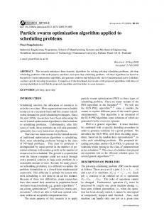
Fig. 3. Benchmark problems examples with clients’ requests having spatially uniform location and symmetric volume distributions (c75), spatially clustered location and skewed volume distributions (c100b), spatially semiclustered location and largely skewed volume distributions (tai100d), and spatially clustered location and largely skewed volume distributions (f71)

number of runs on benchmark problem’s instances. The other parameters were left at their suggested values (from the literature).

6

Discussion and Conclusions

The DVRP discussed in this paper is an important problem not only because of its real world applications but also a possibility to study continuous optimization algorithms in solving dynamic combinatorial tasks. The proposed algorithm achieved better results than other PSO approaches in 6 out of 21 test problems. On Christofides benchmark set, 2-phase PSO best solution was averaged out at 0.96 times the length of the MAPSO and DAPSO best results. On Fisher and Taillard benchmark sets it was 0.99 and 1.06, respectively. The overall result was on average 1.02 times longer in comparison with the best results from 2-phase PSO and other approaches and 1.09 times longer in terms of the average results. Closer analysis of the clients’ requests locations and volume distributions reveals that the proposed algorithm performs better for more spatially clustered benchmarks (e.g. c100b) and for more symmetric volume distributions (e.g. c75). The algorithm’s worst performance on the f71 benchmark set, may be related to the configuration of the largest and the second-largest request in this instance of a DVRP. Those two requests are in a close distance to each other and the joint volume of those requests slightly exceeds the capacity of a vehicle, making the BPP part of the task hard to solve efficiently. Moreover the largest request is

a strong outlier in terms of the request volume. It is more then twice the size of the second-largest request in this particular set. In all other test sets this ratio never exceeds 1.37. The examples of the clients’ requests location and volume distributions are presented in Fig. 3. Overall, the results suggest that the DVRP may be efficiently solved by the PSO even without its hybridization with 2-Opt algorithm. Further research of the proposed algorithm will include the use of alternative encodings of the clients’ assignments, further analysis of the impact of locations and requests distribution on the algorithm’s performance, and application of a multi-swarm approach. Acknowledgements. Study was supported by research fellowship within ”Information technologies: Research and their interdisciplinary applications” agreement number POKL.04.01.01-00-051/10-00. The analysis of the requests distribution within the tests sets has been done with the usage of R[14].

References 1. Standard PSO 2011 (2012), http://www.particleswarm.info/ 2. Vrp web (2012), http://neo.lcc.uma.es/radi-aeb/WebVRP/ 3. Bellaachia, A., Bari, A.: A flocking based data mining algorithm for detecting outliers in cancer gene expression microarray data. In: Information Retrieval Knowledge Management (CAMP), 2012 International Conference on. pp. 305 –311 (march 2012) 4. Blackwell, T.: Particle swarm optimization in dynamic environments. Evolutionary Computation in Dynamic and Uncertain Environments 51, 29 – 49 (2007) 5. Cristian, I., Trelea: The particle swarm optimization algorithm: convergence analysis and parameter selection. Information Processing Letters 85(6), 317 – 325 (2003) 6. Cui, X., Potok, T., Palathingal, P.: Document clustering using particle swarm optimization. In: Swarm Intelligence Symposium, 2005. SIS 2005. Proceedings 2005 IEEE. pp. 185 – 191 (june 2005) 7. Hanshar, F.T., Ombuki-Berman, B.M.: Dynamic vehicle routing using genetic algorithms. Applied Intelligence 27(1), 89–99 (Aug 2007), http://dx.doi.org/10. 1007/s10489-006-0033-z 8. Kennedy, J., Eberhart, R.: Particle swarm optimization. Proceedings of IEEE International Conference on Neural Networks. IV pp. 1942–1948 (1995) 9. Khouadjia, M., Alba, E., Jourdan, L., Talbi, E.G.: Multi-swarm optimization for dynamic combinatorial problems: A case study on dynamic vehicle routing problem. In: Swarm Intelligence, Lecture Notes in Computer Science, vol. 6234, pp. 227–238. Springer, Berlin / Heidelberg (2010), http://dx.doi.org/10.1007/ 978-3-642-15461-4_20 10. Khouadjia, M.R., Sarasola, B., Alba, E., Jourdan, L., Talbi, E.G.: A comparative study between dynamic adapted pso and vns for the vehicle routing problem with dynamic requests. Applied Soft Computing 12(4), 1426 – 1439 (2012), http:// www.sciencedirect.com/science/article/pii/S1568494611004339 11. Kilby, P., Prosser, P., Shaw, P.: Dynamic vrps: A study of scenarios (1998), http: //www.cs.strath.ac.uk/~apes/apereports.html

12. Monson, C.K., Seppi, K.D.: Exposing origin-seeking bias in pso. In: Proceedings of the 2005 conference on Genetic and evolutionary computation. pp. 241–248. GECCO ’05, ACM, New York, NY, USA (2005), http://doi.acm.org/10.1145/ 1068009.1068045 13. Pankratz, G., Krypczyk, V.: Benchmark data sets for dynamic vehicle routing problems (2009), http://www.fernuni-hagen.de/WINF/inhalte/benchmark_data.htm 14. R Core Team: R: A Language and Environment for Statistical Computing. R Foundation for Statistical Computing, Vienna, Austria (2012), http://www.R-project. org/, ISBN 3-900051-07-0 15. R. Montemanni, L. Gambardella, A.R.A.D.: A new algorithm for a dynamic vehicle routing problem based on ant colony system. Journal of Combinatorial Optimization 16. Reynolds, C.W.: Flocks, herds and schools: A distributed behavioral model. SIGGRAPH Comput. Graph. 21(4), 25–34 (Aug 1987), http://doi.acm.org/10. 1145/37402.37406 17. Shi, Y., Eberhart, R.: A modified particle swarm optimizer. Proceedings of IEEE International Conference on Evolutionary Computation p. 69 73 (1998) 18. Shi, Y., Eberhart, R.: Parameter selection in particle swarm optimization. Proceedings of Evolutionary Programming VII (EP98) p. 591 600 (1998) 19. Spears, W. M., G.D.T..S.D.F.: Biases in particle swarm optimization. International Journal of Swarm Intelligence Research 1(2), 34–57 (2010)