Application of Permutation Entropy in Feature Extraction for Near ...

Hindawi Journal of Spectroscopy Volume 2017, Article ID 9165247, 11 pages https://doi.org/10.1155/2017/9165247

Research Article Application of Permutation Entropy in Feature Extraction for Near-Infrared Spectroscopy Noninvasive Blood Glucose Detection Xiaoli Li and Chengwei Li School of Electrical Engineering and Automation, Harbin Institute of Technology, Harbin 150001, China Correspondence should be addressed to Chengwei Li; [email protected] Received 28 December 2016; Revised 20 March 2017; Accepted 16 April 2017; Published 9 August 2017 Academic Editor: Feride Severcan Copyright © 2017 Xiaoli Li and Chengwei Li. This is an open access article distributed under the Creative Commons Attribution License, which permits unrestricted use, distribution, and reproduction in any medium, provided the original work is properly cited. Diabetes has been one of the four major diseases threatening human life. Accurate blood glucose detection became an important part in controlling the state of diabetes patients. Excellent linear correlation existed between blood glucose concentration and near-infrared spectral absorption. A new feature extraction method based on permutation entropy is proposed to solve the noise and information redundancy in near-infrared spectral noninvasive blood glucose measurement, which affects the accuracy of the calibration model. With the near-infrared spectral data of glucose solution as the research object, the concepts of approximate entropy, sample entropy, fuzzy entropy, and permutation entropy are introduced. The spectra are then segmented, and the characteristic wave bands with abundant glucose information are selected in terms of permutation entropy, fractal dimension, and mutual information. Finally, the support vector regression and partial least square regression are used to establish the mathematical model between the characteristic spectral data and glucose concentration, and the results are compared with conventional feature extraction methods. Results show that the proposed new method can extract useful information from near-infrared spectra, effectively solve the problem of characteristic wave band extraction, and improve the analytical accuracy of spectral and model stability.

1. Introduction Diabetes is one of the major diseases threatening human health, and the number of people with diabetes is growing at an alarming rate. More than one hundred million people suffer from diabetes; furthermore, the number is expected to increase to 592 million by 2035 [1]. Although proper diet and insulin injection can be used to regulate blood glucose levels, serious complications are caused in the later stage of diabetes, such as heart failure and blindness [2]. Therefore, the treatment of diabetes is very important, and the concentration of blood glucose detection is the foundation of diabetes treatment. The noninvasive blood glucose detection

technology that measures the glucose concentration in the blood under the condition of no skin damage includes near-infrared spectroscopy, photo acoustic spectroscopy, polarization method, fluorescence method, and dielectric spectroscopy method [3–5]. Compared with the nearinfrared spectra method, other noninvasive blood glucose detection methods are not perfectly suitable for real-time detection. The signals are hard to be detected and easy to be interfered by other components. At present, noninvasive blood glucose detection based on near-infrared spectra has become the research focus at home and abroad. Near-infrared spectroscopy (NIR), which is generated from molecular vibrations and reflects the chemical bond

2 information, such as C-H, O-H, N-H, and S-H, can measure most kinds of compounds and their mixtures. Compared with the traditional analytical techniques, NIR has been widely applied because it is highly efficient and causes no damage and pollution [6–8]. The main structure and composition of glucose information is contained in the near-infrared spectra. The useful glucose information can be extracted form spectral data; then, the data after pretreatment are used to establish a mathematical model to calculate the glucose concentration. In the field of biomedicine, NIR combined with chemometrics is considered one of the most effective methods for noninvasive blood glucose concentration detection [3]. The common chemometrics methods include multiple linear regression (MLR), principal component regression (PCR), partial least squares regression (PLSR), and support vector regression (SVR). The MLR is limited by the noise in spectral data, and the irrelevance between some principal components and the actual content appears in the PCR. Therefore, the PLSR method and SVR method are applied in this paper. However, certain technical difficulties exist in noninvasive blood glucose measurement because near-infrared spectral samples cannot be pretreated, namely, the complex background, overlapped spectral peaks, and less effective information rate. Therefore, extracting effective information from the original spectra is critical for establishing an ideal mathematical model. The effective extraction of glucose characteristic information from nonlinear and nonstationary near-infrared spectral signals can improve the detection efficiency and detection precision. In 1984, Shannon introduced entropy to the field of information theory and proposed the concept of information entropy to measure the uncertainty of events [9]. Subsequently, the concept of entropy was gradually generalized. In 1991, Pincus proposed the concept of approximate entropy (ApEn), which has the advantages of short required calculating data and excellent antinoise ability [10] and offsets the shortcomings of nonlinear analysis. However, the data has no relevance and the errors are produced in the computational process of ApEn. To observably improve the accuracy and efficiency of the ApEn method, Richman and Moorman proposed an improved ApEn in 2000 called sample entropy (SampleEn) [11]. Compared with the ApEn algorithm, SampleEn has short required data and robust antinoise and anti-interference abilities, well consistent in the range of large parameters such unique advantages. The definition of SampleEn must contain a template match; otherwise, it is meaningless. Therefore, Chen et al. improved SampleEn and first defined a new measure of sequence complexity, named fuzzy entropy [12]. This new measure fuzzifies the similarity measure formula with an exponential function to enable the fuzzy entropy value to transition smoothly with changing parameter. Its definition still has significance when the parameter is small, and it inherits the relative consistency and short data setprocessing characteristics of SampleEn. Bandt and Pompe proposed a randomness detection method of a time series, namely, permutation entropy (PE), which can detect the

Journal of Spectroscopy randomness of time series and dynamic mutation behavior [13–18]. Permutation entropy calculates entropy based on permutation patterns by comparing the neighboring values of the time series [19]. PE between 0 and 1 has the advantages of simple concept, fast calculation speed, and robust anti-interference ability, and it is especially suitable for nonlinear data. The key point of near-infrared spectra noninvasive blood glucose detection is to extract the characteristic information from the spectral signal. The near-infrared spectral signals of glucose solution are nonstationary and noisy, but the calculation of PE has a certain antinoise and anti-interference ability. In this study, the feature extraction of spectral information is investigated with glucose solution as the research object from the perspective of whole information from a signal. This paper is organized as follows. Section 2 describes the principles of ApEn, SampleEn, fuzzy entropy, and PE and then briefly introduces the methods of near-infrared spectral characteristic band extraction of a glucose solution, such as fractal dimension, mutual information, and the modeling methods, such as PLSR and SVR. In Section 3, the application of the proposed method is presented, and PLSR and SVR are used to establish calibration models with the extracted characteristic bands, as well as verify the validity and superiority of the proposed method. Finally, the conclusion is drawn in Section 4.

2. Theory and Methods 2.1. Entropy 2.1.1. Approximate Entropy. In 1991, Pincus defined ApEn as a conditional probability that the similarity vector maintains its similarity when it increases from m dimension to m + 1 dimension. The physical meaning is the probability of generating a new pattern of time series when the dimension changes. ApEn has the following advantages: (1) short required data, (2) robust antinoise and anti-interference abilities, and (3) applicability for deterministic and stochastic signals and a mixed signal composed of deterministic and stochastic signals. The steps of the ApEn algorithm are as follows [10]: (1) Given a time series of length N, u i , i = 1, …, N , reconstruct a m-dimensional vector X i , i = 1, 2, …, n, n = N − m + 1, according to the formula X i = u i , u i + 1 , …, u i + m − 1 . (2) Compute the distance between arbitrary the vector X i and the vector X j j = 1, 2, …, N − m + 1, j ≠ i . d ij = max u i + j − u j + k , k = 0, 1, …, m − 1

1

The distance between the two vectors is the maximum absolute value of the difference between two corresponding elements in two vectors.

Journal of Spectroscopy

3

(3) Specify the threshold r, which is typically between 0.2 and 0.3. For each vector X i , find the number of d ij ≤ r × SD (SD is the standard deviation of the sequence) and calculate the ratio between this number and the total number of distances N − m , which is denoted as C m i i . (4) Take the logarithm of C m i i , average for all i, and denote ϕm r . N−m+1 1 〠 ln Cm ϕm r = i r N − m + 1 i=1

(6) Obtain the ApEn from ϕm+1 , ϕm . ApEn = 〠 ϕ − ϕ

m+1

N→∞

−1

N

⋅ 〠 Bm i

(4) Increase the dimension to m + 1 and repeat the above steps to obtain

Bm+1 r = N − m

−1

N

⋅ 〠 Bm+1 i

(5) Theoretically, the SamEn of this sequence is as follows: Bm+1 r Bm r

,

9

3 where N→∞. In practice, N is not an infinite value. When N is a finite value, SamEn is calculated as follows: SampleEn m, r, N = −ln

The parameters N, m, and r in the above steps are the length of time series, length of the comparison window, and margin of similarity, respectively. The bigger the value of m is, the more dynamic the process can be reconstructed. 2.1.2. Sample Entropy. The physical meaning of SampleEn is the same as that of ApEn. The larger SampleEn is, the higher the complexity of the sequence and the greater the probability of generating the new pattern will be. The specific algorithm implementation process is as follows [11]: (1) Given the time series x 1 , x 2 , …, x N , compose a set of dimension vectors according to the serial number order.

Bm+1 r Bm r

10

2.1.3. Fuzzy Entropy. In the definition of fuzzy entropy, the concept of a fuzzy set is introduced, and the exponential function is chosen as the fuzzy function to measure the similarity of two vectors. The exponential function has the following expectation properties: (1) continuity of the exponential function ensures that its value does not have a mutation and (2) the nature of the exponential function ensures that the self-similarity value of the vector is maximum. The definition of fuzzy entropy is as follows [12]: (1) The sampling sequence u i : 1≪i≪N .

with

N

points

is

(2) Compose a set of m-dimensional vectors according to the serial number order.

X m i = x i , x i + 1 , …, x i + m − 1 ,   5

Xm i = u i , u i + 1 , …, u i + m − 1

(2) Define the distance between vector X m i and vector X m j as the largest difference between their corresponding elements, namely, d X m i , X m j = max x i + k − x j + k

8

i=1

SampleEn m, r = limN→∞ −ln

(7) For a finite time series, ApEn can be estimated by a statistical value. 4 ApEn = ϕm − ϕm+1

i=1 N−m

7

i=1

2

(5) Increase m by 1 and repeat steps 1 to 4 to obtain C m+1 i and ϕm+1 r . i

m

Bm r = N − m

6

(3) Define the threshold r. For the value of each i ≤ N − m, find the number N i of d X m i , X m j ≤ r, and calculate the ratio between N i and the total number of distances N − m − 1, which is denoted as Bm i = N i / N − m − 1 . The average for all i is as follows:

− u0 i

i = 1, …, N − m ,

11

where u i , u i + 1 , …, u i + m − 1 represents the continuous m values of u starting from the ith point. u0 i is its mean value. u0 i =

1 m−1 〠 u i+j m j=0

12

m (3) Define the distance d m ij between vector X i and vector m X j as the largest difference between their corresponding elements, namely,

4

Journal of Spectroscopy where m and τ are the embedding dimension and delay time, respectively, and K = n − m − 1 τ. Each row in the matrix = maxk∈ 0,m−1 u i + k − u0 i − u j + k − u0 j ,   can be regarded as a reconstructed component, with a total of K reconstruction components. The jth reconstruction i, j = 1 N − m, j ≠ i component x j , x j + τ , …, x j + m − 1 τ of the reconstruction matrix X i is rearranged according to the values 13 in ascending order. j1 , j2 , …, jm represents the index of the m (4) Define the similarity Dm column in which the individual elements of the reconstructed ij between vector X i and m vector X m component are as follows: j , with a fuzzy function d ij , n, r , namely, m m dm ij = d X i , X j

Dm ij =

dm ij , n, r = exp

− dm ij

n

r

,

14

where the fuzzy function d m ij , n, r is an exponential function, and n and r are the gradient and width of the exponential function boundary, respectively. (5) Define the function as follows: Om n, r =

N−m 1 N−m 1 〠 〠 Dm N − m i=1 N − m − 1 j=1,j≠i ij

15

(6) Similarly, repeat steps 2 to 5, reconstruct a set of m + 1-dimensional vector according to the serial number order, and define the following function: Om n, r =

N−m 1 N−m 1 〠 〠 Dm+1 N − m i=1 N − m − 1 j=1,j≠1 ij

16 (7) Define the fuzzy entropy as follows: FuzzyEn m, n, r = limN→∞ ln Om n, r − ln Om+1 n, r

17

When N is a finite value, the value obtained by the above steps is the estimated value of the fuzzy entropy of the sequence with length N.

x i + j1 − 1 τ ≤ x i + j 2 − 1 τ ≤ ⋯ ≤ x i + j m − 1 τ

20

If equal values in the reconstructed component are observed, x i − j1 − 1 τ = x i − j m − 1 τ ,

21

the components are arranged according to the size of the value of j1 and j2 , that is, when j1 < j2 , x i − j1 − 1 τ ≪ x i − j2 − 1 τ . Therefore, for an arbitrary time series X i , a set of symbol sequences can be obtained from each row in the reconstructed matrix S l = j1 , j2 , …, jm ,

22

where l = 1, 2, …, k and k ≪ m . m is observed when the m-dimensional phase space map has a different symbolic sequence j1 , j2 , …, jm , and the symbolic sequence S l is one kind of arrangement. If the probability of the occurrence of each symbol sequence is P1 , P2 , …, Pk , the PE of k kinds of different symbol sequences of time series X i in terms of Shannon entropy is as follows: k

H p m = −〠 Pj ln Pj

23

j=1

When Pj = 1/m , H p m reaches the maximum value ln m . For convenience, H p m is typically normalized with ln m , namely,

FuzzyEn m, n, r, N = ln Om n, r − ln Om+1 n, r 18 2.1.4. Permutation Entropy. According to [13], the definition of PE is setting a time sequence X i , i = 1, 2, …, n , and reconstruct it in phase space to obtain the matrix x 1

x 1+τ

⋮

⋮

x j

x j+τ

⋮

⋮

x K

x K +τ

⋯

x 1 + m−1 τ ⋮

⋯

x j + m− 1 τ

,  j = 1, 2, …, K,

⋮ ⋯

x K m− 1 τ 19

0 ≪ Hp =

Hp ln m ≪ 1

24

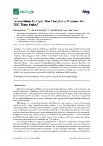
The magnitude of H p represents the randomness degree of the time series X i . The smaller the value of H p is, the more inerratic the time series will be; otherwise, the more stochastic the time series will be. The change in H p reflects and amplifies the minute details of the time series. 2.1.5. Application to Simulation Signal. In order to compare the ApEn, SampleEn, fuzzy entropy, and PE, define a mixed signal composed of deterministic signal and stochastic signal with a different probability, MIX N, p = 1 − p x t + py t ,

25

Journal of Spectroscopy

5

1.2

1

Entropy value

0.8

0.6

0.4

0.2

0

0

1

2

3

4

5

A ApEn1 SampleEn1 FuzzyEn1

PE1 ApEn2 SamleEn2

FuzzyEn2 PE2

Figure 1: Four kinds of entropy values with different amplitudes. 1.2

Entropy value

1 0.8 0.6 0.4 0.2 0 128

256

512

1024

2048 N

ApEn1 SampleEn1 FuzzyEn1

PE1 ApEn2 SampleEn2

FuzzyEn2 FE2

Figure 2: Four kinds of entropy values with different data lengths.

where x t = 2sin 2πt , y t is the stochastic signal in −0 5, 0 5 , N is the data length, and p ∈ 0, 1 . Considering the four kinds of entropy of signal with MIX 1024, 0 4 and MIX 1024, 0 2 , note ApEn1, SampleEn1, FuzzyEn1, PE1, ApEn2, SampleEn2, FuzzyEn2, and PE2 for convenience, respectively. Their change relation with signal amplitude A, signal length N, and signal-to-noise ratio of signal are shown in Figures 1–3. Figure 1 shows that ApEn, SampleEn, and FuzzyEn change slightly with the same probability, when signal amplitude A changes bigger gradually. However, the PE

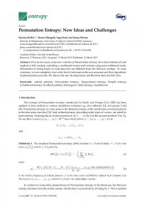
has been the same all the time with a different probability, which illustrates that the PE has excellent stability and consistency. Figure 2 shows that the ApEn, SampleEn, and FuzzyEn change with the signal length N and remain unchanged after N = 512 with the same probability, which illustrates that the values of ApEn, SampleEn, and FuzzyEn are related to the data length. However, the PE has been the same all the time with a different probability, which illustrates that the required time sequence of PE is shorter in the calculation process.

6

Journal of Spectroscopy 2.5

Entropy value

2

1.5

1

0.5

0 −13

−11

−9

−7

−5

−3

−1

1

3

5

7

9

11

13

SNR ApEn1 SampleEn1 FuzzyEn1

PE1 ApEn2 SampleEn2

FuzzyEn2 PE2

Figure 3: Four kinds of entropy values with different signal-to-noise ratios of signal.

Figure 3 shows that the ApEn, SampleEn, and FuzzyEn change with the signal-to-noise ratio of the signal as the same trend with the same probability, which illustrates that the values of ApEn, SampleEn, and FuzzyEn are affected by SNR of the signal. However, the PE has been the same all the time with a different probability, which illustrates that the PE has robust antinoise ability. Therefore, the PE is used for extracting the feature information of near-infrared spectral data of glucose solution in this study. 2.2. Fractal Dimension. Dimension, an important feature of geometry, characterizes the size of the space a shape occupies. Because Euclidean geometry objects are relatively regular shapes, the obtained dimension is an integer. However, Euclidean geometry is not applied for irregular complex shapes. Most natural geometries exhibit similar properties. Therefore, the spatial dimension of an object is not always an integer; it can also be fractional. The noninteger dimension is the real dimension of most geometric shapes; integers are only special cases. The noninteger dimension is a different concept, but it is suitable for all the geometric shapes in nature. In 1919, Hausdorff, who studied the properties of singular sets, first proposed the concept of fractal dimension [20] and defined the Hausdorff measure and dimension theory. Since then, several scholars have developed various dimensions, such as selfsimilar dimension, box dimension, information dimension, correlation dimension, and Lyapunov dimension. The box dimension is one of the most common fractal dimensions because of its ease of calculation, few parameters, and ease of application. The box dimension is defined as the way that the set X is covered by a hypercube with size ε. X is a nonempty and bordered subset Rn . If it is covered by N ε hypercube with length ε, then

DB X = limε→0

ln N ε ln 1/ε

26

The above formula is the definition of the fractal box dimension. The steps are as follows: (1) Set discrete signal y i ⊂ Y, and Y is the closed set in the n-dimensional Euclidean space Rn . (2) Divide Rn with the ε grids as small as possible, and N ε is the grid counts of set Y. The limit in the above formula cannot be determined by definition; so, an approximate method is used in calculation. The ε grid is used as the reference, and it is enlarged to the kε grid, where k ∈ Z + . In this way, N kε N kε is the grid count of set Y in discrete space, and the following formula can be obtained: N/k

P kε = 〠 max yk i−1 +1 , yk i−1 +2 , …, yk i−1 +k+1 i=1

− min yk i−1 +1 , yk i−1 +2 , …, yk i−1 +k+1 ,

27 where i = 1, 2, …, N/k, k = 1, 2, …, M, M < N, and N is the number of sampling points. The grid count is as follows: N kε =

P kε + 1, kε

28

where N kε > 1. In the graph of lgkε − lgN kε , the scalefree region is determined with good linearity. The beginning and end points of the scale-free region are k1 and k2 ; thus,

Journal of Spectroscopy

7

lgN kε = algkε + b, k1 ≤ k ≤ k2

29

Finally, the slope of the line is determined by the least square method, â =

k2 − k1 + 1 〠lgk〠lgN kε − 〠lgk〠lgN kε k2 − k1 + 1 〠lg2 k − 〠lgk

2

30

The box dimension DB is as follows: DB = â

31

2.3. Mutual Information. Information is the movement state and the way the movement state changes items that are felt and expressed by the cognitive subject. Two kinds of metric forms are identified for information. One measures how much information the message or message collection itself contains; another one is the measure of how much information is provided between messages or message sets. The former is described by self-information entropy and message entropy, whereas the latter is described by mutual information (MI) and average mutual information. Mutual information measures the degree of interdependence between two variables and represents the amount of shared information between two variables. For two given random variables X and Y, if their respective marginal probability distribution and joint probability distribution are p x , p y , and p x, y , the definition of mutual information between them is as follows: p x, y I X Y = 〠 〠 p x, y log px py x y

32

When the variables X and Y are completely unrelated or independent with each other, the mutual information is the minimum 0, which means no information overlaps between the two variables. By contrast, the higher the degree of interdependence between the two variables is, the greater the value of mutual information will be, and the more similar the information it contains. 2.4. Partial Least Squares Regression. In 1984, Wold and Albano first proposed PLSR, which was a new multivariate statistical data analysis method and studied the regression modeling of multiple dependent variables [21]. Given p independent variables x1 , x2 , …, xp and q dependent variables, the study of the statistical relationship between the independent variable and dependent variable involves the observation of n sample points, which form the data tables X and Y of the independent variable and dependent variable. In PLSR, the components t 1 and u1 are first extracted form X and Y; namely t 1 is the linear combination of x1 , x2 , …, xp and u1 is the linear combination of y1 , y2 , …, yq . After the first components t 1 and u1

are extracted, the regression of X on t 1 and Y on u1 is performed by PLSR. The accuracy of the model is validated; if the regression equation reaches satisfactory accuracy, the algorithm is terminated. Otherwise, the residual information of X interpreted by t 1 and the residual information of Y interpreted by u1 will be extracted for the second round. This step is repeated until accuracy is satisfactory. Finally, if m components t 1 , t 2 , …, t m form X, PLSR can be expressed as the regression equation of yk about the original variables x1 , x2 , …, xp by implementing regression with yk k = 1, 2, …, q on t 1 , t 2 , …, t m . 2.5. Support Vector Regression. The support vector machine (SVM) is a new machine learning method proposed by Vapnik et al. based on statistical learning theory. SVM has the characteristics of small sample learning and strong generalization ability, which can avoid the problems of overlearning and local minimum. By introducing the insensitive loss function ε, Vapnik et al. have extended the SVM to the regression estimation of the nonlinear system and established the SVR algorithm. SVR has been widely used in function estimation, nonlinear system modeling, and other fields [22]. For the sample set G = xi , yi ni (xi is the input vector, yi is the corresponding target value, and n is the number of samples), the SVR function is as follows: f x = ωϕ x + b,

33

where ϕ x is the nonlinear map transforming data into a high-dimension feature space and ω and b are coefficients. 2.6. Near-Infrared Spectra Data. In the near-infrared spectra noninvasive blood glucose measurement experiments, the blood glucose solution is temporarily replaced by glucose solution. All the glucose solutions, which concentration ranges from 50 mg/dL to 1000 mg/dL, are continuous and are equally distributed liquid that is uniformly configured under the same conditions. The prepared samples of glucose solution are put into the detection system of spectrometer. All the experimental data are collected by Fourier spectrometer Antaris II FT-NIR, produced by America Thermo Company. Its spectral range is 833–2630 nm, resolution is 4 cm−1 across spectral range, wavenumber reproducibility is better than 0.05 cm−1, and wavenumber accuracy is ±0.03 cm−1. The data meet the measurement principle of Lambert-Beer’s law. All the collected near-infrared spectral data of glucose solution are measured five times with the same concentration in order to get a small statistical error and shown in Figure 4.

3. Results and Discussion The principle of selecting optimal wave bands has two key points: (1) information on the selected bands is large and (2) the correlation between bands is small. The widely used extraction methods include the information comparison of each band, information correlation between bands, best

8

Journal of Spectroscopy 8 7

Absorbance

6 5 4 3 2 1

5000

6000

7000

8000

9000

10000

11000

12000

Wavenumber (cm−1) 50 mg/dL 60 mg/dL 70 mg/dL 80 mg/dL 90 mg/dL

100 mg/dL 200 mg/dL 300 mg/dL 400 mg/dL 500 mg/dL

600 mg/dL 700 mg/dL 800 mg/dL 900 mg/dL 1000 mg/dL

Figure 4: Near-infrared spectral data of glucose solution.

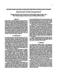
index method, entropy, and joint entropy of band data. In feature extraction, the fractal dimension (FD) can be used as a feature because almost all signals have fractal characteristics. The fractal dimension can distinguish different signals on the premise that two signals have different dimensions under the same measure. If two signals come from the same state, they have similarities, and their fractal dimensions are similar. The correlation or correlation coefficient can only reflect the linear correlation between two variables but cannot measure the nonlinear relationship between them. However, from the view of information theory, mutual information can estimate the total information amount between variables, is not limited to a linear relationship, and has greater advantages than correlation comparison. PE analysis can effectively determine the similarity between sequences and show the strong similarity and distinction, which can be further applied to biological sequence analysis. PE of the time series is calculated using the PE algorithm. The ratio value of PE is the basis for analyzing the similarity between sequences. Therefore, the PE, fractal dimension, and mutual information are used in extracting the feature information of near-infrared spectral data of glucose solution in this study. In the PE calculation, there are three parameters needed to be considered and set, namely, data length N, embedded dimension m, and time delay λ. According to reference [23], λ has a little effect on the PE value and there are very small differences among the PE values with different λ. Therefore, λ = 1 is chosen in this study. In order to discuss the relationship of N and m with PE value, the PE values of the given signal MIX N, p with data length 128, 256, 512, 1024, and 2048 are calculated in Figure 5. Figure 5 shows that the PE values are almost same in m = 2, 3, 4 with different

data length N. If m is too small, the algorithms lose significance and effectiveness because of the few states contained in reconstructed sequence. If m is too big, the time series will be homogenized by phase space reconstruction; thus, the computation is time-consuming and the subtle changes in sequence cannot be reacted. Therefor m = 3 and N = 1867, which is the length of collected spectra data, are chosen in this study. Because PE cannot be affected by noise (λ = 1), the characteristic wave bands are extracted from the collected near-infrared spectroscopy data of the glucose solution. Full spectral wavelength data have 1867 points in total, which are divided into wavelength intervals with 50, 100, 150, and 200 points. The ratio of PE of the corresponding wavelength interval between 50 mg/dL, 500 mg/dL, 1000 mg/dL, and pure water solution, the ratio of FD of the corresponding wavelength interval between 50 mg/dL, 500 mg/dL, 1000 mg/dL, and pure water solution and the MI values of the corresponding wavelength interval between 50 mg/dL, 500 mg/dL, 1000 mg/dL, and pure water solution are shown in Figure 6. As shown in Figure 6, the ratios of FD values and MI values of each wavelength interval have no obvious difference. The PE values of some wavelength intervals are substantially consistent, and other wavelength intervals are significantly different. Therefore, the later wavelength intervals are the characteristic wave bands that contained abundant glucose concentration information. However, the PE values of wavelength intervals that are divided with less than 50 points or more than 200 points of different concentration spectra have no obvious distinguished law. In order to improve the precision and accuracy of feature wavelength extraction, the characteristic wavelength intervals are extracted in four uniform ways (50, 100, 150, and 200), and their overlapping

Journal of Spectroscopy

9

1

PE value

0.8

0.6

0.4

0.2

0

2

3

4

5 m

6

N = 128 N = 256 N = 512

7

8

N = 1024 N = 2048

Figure 5: The PE value of different lengths N and embedded dimensions m of signal.

7

6

6

5

5 Value

Value

4 3 2

3 2

1 0

4

1 1

3

5

7

0

9 11 13 15 17 19 21 23 25 27 29 31 33 35 37 39

1

2

3

4

5

6

7

Segment number FD (50 mg/dL) FD (500 mg/dL) FD (1000 mg/dL)

PE (50 mg/dL) PE (500 mg/dL) PE (1000 mg/dL)

FD (50 mg/dL) FD (500 mg/dL) FD (1000 mg/dL)

MI (50 mg/dL) MI (500 mg/dL) MI (1000 mg/dL)

PE (50 mg/dL) PE (500 mg/dL) PE (1000 mg/dL)

7

7

6

6

5

5

4

4

3

3

2

2

1

1 2

3

4

5

6

7

8

9

10

11

12

13

0

1

2

3

PE (50 mg/dL) PE (500 mg/dL) PE (1000 mg/dL)

(c)

4

5

6

7

8

9

10

Segment number

Segment number FD (50 mg/dL) FD (500 mg/dL) FD (1000 mg/dL)

MI (50 mg/dL) MI (500 mg/dL) MI (1000 mg/dL)

(b) 8

Value

Value

(a)

1

9 10 11 12 13 14 15 16 17 18 19

Segment number

8

0

8

MI (50 mg/dL) MI (500 mg/dL) MI (1000 mg/dL)

FD (50 mg/dL) FD (500 mg/dL) FD (1000 mg/dL)

PE (50 mg/dL) PE (500 mg/dL) PE (1000 mg/dL)

MI (50 mg/dL) MI (500 mg/dL) MI (1000 mg/dL)

(d)

Figure 6: PE, FD, and MI of segmented spectral data: (a) 50 mg/dL, (b) 100 mg/dL, (c) 150 mg/dL, and (d) 200 mg/dL.

10

Journal of Spectroscopy Table 1: Extraction of feature wave bands by PE.

Number 1 2 3 4

Segment number 7, 8, 17, 19 4, 9, 14 3, 5 4

Overlapping wavenumber (cm−1)

6840–7230, 8680–8880

Table 2: R and RMSEP of SVR model. Method PE EMD-SPA SPA FD MI Full spectra data

R 0.9998 0.9892 0.9542 0.9293 0.8990 0.8188

RMSEC (%) 0.0346 0.0670 0.0846 0.1050 0.1522 0.2499

Table 3: R and RMSEP of PLSR model. Method PE EMD-SPA SPA FD MI Full spectra data

R 0.9897 0.9688 0.9321 0.9089 0.8880 0.8076

RMSEC (%) 0.0468 0.0822 0.1045 0.1276 0.1601 0.2519

intervals are considered as the final characteristic wavelength intervals (Table 1). In order to verify the effectiveness of the proposed method, the characteristic wavelength intervals of the collected spectral data of glucose solutions with the FD method, MI method, the proposed method, successive projection algorithm (SPA) method [24], EMD-SPA method [25], and full spectral data are taken into the calibration models that were established by PLSR and SVR. The correlation coefficient and root mean square error correction (RMSEC) of the model are evaluated. The characteristic wavelength points that were extracted based on the PE method are 150, which is much less than the full spectral wavelength points, and the smaller selected characteristic wavelength points are, the shorter the established model time is. The experimental results of SVR and PLSR calibration model (Tables 2 and 3) show that the correlation coefficient (R) and RMSEC of established calibration model by characteristic wavelength intervals that were extracted based on the PE method reach 0.9998/0.9897 and 0.0346%/0.0468%. The results are better than that of the established calibration model by characteristic wavelength intervals that were extracted based on FD method, MI method, SPA method, EMD-SPA method, and by full spectra data. The overall modeling results of SVR are more reliable to that of PLSR modeling method.

4. Conclusions The feature wave band extraction method that was based on permutation entropy that is proposed in this study for near-infrared spectra noninvasive blood glucose detection. The spectra data do not need denoise because PE has the advantages of robust antinoise and anti-interference abilities, and it is especially suitable for nonlinear data. Taking the near-infrared spectra data of glucose solutions as the object, all of the collected near-infrared spectra are divided with different interval points, and the ratio values of PE of corresponding spectra intervals are calculated. The overlap spectral intervals contained abundant glucose concentration information, which were extracted for reducing the effective range of data. Then, the PLSR and SVR methods are introduced for establishing the calibration models with characteristic spectra that were extracted by the proposed method, FD method, MI method, SPA method, EMD-SPA method, and full spectral data. According to the correlation coefficient and RMSEC of the calibration models, the proposed feature extraction method effectively solves the redundancy problem of near-infrared spectra data, and it also improves the robustness and predictive ability of regression model.

Conflicts of Interest The authors declare that there is no conflict of interests regarding the publication of this paper.

Acknowledgments This work was supported by the Program for Harbin City Science and Technology Innovation Talents of Special Fund Project (Grant no. 2014RFXXJ065) and the Fundamental Research Funds for the Central Universities (Grant no. HIT. IBRSEM. 201307).

References [1] L. Guariguata, D. R. Whiting, I. Hambleton, J. Beagley, U. Linnenkamp, and J. E. Shaw, “Global estimates of diabetes prevalence for 2013 and projections for 2035,” Diabetes Research and Clinical Practice, vol. 103, no. 2, pp. 137– 149, 2014. [2] D. Ding, Near Infrared Spectroscopy Research and Application in Biomedicine, Ph.D. thesis, JiLin University, 2004. [3] C. E. Ferrante do Amaral and B. Wolf, “Current development in non-invasive glucose monitoring,” Medical Engineering & Physics, vol. 30, no. 5, pp. 541–549, 2008. [4] A. Duncan, J. Hannigan, S. S. Freeborn et al., “A portable non-invasive blood glucose monitor,” in The International Conference on Solid-State Sensors and Actuators, pp. 455– 458, Stockholm, Sweden, June 1995. [5] J. R. Blanco, F. J. Ferrero, J. C. Campo et al., “Design of a low-cost portable potentiostat for amperometric biosensors,” in IEEE Instrumentation & Measurement Technology Conference, pp. 690–694, Sorrento, April 2006. [6] J. Y. Tang, M. H. Wang, M. K. Chen, and L. S. Jang, “Glucose detection using an electro-optical fluidic device

Journal of Spectroscopy

[7]

[8]

[9]

[10]

[11]

[12]

[13]

[14]

[15]

[16]

[17]

[18]

[19]

[20]

[21]

based on pulse width modulation,” in Seventh International Conference on Sensing Technology, pp. 325–329, Wellington, December 2013. S. Ramasahayam, K. S. Haindavi, B. Kavala, and S. R. Chowdhury, “Noninvasive estimation of blood glucose using near infrared spectroscopy and double regression analysis,” in Seventh International Conference on Sensing Technology, pp. 627–631, Wellington, December 2013. K. A. Unnikrishna Menon, D. Hemachandran, and T. K. Abhishek, “A survey on non-invasive blood glucose monitoring using NIR,” in International Conference on Communications and Signal Processing (ICCSP), pp. 1069–1072, Melmaruvathur, April 2013. C. E. Shannon, “A mathematical theory of communication,” Bell System Technical Journal, vol. 27, no. 3, pp. 379–423, 1948. S. M. Pincus, “Approximate entropy as a measure of system complexity,” Proceedings of the National Academy of Sciences of the United States of America, vol. 88, no. 6, pp. 2297–2301, 1991. J. S. Richman and J. R. Moorman, “Physiological time-series analysis using approximate entropy and sample entropy,” American Journal of Physiology Heart and Circulatory Physiology, vol. 278, no. 6, pp. H2039–H2049, 2000. W. Chen, Z. Wang, H. Xie, and W. Yu, “Characterization of surface EMG signal based on fuzzy entropy,” IEEE Transactions on Neural Systems and Rehabilitation Engineering, vol. 15, no. 2, pp. 266–272, 2007. C. Bandt and B. Pompe, “Permutation entropy: a natural complexity measure for time series,” Physical Review Letters, vol. 88, no. 17, article 174102, 2002. L. Zunino, M. C. Soriano, I. Fischer, O. A. Rosso, and C. R. Mirasso, “Permutation-information-theory approach to unveil delay dynamics from time-series analysis,” Physical Review E, Statistical, Nonlinear, and Soft Matter Physics, vol. 82, no. 4, Part 2, pp. 565–590, 2010. X. Li, D. Ph, S. Cui, and L. J. Voss, “Using permutation entropy to measure the electroencephalographic effects of sevoflurane,” Anesthesiology, vol. 109, no. 3, pp. 448–456, 2008. Y. Liu, T.-S. Chon, H. Baek, Y. Do, J. H. Choi, and Y. D. Chung, “Permutation entropy applied to movement behaviors of Drosophila melanogaster,” Modern Physics Letters B, vol. 25, no. 12n13, pp. 1133–1142, 2011. M. Zanin, L. Zunino, O. A. Rosso, and D. Papo, “Permutation entropy and its main biomedical and econophysics applications: a review,” Entropy, vol. 14, no. 8, pp. 1553–1577, 2012. C. Bian, C. Qin, Q. D. Y. Ma, and Q. Shen, “Modified permutation-entropy analysis of heartbeat dynamics,” Physical Review E, Statistical, Nonlinear, and Soft Matter Physics, vol. 85, no. 2, Part 1, article 021906, 2012. Z. Shi, W. Song, and S. Taheri, “Improved LMD, permutation entropy and optimized K-means to fault diagnosis for roller bearings,” Entropy, vol. 18, no. 3, p. 70, 2016. A. Accardo, M. Affinito, M. Carrozzi, and F. Bouquet, “Use of the fractal dimension for the analysis of electroencephalographic time series,” Biological Cybernetics, vol. 77, no. 5, pp. 339–350, 1997. S. Wold, C. Albano, W. J. Dunn et al., “Modelling data tables by principal components and PLS: class patterns and quantitative predictive relations,” Analusis, vol. 12, no. 10, pp. 477–485, 1984.

11 [22] A. J. Smola and B. Schölkopf, “A tutorial on support vector regression,” Statistics and Computing, vol. 14, no. 3, pp. 199–222, 2002. [23] J. Zheng, J. Cheng, and Y. Yang, “Multiscale permutation entropy based rolling bearing fault diagnosis,” Shock and Vibration, vol. 1, pp. 1–8, 2014. [24] G. Y. Hui, L. J. Sun, J. N. Wang, L. K. Wang, and C. J. Dai, “Research on the pre-processing methods of wheat hardness prediction model based on visible-near infrared spectroscopy,” Spectroscopy and Spectral Analysis, vol. 36, pp. 2111– 2116, 2012. [25] Z. Y. Zhang, G. Li, L. Lin, and B. J. Zhang, “Application of EMD and SPA algorithm in the detection of benzoyl peroxide addition in flour by spectroscopy,” Spectroscopy and Spectral Analysis, vol. 32, no. 10, pp. 2815–2819, 2012.

International Journal of

Medicinal Chemistry Hindawi Publishing Corporation http://www.hindawi.com

Volume 2014

Photoenergy International Journal of

Organic Chemistry International Hindawi Publishing Corporation http://www.hindawi.com

Volume 2014

Hindawi Publishing Corporation http://www.hindawi.com

Volume 201

International Journal of

Analytical Chemistry Hindawi Publishing Corporation http://www.hindawi.com

Volume 2014

Advances in

Physical Chemistry Hindawi Publishing Corporation http://www.hindawi.com

Volume 2014

International Journal of

Carbohydrate Chemistry Hindawi Publishing Corporation http://www.hindawi.com

Journal of

Quantum Chemistry Hindawi Publishing Corporation http://www.hindawi.com

Volume 2014

Volume 2014

Submit your manuscripts at https://www.hindawi.com Journal of

The Scientific World Journal Hindawi Publishing Corporation http://www.hindawi.com

Journal of

International Journal of

Inorganic Chemistry Volume 2014

Journal of

Theoretical Chemistry

Hindawi Publishing Corporation http://www.hindawi.com

Hindawi Publishing Corporation http://www.hindawi.com

Volume 2014

Spectroscopy Hindawi Publishing Corporation http://www.hindawi.com

Analytical Methods in Chemistry

Volume 2014

Hindawi Publishing Corporation http://www.hindawi.com

Volume 2014

Chromatography Research International Hindawi Publishing Corporation http://www.hindawi.com

Volume 2014

International Journal of

Electrochemistry Hindawi Publishing Corporation http://www.hindawi.com

Volume 2014

Journal of

Hindawi Publishing Corporation http://www.hindawi.com

Volume 2014

Journal of

Catalysts Hindawi Publishing Corporation http://www.hindawi.com

Journal of

Applied Chemistry

Hindawi Publishing Corporation http://www.hindawi.com

Bioinorganic Chemistry and Applications Hindawi Publishing Corporation http://www.hindawi.com

Volume 2014

International Journal of

Chemistry Volume 2014

Volume 2014

Spectroscopy Volume 2014

Hindawi Publishing Corporation http://www.hindawi.com

Volume 2014